Connecting curves for dynamical systems

Abstract

We introduce one dimensional sets to help describe and constrain the integral curves of an $n$ dimensional dynamical system. These curves provide more information about the system than the zero-dimensional sets (fixed points) do. In fact, these curves pass through the fixed points. Connecting curves are introduced using two different but equivalent definitions, one from dynamical systems theory, the other from differential geometry. We describe how to compute these curves and illustrate their properties by showing the connecting curves for a number of dynamical systems.

Keywords: Differential Geometry; curvature; torsion; chaotic dynamical systems

I Introduction

Poincaré proposed that the fixed points of a dynamical system could be used to provide some information about, or constraints on, the behavior of trajectories defined by a set of $n$ nonlinear ordinary differential equations (a dynamical system) Poin81 ; Poin82 ; Poin85 ; Poin86 . The fixed points of a dynamical system constitute its zero-dimensional invariant set. Unfortunately, the fixed points provide only local information about the nature of the flow.

Since that time many, including Andronov, Tikhonov, Levinson, Wasow, Cole, O’Malley and Fenichel, have focused on higher dimensional invariant sets, in particular on $n-1$ dimensional invariant sets. In many instances these are slow invariant manifolds of singularly perturbed dynamical systems. These manifolds enable one to define the slow part of the evolution of the trajectory curve of such systems. Until now, it seems that, except for the works of Roth98 , no one has investigated the problem of one-dimensional sets which play a very important role in the structure of chaotic attractors by connecting their fixed points. The aim of this work is to define and present methods for constructing such one-dimensional sets. The sets that we construct are generally not trajectories that satisfy the equations of the dynamical system.

The first attempt to study one-dimensional sets has been made in the context of Fluid Mechanics by Roth and Peikert Roth98 . The idea of transporting the concept of “vortex core curves” to the phase space of dynamical systems is due to one of us (R.G.), who applied it to three-dimensional dynamical systems and then to higher-dimensional dynamical systems. In the context of classical differential geometry, another of us (J.M.G.) called such curves connecting curves since they are one-dimensional sets that connect fixed points.

In Sec. II we set terminology by introducing autonomous dynamical systems and define the velocity and acceleration vector fields in terms of the forcing equations for these systems. In Sec. III we introduce the idea of the vortex core curve through an eigenvalue-like equation derived from the condition that one of the eigendirections of the Jacobian of the velocity vector field is colinear with the velocity vector field. We show that this defines a one-dimensional curve in the phase space. In Sec. IV we introduce the idea of connecting curves from the viewpoint of differential geometry. These are defined by the locus of points where the curvature along a trajectory vanishes. In Sec. V we show that the two definitions are equivalent. In Sec. VI we describe three methods for computing the connecting curves for a dynamical system. Several applications are described in Sec. VII including two models introduced by Rössler, two introduced by Lorenz, and a dynamical system with a high symmetry. The figures show clearly that the connecting curve plays an important role as an axis around which the flow rotates, which is why this curve is called the vortex core curve in hydrodynamics. The figures also underline an observation made in Roth98 that this curve is at best an approximation to the curve around which the flow swirls. In the final Section we summarize our results and provide a pointer to visual representations of many other dynamical systems and their connecting curves.

II Dynamical systems

We consider a system of differential equations defined in a compact $E$ included in $\mathbb{R}^{n}$ with $\vec{X}=\left[{x_{1},x_{2},...,x_{n}}\right]^{t}\in E\subset\mathbb{R}^{n}$:

$$\frac{d\vec{X}}{dt}=\overrightarrow{\Im}(\vec{X})$$ (1)

where $\overrightarrow{\Im}(\vec{X})=\left[f_{1}(\vec{X}),f_{2}(\vec{X}),...,f_{n}(\vec{X})\right]^{t}\subset\mathbb{R}^{n}$ defines a velocity vector field in $E$ whose components $f_{i}$ are assumed to be continuous and infinitely differentiable with respect to all $x_{i}$, i.e., are real-valued $C^{\infty}$ functions (or $C^{r}$ for $r$ sufficiently large) in $E$ and which satisfy the assumptions of the Cauchy-Lipschitz theorem Codd55 . A solution of this system is the parameterized trajectory curve or integral curve $\vec{X}\left(t\right)$ whose values define the states of the dynamical system described by Eq. (1). Since none of the components $f_{i}$ of the velocity vector field depends here explicitly on time, the system is said to be autonomous.

As the vector function $\vec{X}\left(t\right)$ of the scalar variable $t$ represents the trajectory of a particle M, the total derivative of $\vec{X}\left(t\right)$ is the vector function $\overrightarrow{V}\left(t\right)$ of the scalar variable $t$ which represents the instantaneous velocity vector of M at the instant $t$, namely:

$$\overrightarrow{V}\left(t\right)=\frac{d\vec{X}}{dt}=\overrightarrow{\Im}(\vec{X})$$ (2)

The instantaneous velocity vector $\overrightarrow{V}\left(t\right)$ is tangent to the trajectory except at the fixed points, where it is zero.

The time derivative of $\overrightarrow{V}\left(t\right)$ is the vector function $\vec{\gamma}\left(t\right)$ that represents the instantaneous acceleration vector of M at the instant $t$

$$\vec{\gamma}\left(t\right)=\frac{d\overrightarrow{V}}{dt}$$ (3)

Since the functions $f_{i}$ are supposed to be sufficiently differentiable, the chain rule leads to the derivative in the sense of Fréchet Frec25 :

$$\frac{d\overrightarrow{V}}{dt}=\frac{\partial\overrightarrow{\Im}}{\partial\vec{X}}\frac{d\vec{X}}{dt}$$ (4)

By noticing that $\frac{\partial\overrightarrow{\Im}}{\partial\vec{X}}$ is the functional Jacobian matrix $J$ of the dynamical system (1), it follows from Eqs. (3) and (4) that

$$\vec{\gamma}=J\overrightarrow{V}$$ (5)

This equation plays a very important role in the discussions below.

III Dynamical Systems and Vortex Core Curves

At a fixed point in phase space the eigenvectors of the Jacobian matrix define the local stable and unstable manifolds. At a general point in phase space the eigenvectors of the Jacobian with real eigenvalues define natural displacement directions. There may be points in the phase space where two eigenvalues form a complex conjugate pair and one is real, and the real eigenvector is parallel to the vector field that defines the flow. Under these conditions we expect that the flow in the neighborhood of such points swirls around the flow direction, much as air flow swirls around the core of a tornado. This parallel condition can be expressed in the coordinate-free form

$$J\overrightarrow{V}=\lambda\overrightarrow{V}=\vec{\gamma}$$ (6)

The first equation is the mathematical statement of parallelism; the second equation is a consequence of Eq.(5).

In coordinate form the eigenvalue condition can be written

$$\gamma_{i}=\frac{d}{dt}f_{i}=\frac{\partial f_{i}}{\partial x_{s}}\frac{dx_{s}}{dt}=J_{is}f_{s}=\lambda f_{i}~{}~{}~{}~{}~{}1\leq i,s\leq 3$$ (7)

The condition that the acceleration field is proportional to the velocity field, $\ddot{x}_{i}=\lambda\dot{x}_{i}$ or $\dot{f}_{i}=\lambda{f}_{i}$, can be represented in the form

$$\frac{\dot{f}_{1}}{{f}_{1}}=\frac{\dot{f}_{2}}{{f}_{2}}=\frac{\dot{f}_{3}}{{f}_{3}}=\lambda$$ (8)

The intersection of the surfaces defined by the first two equations defines a one-dimensional set in the phase space. This set is a smooth curve that passes through fixed points. Alternatively, the three equations define a one-dimensional set in the phase space augmented by the eigenvalue $\lambda$: $(x_{1},x_{2},x_{3},\lambda)$. The projection of the one dimensional set from $\mathbb{R}^{3+1}$ down to the phase space $\mathbb{R}^{3}$ defines the vortex core curve for the dynamical system.

The arguments above are easily extended to define one-dimensional vortex core curves for $n$-dimensional dynamical systems.

Eq. (6) has been used to try to identify the location of the “vortex core curve” Roth98 in hydrodynamic data. It is known that this equation provides a reasonable approximation to the vortex core when nonlinearities are small but it becomes less useful as nonlinearities become more important Roth98 .

IV Geometry and Connecting Curves

The approach developed by Ginoux et al. Gino06 ; Gino07 ; Gino09 uses Differential Geometry to study the metric properties of the trajectory curve, specifically, its curvatureStru61 ; Gray06 ; Krey59 . A space curve is defined by a set of coordinates $\vec{X}\left(s\right)$, where $s$ parameterizes the curve. Typically, $s$ is taken as the arc length. When $s$ is instead taken as a time parameter $t$, derivatives have a natural interpretation as velocity and acceleration vectors. The classical curvature along a trajectory is defined in terms of the velocity vector $\overrightarrow{V}\left(t\right)$ and acceleration vector $\vec{\gamma}\left(t\right)$ by

$$\frac{1}{\Re}=\kappa_{1}=\frac{\left\|{\vec{\gamma}\wedge\overrightarrow{V}}\right\|}{\left\|{\overrightarrow{V}}\right\|^{3}}$$ (9)

Here $\Re$ represents the radius of curvature.

We define connecting curves as the curves along which the curvature $\kappa_{1}$ is zero.

Remark: Curvature measures the deviation of the curve from a straight line in the neighborhood of any of its points. The location of the points where the local curvature of the trajectory curve is null represents the location of the points of analytical inflection.

V Vortex Core Curves and Connecting Curve

The dynamical condition Eq.(6) that defines vortex core curves can be reexpressed as $J\overrightarrow{V}\wedge\overrightarrow{V}=\vec{0}$. This is equivalent to the geometric condition Eq.(9) that defines connecting curves. As a result, the two definitions, one coming from dynamical systems theory, the other from differential geometry, are equivalent.

Since the two definitions are equivalent, the conditions they provide for defining the connecting curve are also identical, as we now show. The vanishing conditions for the first curvature of the flow Eq. (9) are

$$J\overrightarrow{V}=\lambda\overrightarrow{V}\Leftrightarrow J\overrightarrow{V}\wedge\overrightarrow{V}=\vec{0}\Leftrightarrow\vec{\gamma}\wedge\overrightarrow{V}=\vec{0}\Leftrightarrow\kappa_{1}=0$$ (10)

By defining: $\phi_{23}=\dot{f_{2}}f_{3}-f_{2}\dot{f_{3}}$, $\phi_{13}=f_{1}\dot{f_{3}}-\dot{f_{1}}f_{3}$ and $\phi_{12}=\dot{f_{1}}f_{2}-f_{1}\dot{f_{2}}$ the third equality can be rewritten (c.f., Eq.(8))

$$\vec{\gamma}\wedge\overrightarrow{V}=\vec{0}\Leftrightarrow\left\{{{\begin{array}[]{*{20}c}{\dot{f_{2}}f_{3}-f_{2}\dot{f_{3}}=0\hfill}\\ {f_{1}\dot{f_{3}}-\dot{f_{1}}f_{3}=0\hfill}\\ {\dot{f_{1}}f_{2}-f_{1}\dot{f_{2}}=0\hfill}\\ \end{array}}}\right.\Leftrightarrow\left\{{{\begin{array}[]{*{20}c}{\phi_{23}=0\hfill}\\ {\phi_{13}=0\hfill}\\ {\phi_{12}=0\hfill}\\ \end{array}}}\right.$$ (11)

It can be proved that two of the three equations of this nonlinear system are equivalent and so this relation can be written as three subsystems:

$$\left\{{{\begin{array}[]{*{20}c}{\phi_{23}=0\hfill}\\ {\phi_{13}=0\hfill}\\ {\phi_{12}=0\hfill}\\ \end{array}}}\right.\quad\Leftrightarrow\quad\left\{{{\begin{array}[]{*{20}c}{\left\{{{\begin{array}[]{*{20}c}{\phi_{23}=0\hfill}\\ {\phi_{12}=0\hfill}\\ \end{array}}}\right.\hfill}\\ {\left\{{{\begin{array}[]{*{20}c}{\phi_{13}=0\hfill}\\ {\phi_{12}=0\hfill}\\ \end{array}}}\right.\hfill}\\ {\left\{{{\begin{array}[]{*{20}c}{\phi_{23}=0\hfill}\\ {\phi_{13}=0\hfill}\\ \end{array}}}\right.\hfill}\\ \end{array}}}\right.$$ (12)

By judiciously choosing one subsystem, say the first, we have another condition for defining the connecting curve, i.e. the intersection of two surfaces.

$$\left\{{{\begin{array}[]{*{20}c}{\phi_{23}=0\hfill}\\ {\phi_{12}=0\hfill}\\ \end{array}}}\right.$$ (13)

VI Connecting curve computation

This kind of problem can not be solved analytically in the general case. As a result, three numerical approaches have been used to provide the connecting curve defined by the intersection of two surfaces, i.e., (13).

VI.1 First method

In three dimensions, it is in principle possible to use two of the three equations $\phi_{ij}(X)=0$ to express two of the three variables $(x,y,z)$ in terms of the third, for example $y=y(x),~{}z=z(x)$.

VI.2 Second method

If the dynamical system under consideration is of dimension $n$ the equation $J\vec{V}=\lambda\vec{V}$ represents a set of $n$ equations in $n+1$ variables: the $n$ coordinates $x_{i},i=1,...,n$ and the eigenvalue $\lambda$. These $n$ equations define a one-dimensional set in the enlarged $n+1$ dimensional space. The projection of this one-dimensional curve into the $n$ dimensional phase space is the connecting curve of the dynamical system. Since $\vec{V}=\vec{0}$ at the fixed points, all fixed points satisfy this equation and thus belong to the solution set. The method for constructing the parameterized version of the connecting curve involves writing down the $n$ constraint equations for the $n+1$ variables $(x,\lambda)$, and eliminating all but one.

VI.3 Third method

As previously observed, the problem for computing the connecting curve for three-dimensional dynamical systems turns into the problem of computing the intersection of two two-dimensional surfaces. A nice method for doing just this has been developed by Wilkinson Wilk99 . We suppose that the intersection of two surfaces $\phi_{12}\left({x,y,z}\right)=0$ and $\phi_{23}\left({x,y,z}\right)=0$ is parameterized by $\vec{X}\left({x\left(t\right),y\left(t\right),z\left(t\right)}\right)$. The time derivative of the surface equation leads to $\nabla\phi_{ij}\left({x,y,z}\right)\cdot\dot{\vec{X}}=0$. This means that $\vec{X}$ is perpendicular to both the gradients $\nabla\phi_{ij}\left({x,y,z}\right)$ which are the normal vectors to each surface. As long as these vectors are linearly independent for points on the intersection, then $\dot{\vec{X}}$ is collinear to the cross product $\nabla\phi_{12}\left({x,y,z}\right)\wedge\nabla\phi_{23}\left({x,y,z}\right)$

$$\dot{\vec{X}}\left(t\right)=\lambda\left(t\right)\nabla\phi_{12}\left({x,y,z}\right)\wedge\nabla\phi_{23}\left({x,y,z}\right)$$ (14)

By rescaling the time $t$ it is possible to set $\lambda(t)=1$. Then Eq. (14) simplifies to the form of an associated dynamical system (A.D.S.):

$$\frac{d\vec{X}\left(t\right)}{dt}=\nabla\phi_{12}\left({x,y,z}\right)\wedge\nabla\phi_{23}\left({x,y,z}\right)$$ (15)

These equations are generally different from, but related to, the original dynamical system equations. The curves defined by this equation are not heteroclinic trajectories of the original dynamical system.

Initial conditions for the (A.D.S.) are any point on the connecting curve, or any point belonging to the intersection of both surfaces. Thus, the connecting curve may be defined as the trajectory, or integral, of the (A.D.S.). This method is useful as long as the gradients along the intersection remain nonzero and non-colinear.

VII Applications

In this Section we describe the connecting curves for three- and four-dimensional dynamical systems.

VII.1 Rössler model

The flow equations for the Rössler attractor Ross76 are

$$\overrightarrow{V}\left({{\begin{array}[]{*{20}c}{\dot{x}\hfill}\\ {\dot{y}\hfill}\\ {\dot{z}\hfill}\\ \end{array}}}\right)=\overrightarrow{\Im}\left({{\begin{array}[]{*{20}c}{f_{1}\left({x,y,z}\right)\hfill}\\ {f_{2}\left({x,y,z}\right)\hfill}\\ {f_{3}\left({x,y,z}\right)\hfill}\\ \end{array}}}\right)=\begin{pmatrix}{-y-z}\\ {x+ay}\\ {b+z\left({x-c}\right)}\\ \end{pmatrix}$$ (16)

where $a$, $b$ and $c$ are real parameters. The connecting curve for this dynamical system was computed using all three methods described in Sec. IV. The solution using the third method has been performed with Mathematica 7 (files are available at: http://ginoux.univ-tln.fr).

Of the three solution methods just described, the second leads to the simplest expressions for the connecting curve. The curve along which $J\vec{V}=\lambda\vec{V}$ depends on the three control parameters $(a,b,c)$ and is parameterized by one of the three phase space coordinates. Choosing $x$ as the phase space coordinate, the eigenvalue $\lambda$ satisfies a fifth degree equation

$$\sum_{j=0}^{5}D_{j}\lambda^{j}=0$$ (17)

The coefficients $D_{j}$ are listed in Table I. At each fixed point, the value of $\lambda$ is the value of the real eigenvalue of the Jacobian matrix at that fixed point. The coordinates $y$ and $z$ are expressed as rational functions of $x$ and $\lambda(x;a,b,c)$. These rational expressions are

$$\begin{array}[]{c}y=\displaystyle\frac{-b-x+ax(c-x)+\lambda x(x-c+a-\lambda)}{a+(c-x)(1-a^{2})+\lambda a(c-x+\lambda-a)}\\ \\ z=\displaystyle\frac{+b+x+(\lambda x+ab)(\lambda-a)}{a+(c-x)(1-a^{2})+\lambda a(c-x+\lambda-a)}\end{array}$$ (18)

Table 1: Coefficients of the fifth degree equation that defines the eigenvalue $\lambda$ in the expression for the curve along which the velocity and acceleration vectors are parallel for the Rössler dynamical system.

$$\begin{array}[]{rcl}D_{5}&=&a\\ D_{4}&=&2a(c-a-x)\\ D_{3}&=&ax^{2}-2acx+4a^{2}x-4a^{2}c+a^{3}+c+2a+ac^{2}\\ D_{2}&=&-2a^{2}x^{2}+x^{2}-2a^{3}x-2cx+4a^{2}cx-4ax\\ &&+ab+2ac-2a^{2}c^{2}+2a^{3}c+c^{2}-2a^{2}\\ D_{1}&=&a^{3}x^{2}+4a^{2}x-2a^{3}cx-2a^{2}b+a+b+c-3a^{2}c+a^{3}c^{2}\\ D_{0}&=&x^{2}-a^{2}x^{2}+2a^{2}cx-2cx-2ax+ac-a^{2}c^{2}+c^{2}\\ &&-ab+a^{3}b\end{array}$$

The segment of the connecting curve between the fixed points (dots) is plotted for the Rössler attractor in Fig. 1 for control parameter values $(a,b,c)=(0.556,2.0,4.0)$. Two projections are shown. Near the outer fixed point with repelling real eigendirection, this curve is a good approximation to a curve that defines the core of the tornado-like motion. However, as it moves toward the fixed point near the $x$-$y$ plane and the nonlinearities increase in strength, it becomes a poorer and poorer approximation of such a curve, even intersecting the attractor twice before joining the inner fixed point. This problem is apparent in the $x$-$z$ projection. This result reinforces an observation made by Roth and Peikert that the “eigencurve”, i.e. the connecting curve defined by $J\vec{V}=\lambda\vec{V}$, is a good approximation to the vortex core curve in regions where the nonlinearities are weak, but not where the nonlinearities become strong Roth98 .

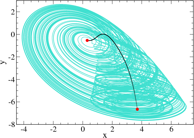
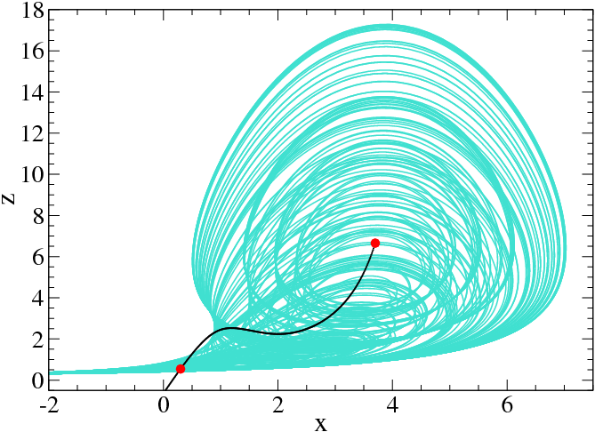
Figure 1: Connecting curve of the Rössler model. The curve intersects the attractor twice, as seen in the $x$-$z$ projection. Parameter values: $(a,b,c)=(0.556,2,4)$.

VII.2 Lorenz model

The purpose of the model established by Edward Lorenz Lore63 was initially to analyze the unpredictable behavior of weather. After having developed non-linear partial differential equations starting from the thermal equation and Navier-Stokes equations, Lorenz truncated them to retain only three modes. The most widespread form of the Lorenz model is as follows:

$$\overrightarrow{V}\left({{\begin{array}[]{*{20}c}{\dot{x}\hfill}\\ {\dot{y}\hfill}\\ {\dot{z}\hfill}\\ \end{array}}}\right)=\overrightarrow{\Im}\left({{\begin{array}[]{*{20}c}{f_{1}\left({x,y,z}\right)\hfill}\\ {f_{2}\left({x,y,z}\right)\hfill}\\ {f_{3}\left({x,y,z}\right)\hfill}\\ \end{array}}}\right)=\begin{pmatrix}{\sigma\left({y-x}\right)}\\ {Rx-y-xz}\\ {-bz+xy}\end{pmatrix}$$ (19)

where $\sigma$, $R$ and $b$ are real parameters. Once again, the connecting curves were computed using all three methods described in Sec. IV. The calculation using the third method was performed with Mathematica 7 (Files are available at: http://ginoux.univ-tln.fr). All methods gave the same curves.

Three connecting curves pass through the saddle at the origin: one corresponding to each of the three eigendirections with real eigenvalues. The simplest of these curves is the $z$-axis, which is simple to compute by hand. This particular curve is a trajectory of the Lorenz model. A second heads off to $z\rightarrow-\infty$ and has little effect on the attractor. The third connecting curve passes through all three fixed points. This curve is shown in Fig. 2 in both the $x$-$y$ and $y$-$z$ projections for $(R,\sigma,b)=(28,10,8/3)$. When $R$ is increased, the return flow from one side of the attractor to the other exhibits a fold and the connecting curve intersects the attractor at the fold. This reflects a similar property shown by the Rössler equations.

The connecting curves present additional constraints on the structure of the Lorenz attractor above and beyond those implied by the location and stability of the fixed points. Specifically, the flow spirals around and away from the connecting curve that passes through the two foci. In addition, the $z$ axis also provides some structure on this flow, as the flow also always passes in the same direction around this axis Byrn04 .

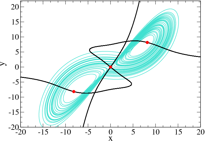
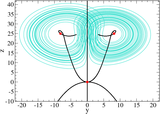
Figure 2: Connecting curve of the Lorenz model. One nontrivial connecting curve heads off to $z\rightarrow-\infty$ and has little effect on the structure of the attractor. The other nontrivial connecting curve connects all three fixed points, and is plotted extending through the foci. The third connecting curve is the $z$ axis. Parameter values: $(R,\sigma,b)=(28,10,8/3)$.

VII.3 Lorenz model of 1984

In 1984 Lorenz proposed a global atmospheric circulation model in truncated form Lore84 . The model consists of three ordinary differential equations:

$$\overrightarrow{V}\left({{\begin{array}[]{*{20}c}{\dot{x}\hfill}\\ {\dot{y}\hfill}\\ {\dot{z}\hfill}\\ \end{array}}}\right) = \overrightarrow{\Im}\left({{\begin{array}[]{*{20}c}{f_{1}\left({x,y,z}\right)\hfill}\\ {f_{2}\left({x,y,z}\right)\hfill}\\ {f_{3}\left({x,y,z}\right)\hfill}\\ \end{array}}}\right)$$ (26)

$$= \begin{pmatrix}{-y^{2}-z^{2}-a(x-F)}\\ {-y+xy-bxz+G}\\ {bxy+xz-z}\end{pmatrix}$$ (27)

In this model the variable $x$ represents the strength of the globally circling westerly wind current and also the temperature gradient towards the pole. Heat is transported poleward by a chain of large scale eddies. The strength of this heat transport is represented by the two variables $x$ and $y$, which are in quadrature. The control parameters $aF$ and $G$ represent thermal forcing. The parameter $b$ describes the strength of displacement of the eddies by the westerly current.

In Fig. 3 we show two projections of this attractor for control parameters $(a,b,F,G)=(1/4,4,8,1)$ as well as the connecting curve. For this set of parameter values there are three fixed points, only one of which is real at $(x,y,z)=(7.996,-0.00653,0.0298)$. It is clear that the connecting curve goes through the hole in the middle of the attractor, and that the attractor winds around part of the connecting curve where most of the bending and folding of the attractor occurs. The connecting curve in the $x$-$y$ projection passes through the fixed point off scale to the right.

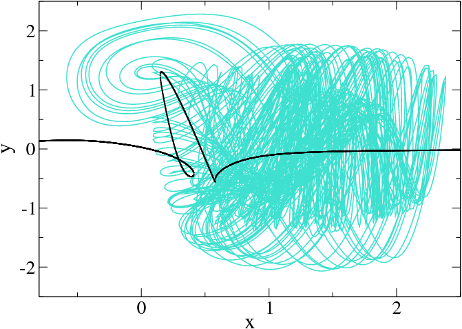
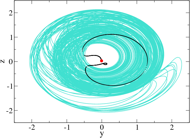
Figure 3: Strange attractor generated by the Lorenz global circulation model of 1984. The connecting curve threads through the inside of the attractor, and is caressed by the attractor where the stretching and folding is most pronounced. Parameter values: $(a,b,F,G)=(1/4,4,8,1)$.

VII.4 Rössler model of hyperchaos

Rössler proposed a simple four-dimensional model in 1979 to study hyperchaotic behavior Ross79 . This model is

$$\overrightarrow{V}\left({{\begin{array}[]{*{20}c}{\dot{x}\hfill}\\ {\dot{y}\hfill}\\ {\dot{z}\hfill}\\ {\dot{w}\hfill}\\ \end{array}}}\right) = \overrightarrow{\Im}\left({{\begin{array}[]{*{20}c}{f_{1}\left({x,y,z,w}\right)\hfill}\\ {f_{2}\left({x,y,z,w}\right)\hfill}\\ {f_{3}\left({x,y,z,w}\right)\hfill}\\ {f_{4}\left({x,y,z,w}\right)\hfill}\\ \end{array}}}\right)$$ (36)

$$= \begin{pmatrix}{-y-z}\\ {x+ay+w}\\ {b+xz}\\ {-cz+dw}\end{pmatrix}$$ (37)

Here the state variables are $(x,y,z,w)$ and the control parameters are $(a,b,c,d)$. The connecting curve was computed using methods 1 and 2 of Sec. IV. The first method gave very complicated results. Method 2 gave simpler results when the coordinate $z$ was used to express the behavior of the remaining four variables. The eigenvalue $\lambda$ was expressed as the root of a seventh degree polynomial equation whose coefficients were functions of the four control parameters $(a,b,c,d)$ and $z$. The remaining three coordinates were rational functions of small degree in the variables $z$ and $\lambda(z;a,b,c,d)$. Two projections of the hyperchaotic attractor and the connecting curve are shown in Fig. 4. The computation was carried out for $(a,b,c,d)=(1/4,3,1/2,1/20)$. The fixed points are shown as large dots along the connecting curve. It is clear from this figure that the connecting curve provides information about the structure of the attractor, as the flow in the attractor swirls around the connecting curve.

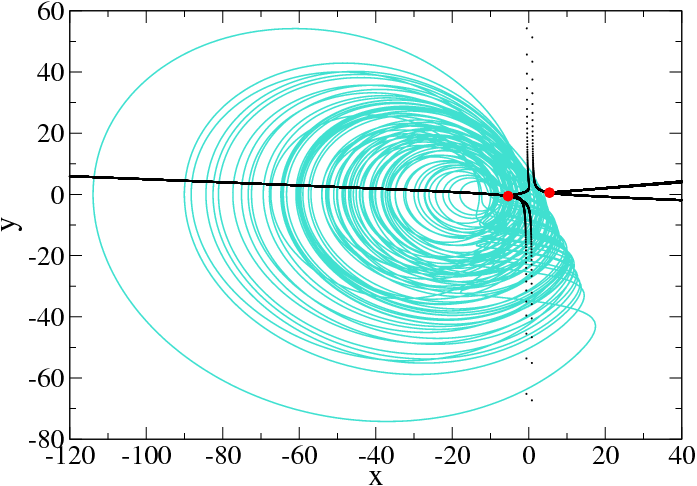
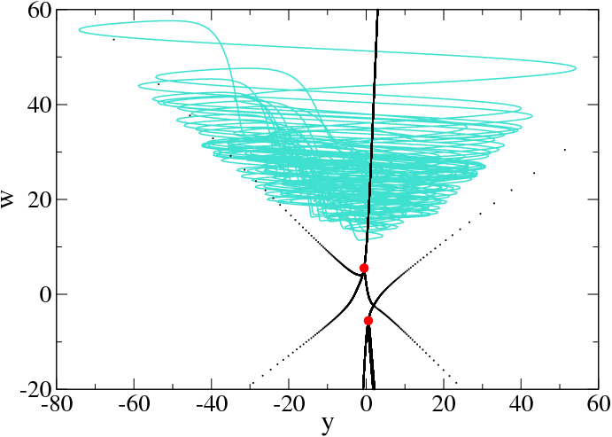
Figure 4: Hyperchaotic attractor generated by the 1979 Rössler model for hyperchaos. Parameter values: $(a,b,c,d)=(1/4,3,1/2,1/20)$.

VII.5 Thomas Model

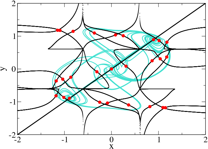
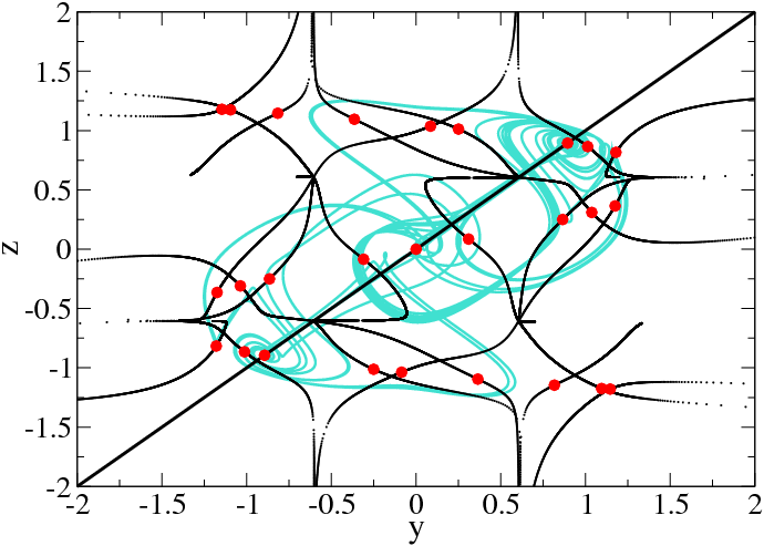
Figure 5: Connecting curves for the Thomas attractor. One connecting curve is the symmetry axis $x=y=z$. The remaining connecting curves exhibit the six-fold symmetry of the system and seek out the holes in the attractor. Parameter values: $(a,b)=(1.1,0.3)$.

Thomas proposed the following model of a feedback circuit with a high degree of symmetry Thom99 :

$$\overrightarrow{V}\left({{\begin{array}[]{*{20}c}{\dot{x}\hfill}\\ {\dot{y}\hfill}\\ {\dot{z}\hfill}\\ \end{array}}}\right) = \overrightarrow{\Im}\left({{\begin{array}[]{*{20}c}{f_{1}\left({x,y,z}\right)\hfill}\\ {f_{2}\left({x,y,z}\right)\hfill}\\ {f_{3}\left({x,y,z}\right)\hfill}\\ \end{array}}}\right)$$ (44)

$$= \begin{pmatrix}{-bx+ay-y^{3}}\\ {-by+az-z^{3}}\\ {-bz+ax-x^{3}}\end{pmatrix}$$ (45)

This set of equations exhibits the six-fold rotation-reflection symmetry $S_{6}$ about the $(1,1,1)$ axis. The symmetry generator is a rotation about this axis by $2\pi/6$ radians followed by a reflection in the plane perpendicular to the axis. The origin is always a fixed point and, for $a-b>0$, there are two on-axis fixed points at $x=y=z=\pm\sqrt{b-a}$. For $(a,b)=(1.1,0.3)$ there are 24 additional off-axis fixed points. These fall into four sets of symmetry-related fixed points (sextuplets). One point in each sextuplet is $(0.085,1.037,0.309),$ $(0.250,1.013,0.865),$ $(0.364,-1.095,1.175),$ $(1.146,-1.180,-0.816)$. The remaining points in a multiplet are obtained by cyclic permutation of these coordinates: $(u,v,w)\rightarrow(w,u,v)\rightarrow(v,w,u)$ and inversion in the origin $(u,v,w)\rightarrow(-u,-v,-w)$. The chaotic attractor for this dynamical system is shown in Fig. 5, along with the symmetry-related connecting curves and the 27 fixed points. One of the connecting curves is the rotation axis. This is an invariant set that connects the three on-axis fixed points. It therefore cannot intersect the attractor. In fact, this set has the same properties as the $z$-axis does for the Lorenz attractor of 1963 Byrn04 . The remaining connecting curves trace out the holes in the attractor. In this sense they provide additional constraints on the structure of the attractor over and above those provided by the spectrum of fixed points.

VIII Discussion

In this work we go beyond the zero-dimensional invariant sets (fixed points) that serve to a limited extent to define the structure of an attracting set of a dynamical system. We have introduced a curve that we call a connecting curve, since it passes through fixed points of an autonomous dynamical system. We have defined this curve in two different ways: dynamically and kinematically. It is defined a vortex core curve dynamically through an eigenvalue-like equation $J\vec{V}=\lambda\vec{V}$, where $\vec{V}(x)$ is the velocity vector field defining the dynamical system and $J_{ij}=\partial V_{i}/\partial x_{j}$ is its Jacobian. We have defined a connecting curve kinematically as the locus of points in the phase space where the principal curvature is zero. These two definitions are equivalent.

Three methods were introduced for constructing this curve for autonomous dynamical systems. They were applied to the standard Rössler and Lorenz attractors, where their behavior with respect to the attractors is shown in Figs. 1 and 2. In the figures shown for these attractors, it is clear that the flow rotates around the connecting curves, which therefore help to define the structure of the attractor. The connecting curves were also constructed for a later Lorenz model, the global atmospheric circulation model of 1984, and for a later model introduced by Rössler to study chaotic behavior in four dimensional phase spaces. Finally, a multiplicity of connecting curves was computed for an attractor with a high degree of symmetry, the Thomas attractor. This is shown in Fig. 5. The flows shown in Figs. 3, 4, and 5 are clearly organized by their connecting curves. In this sense the connecting curve provide additional important information about the structure of an attractor, over and above that provided by the number, nature, and distribution of the fixed points. A number of other connecting curves have been computed, and can be seen at http://www.physics.drexel.edu/~tim/programs/.

References

- (1) H. Poincaré, Sur les courbes définies par une équation differentielle, J. Math. Pures et Appl., Série III, 7, 375-422 (1881).
- (2) H. Poincaré, Sur les courbes définies par une équation différentielle, J. de Math Pures Appl., Série III, 8, 251-296 (1882).
- (3) H. Poincaré, Sur les courbes définies par une équation différentielle, J. Math. Pures et Appl., Série IV, 1, 167-244 (1885).
- (4) H. Poincaré, Sur les courbes définies par une équation differentielle, J. Math. Pures et Appl., Série IV, 2, 151-217 (1886).
- (5) M. Roth and R. Peikert, A higher-order method for finding vortex core lines, Proceedings IEEE of the conference on Visualization’98, 143-150 (1998).
- (6) E. A. Coddington and N. Levinson, Theory of Ordinary Differential Equations, NY: McGraw Hill, 1955.
- (7) M. Frechet, La notion de differentielle dans l’analyse generale. Annales scientifiques de l’Ecole Normale Superieure, Ser. 3, 42, 293-323 (1925).
- (8) J. M. Ginoux, Differential Geometry Applied to Dynamical Systems, World Scientific Series on Nonlinear Science, Series A, Vol. 66, Singapore: World Scientific, 2009.
- (9) J. M. Ginoux and R. Rossetto, Slow manifold of a neuronal bursting model, in: Understanding Complex Systems, Heidelberg: Springer-Verlag, 2006.
- (10) J. M. Ginoux, B. Rossetto and L. O. Chua. Slow Invariant Manifolds as Curvature of the flow of Dynamical Systems, Int. J. Bifurcation and Chaos, 11, 18, 3409-3430 (2008).
- (11) D. J. Struik, Lectures on Classical Differential Geometry, Dover: New York, 1961.
- (12) E. Kreyszig, Differential Geometry, New York: Dover, 1959.
- (13) A. Gray, S. Salamon, and E. Abbena, Modern Differential Geometry of Curves and Surfaces with Mathematica, London: Chapman & Hall/CRC, 2006.
- (14) S. Wilkinson, Intersection of surfaces, Mathematica in Education and Research, Volume 8, No. 2, Spring 1999.
- (15) O. E. Rössler, An equation for continuous chaos, Physics Letters A57(5), 397-398 (1976).
- (16) E. N. Lorenz, Deterministic nonperiodic flow, J. Atmos. Sci. 20, 130-141 (1963).
- (17) G. Byrne, R. Gilmore, and C. Letellier, Distinguishing between folding and tearing mechanisms in strange attractors, Phys. Rev. E70, 056214 (2004).
- (18) E. N. Lorenz, Irregularity: a fundamental property of the atmosphere, Tellus 36A, 98-110 (1984).
- (19) O. E. Rössler, An equation for hyperchaos, Physics Letters A31, 155-157 (1979).
- (20) R. Thomas, Deterministic chaos seen in terms of feedback circuits: Analysis, synthesis, “labyrinth chaos”, Int. J. Bif. Chaos 9(10), 1889-1905 (1999).