Nonlocal feedback in nonlinear systems

Abstract

A shifted or misaligned feedback loop gives rise to a two-point nonlocality that is the spatial analog of a temporal delay. Important consequences of this nonlocal coupling have been found both in diffusive and in diffractive systems, and include convective instabilities, independent tuning of phase and group velocities, as well as amplification, chirping and even splitting of localized perturbations. Analytical predictions about these nonlocal systems as well as their spatio-temporal dynamics are discussed in one and two transverse dimensions and in presence of noise.

1 Introduction

There is a considerable interest in dynamical regimes in which small fluctuations and ”noise” are amplified. In a large class of optical systems this behavior is caused by convective instabilities santagiustina97 ; taki00 . A convective instability happens in presence of some source of drift when a state of a nonlinear system becomes unstable and the group velocity of a localized perturbation is larger than the velocity of propagation of the instability front. As a result, in the laboratory frame the perturbation is amplified but moves away and eventually decays at any point in a finite spatial domain if it is not reflected at the boundary. The existence of these instabilities has been shown in systems in which the propagation of disturbances is characterized by drift or walk-off, modelled by a gradient term. For such systems small regions of convective instabilities have been predicted and observed in hydrodynamics ahlers83-gondret99 , plasma briggs physics, traffic flow  mitarai and optics santagiustina97 ; louvergneaux04a ; mussot08 .

It was recently shown that significantly larger windows of convective instabilities are induced by nonlocal terms in the governing equations papoff05a . In optics, these terms result from the presence of an off-axis or shifted feedback loop which is modeled by a two point nonlocality that is the spatial analogous of a temporally delayed feedback. This is a common experimental issue and has been subject of both theoretical and experimental study in liquid crystals light valves ramazza98a ; rankin03a ; pastur04a , Kerr-like media seipenbusch97a ; louvergneaux04a ; agez06a and generic nonlinear systems with diffusive papoff05a and diffractive zambrini07a coupling. We note that the importance of feedback loops goes well beyond the realm of optics arecchi99a and has been long recognized in other fields of physics and also in biology and engineering kitano01a ; franklin02a . Usually feedback loops are introduced to better control the system and to limit the growth of noise, while in the papers quoted a nonlocal feedback has been used mainly to study fundamental properties of fluctuations in non linear systems when convective instabilities are induced. In a recent experiment, however, an off-axis feedback loop has been used very effectively to suppress noise-sustained structures caused by an intrinsic drift term in a free electron laser evain09a , showing that two-point nonlocality are not only fundamentally interesting, but also extremely useful.

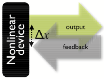
Figure 1: Schematic representation of a nonlinear device with shifted feedback. The output beam is re-injected into the device after a shift $\Delta x$.

In this paper we review the effect of off-axis feedback in a broad class of optical devices and explore the effect of the two-point nonlocality in the case of two transverse dimensions. We consider passive as well as active nonlinear media with fast decay of the polarization coullet89a , including media with negative refraction index kockaert06a ; hoyuelos and devices with soft apertures dunlop97b . Within the media we consider both diffusion and diffraction and show how an off-axis feedback changes the nature of the first instability threshold. As a consequence, there are large windows of control parameters where small localized signals can be strongly amplified while the background radiation in other region of the system remains very low zambrini07a . The amplification does not need a continuous signal injection and takes place even when the initial perturbation is switched off. Furthermore, in systems with diffraction and active media, the signal moves across the cavity with transverse phase and group velocities that are easily managed to have the same or opposite signs zambrini07a . In spite of the broken transverse reflection symmetry, localized perturbations can move both towards or against the off-set direction and can even split into two counter-propagating components, with the laser operating as a signal splitter. Both noise sustained structures and signals control are shown by numerical simulations of the full nonlinear model confirming our theoretical analysis and a rich spatio-temporal dynamics. Previous analysis of Refs. zambrini07a ; papoff09b are extended considering two transverse spatial dimensions.

2 Equations

Off-axis feedback loops, in which the propagation of light is guided, are used with nonlinear phase/amplitude modulators in which material evolves much more slowly than the electric field and its polarization. First examples were liquid crystal light valves with feedback signal propagating through fibers whose position was easily controlled ramazza98a ; rankin03a ; pastur04a . These devices -in presence of a shifted feedback- are modelled by equations of the type papoff05a ; zambrini06a

$$\partial_{t}\varphi=\nabla^{2}_{\perp}\varphi+f_{1}(\varphi;\mu)+f_{2}(\varphi_{\Delta x};\mu).$$ (1)

$\varphi(x,y,t)$ is a real field that represents the state of the material - for liquid crystal based devices it is related to the alignment of the molecules - at a point $(x,y)$ and time $t$, while $\varphi_{\Delta x}$ is evaluated at point $x+\Delta x$ and time $t$, respectively scaled with diffusion length and diffusion time. The control parameter $\mu$ is independent on $x$ for the sake of simplicity. $f_{1}$, $f_{2}$ are real functions that can be derived with respect to $\varphi$. In the limit of infinitely extended systems, the homogeneous states are solutions of $f_{1}+f_{2}=0$ and their domains of existence depend upon $\mu$ but not upon $\Delta x$.

A similar feedback is used also with active materials inside optical cavities. When the dynamics of the difference of the populations of the energy levels coupled to the light and of the polarization of the materials is much faster than the dynamics of the electric field, these systems are described by a single equation of the type zambrini07a ; papoff09b

$$\partial_{t}E=f(|E|^{2};\mu)E+de^{i\delta}\nabla^{2}_{\perp}E+re^{i\phi}E_{\Delta x}.$$ (2)

Here $E$ is the slowly-varying amplitude of the electric field within a scalar description, $d\cos{\delta},d\sin{\delta}$ are the diffusion and diffraction coefficients ($d>0$)and $\mu$ is a control parameter. Devices where only the polarization evolves much faster than the electric field are instead modelled by

$$\partial_{t}E = g_{1}(|E|^{2},N;\mu)E+de^{i\delta}\nabla^{2}_{\perp}E+re^{i\phi}E_{\Delta x},$$ (3)

$$\partial_{t}N = g_{2}(|E|^{2},N,\nabla^{2}_{\perp}N;\mu),$$

where $N$ represent the internal dynamics of the material coupled with light. We consider feedback loops in which the time delay $\Delta t$ is very small compared to the time scale of the slowly varying envelope of the field. The feedback can then be characterized by an amplitude $0<r<1$ and a phase shift $\phi=\omega_{L}\Delta t$, where $\omega_{L}$ is the carrier frequency and couples the field $E$ in $(x,y)$ with the field $E_{\Delta x}$ in a shifted point. $f$, $g_{1}$ and $g_{2}$ are nonlinear complex functions that can be derived with respect to $E$ and $N$. The trivial solutions of Eq. (2) and Eqs.(3) are $E=0$, and $E=0$, $N=N_{0}$, respectively. Interestingly, our analysis applies also to equations with the more general feedback term $[f_{1}(|E|^{2})E]_{\Delta x}$, with $re^{i\phi}=f_{1}(0)$.

We are interested in the dynamics of perturbations $\delta E\sim\exp{(\omega t+i{\bf k}\cdot{\bf x})}$ around the uniform states in the linear regime. The dynamics of perturbations for Eq.(2) and Eqs.(3) is contained in the dispersion relation

$$\omega=\beta-e^{i\delta}(k_{x}^{2}+k_{y}^{2})+re^{i(\phi+k_{x}\Delta x)},$$ (4)

where space is rescaled in units of $\sqrt{d}$. Here $\beta=f(0)$ for Eq.(2) and $\beta=g_{1}(0,N_{0})$ for Eqs.(3). For class B models, perturbations $\delta N$ are always damped and decoupled from $\delta E$ and can be ignored.

We note that Eq.(4) with $\delta=0$, $\beta=\partial_{\varphi}f_{1}$, $r=|\partial_{\varphi}f_{2}|$ and $\phi=0$ or $\pi$ depending on the sign of $|\partial_{\varphi}f_{2}|$, is the dispersion relation for the perturbations of the uniform states of Eq.(1). This shows that despite the different physical meaning of the variables $\varphi$ and $E$, as well as the significant differences in the characteristic time scales and in the light-matter coupling behind Eq.(1) and Eq.(2) or Eqs.(3), the dynamics of the perturbations of Eq.(1) is a special case of the dynamics of the perturbations of the other two cases.

From Eq.(4) we find that there are unstable band of ${\bf k}=(k_{x},k_{y})$ with the most unstable ones given by

$$\nabla_{k}\omega_{R} = -(2k_{x}\cos{\delta}+r\Delta x\sin{(k_{x}\Delta x+\phi)},2k_{y}\cos{\delta})$$ (5)

$$= (0,0)$$

$$\partial^{2}_{k_{x}^{2}}\omega_{R} = -(2\cos{\delta}+r\Delta x^{2}\cos{(k_{x}\Delta x+\phi)})<0,$$ (6)

$$\partial^{2}_{k_{y}^{2}}\omega_{R} = -2\cos{\delta}<0.$$ (7)

The subscripts $R$ and $I$ refer to real and imaginary part, respectively. The conditions (6-7) ensure that the solution of Eq.(5) corresponds to the perturbation with the largest amplification; note that Eq.(7) is the standard stability condition for diffusive equations.

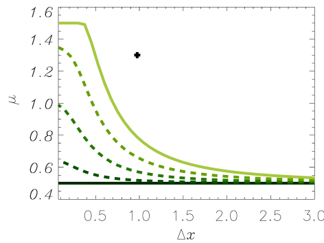
Figure 2: Instability threshold as a function of the shift. The control parameter $\mu=\beta_{R}+1$ is represented for easy comparison with results in the following section. The effect of the feedback phase on the instability is shown: thresholds for $\phi=0$ (horizontal dark line) and increasing values $\phi=\pi/4,\pi/2,3\pi/4,\pi$ (lighter colors), $\delta=0.49\pi$, $r=0.5$. The dot corresponds to the parameter choice in Fig. 5.

An important feature of the instability threshold is that it is a function of four relevant parameters, namely $\phi,\delta,r\Delta x^{2}$, and $\beta_{R}\Delta x^{2}$, and is independent on $\beta_{I}$; therefore increasing the shift size $\Delta x$ produces on the device the same effect of larger gain $\beta_{R}$ and feedback $r$. A specific effect of the nonlocality is that the relative strength of diffusion and diffraction, $\delta$, also becomes an effective parameter to control the threshold position. For active materials, the lowest gain and feedback thresholds are generally found in the purely diffractive limit ($\delta\sim\pi/2$). The threshold value for the scaled feedback strength $r\Delta x^{2}$ is independent on the sign of the refractive index (sign of $\delta$) and increases with diffusion. Both $\beta_{R}$ and $r$ can be increased to cross the laser threshold and –similarly to the case of perfect alignment– if the feedback is out of phase then stronger gain is required, as shown in Fig. 2. For vanishing shift ($\Delta x=0$) this phase acts as a detuning and increases the threshold while for larger shift values the threshold tends asymptotically to the value for in-phase feedback ($\phi=0$). Quite surprisingly, a misalignment lowers the threshold because the most unstable mode has $k_{x,I}\neq 0$ and, in this case, the nonlocal coupling can reduce the feedback dephasing. Consistently with this interpretation, when the feedback perfectly in phase with the intracavity field ($\phi=0$) the most unstable mode is homogeneous with $k_{x,I}=0$ and the threshold is independent on the lateral shift $\Delta x$.

The dispersion Eq. (4) has in general a not vanishing imaginary part corresponding to a non null phase velocity

$${\bf v}_{p} = -\omega_{I}({\bf k})\frac{{\bf k}}{|{\bf k}|^{2}}=$$

$$- [\beta_{I}-(k_{x}^{2}+k_{y}^{2})\sin{\delta}+r\sin{(k_{x}\Delta x+\phi)}]\frac{{\bf k}}{|{\bf k}|^{2}},$$

For the most unstable ${\bf k}$, ${\bf k}_{c}$, the phase velocity is

$${\bf v}_{p}({\bf k}_{c})=({k_{x}}_{c}\sin{\delta}-\frac{\beta_{I}}{{k_{x}}_{c}}+\frac{2\cos{\delta}}{\Delta x},0),$$ (9)

and group velocity is

$${\bf v}_{g}({\bf k}_{c}) = \nabla_{k}\omega_{I}({\bf k}_{c})=$$ (10)

$$(2{k_{x}}_{c}\sin{\delta}-r\Delta x\cos{({k_{x}}_{c}\Delta x+\phi)},0)=$$

$$(2{k_{x}}_{c}\sin{\delta}\mp\sqrt{1-\frac{4{k_{x}}_{c}^{2}\cos{\delta}^{2}}{r^{2}\Delta x^{2}}},0).$$

Note that both ${\bf v}_{p}({\bf k}_{c})$ and ${\bf v}_{g}({\bf k}_{c})$ are null in the direction orthogonal of the shift and coincide with the one dimensional values. In Eq. (10) the $-$ sign solution always satisfies Eq.(6) and therefore corresponds to a wave-packet with frequency spectrum centered on a local maximum of the amplification. On the contrary, the $+$ sign may not satisfy Eq.(6). We remind that Eqs.(9-10) with $\delta=0$, $\phi=0$ or $\phi=\pi$ give the velocities for the diffusive systems of Eq.(1). An example of the large variability of phase and group velocities at the critical wave-number are shown in Fig. 3.

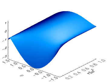
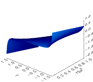
Figure 3: Variation of phase (upper plot) and group (lower plot) velocies, $v_{p,x}(k_{c})$ and $v_{g,x}(k_{c})$ respectively, depending on $\delta$ and $r\Delta x^{2}$. Other parameters: $\beta=0.2-i0.02$ and $\phi=\pi/4$.

The analysis above shows that the phase velocity at ${\bf k}_{c}$ and the group velocity are always parallel to the shift, while their sign varies. There are manifolds in the control parameter space that separate regions in which the group and the phase velocity of the most unstable perturbation have the same sign from region in which these velocities have opposite sign. Moreover, the real part of the dispersion relation may have more than one maximum, so that a single perturbation may split into two wave-packets. The independent tunability of phase and group velocity is a specific feature of optical systems with two-point nonlocality: as a matter of fact, gradient terms fix both velocities in the same direction of the drift, while two-point nonlocality in diffusive systems gives always opposite velocities at the critical wavenumber ($v_{p}({\bf k_{c}})=-v_{g}({\bf k_{c}})$).

In the purely diffractive limit $\delta\rightarrow\pi/2$, both velocities are actually odd functions of $k_{c}$; this symmetry is reduced by the effect of diffusion ($|\delta|<\pi/2$). Therefore, even if for $\phi=\pi$ both $+k_{c}$ and $-k_{c}$ are unstable, from the linear analysis we do not expect intensity stripes above threshold in such optical systems. As a matter of fact, the instability of these two states (different traveling waves) is rather peculiar and opens the possibility of bistability instead of stripe pattern formation.

Note that the tunability of transverse phase and group velocities is a general property that is valid also in the case in which $\Delta t$ is of the order of the time scale of the slowly varying amplitude papoff09b . This tunability is therefore a rather robust and distinctive feature of two-point nonlocality with respect to models where velocities are induced by drift terms zambrini06a . We remark that the parameters $\phi$ and $\delta$ are essential for this tunability: for this reason in the diffusive systems of Eq.(1) the tunability is absent and the phase and group velocities have always opposite sign.

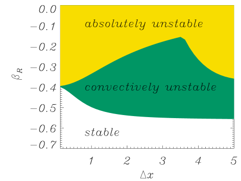
Figure 4: Regimes in which the homogeneous solution is stable, convectively unstable and absolutely unstable as a function of the shift and for $\delta=0.45\pi$, $r=0.56$, $\phi=0.25\pi$.

We now consider whether the perturbations with non null group velocities grow fast enough to occupy the entire system (absolute instability) or if their group velocity is such that the perturbations, although growing, move away (convective instability).

The analysis is performed in an infinite system evaluating the asymptotic behavior of perturbations both in a traveling and in a fixed reference frame. Note that the distinction between absolutely and convectively unstable regimes is generally given in infinite system while the inclusion of boundary effect in finite systems can change, in some case even drastically, the instability scenario. The simpler example is the case of periodic boundary conditions: in this case no convective instability does exist at all. Another interesting related question for finite systems is the phenomenon of transient growth of perturbations observed in cases where the linear stability operator is non normal, i.e. does not commute with its adjoint papoff08a . The connection between convective instability and transient growth of perturbations is still an open question chomaz . What has been characterized is the macroscopic amplification of quantum noise in optical systems in this regime zambrini02 .

We determine absolute thresholds by evaluating asymptotically the Green function: we extend analytically the dispersion relation to complex wavevectors $k$ (for one transverse dimension) and find the appropriate integration paths in the plane $k$. A detailed analysis is given in papoff09b , here we remark only that the for the purely diffusive systems of Eq.(1) the asymptotic evaluation of the Green function is done by closing the integration contour using only equiphase lines from saddle points. Furthermore, it turns out that the absolute threshold is determined only by the saddle closest to the imaginary axis. For Eq.(2) and Eqs.(3) instead, we close with steepest descent paths a finite segment $[{k_{I}}_{m},{k_{I}}_{M}]$ of the imaginary axis containing all the $k_{I}$ with $w_{R}(0,k_{I})>0$ and with ${k_{I}}_{m}$, ${k_{I}}_{M}$, such that $w_{R}(0,k_{I})<0$ for $k_{I}\leq{k_{I}}_{m}$ and $k_{I}\geq{k_{I}}_{M}$. For these two cases, the correct determination of the absolute thresholds requires to identify the integration paths and to evaluate the contribution to the Green functions of the saddle points that are part of it, excluding all the others.

Summarizing, our analysis allows to distinguish three regimes both in diffusive papoff05a and laser zambrini07a systems with a two-point nonlocality, as shown in Fig. 4 for a particular parameters choice. The homogeneous (vanishing or non-lasing) state becomes unstable above a first threshold (convectively unstable regime) corresponding to positive dispersion Eq.(4). The absolutely unstable regime is found only after evaluation of the asymptotical growth of perturbations, involving an integral whose approximate value is found with a non-trivial application of the saddle-point technique. This calculation is fully described in zambrini07a and papoff09b and here we only stress that not monotonic threshold dependence on the shift can be found (Fig. 4) and have been also checked by numerical simulations of dynamical equations.

3 Nonlinear and stochastic spatio-temporal dynamics

The general analysis of the previous section encompasses a broad class of non-diffractive as well as laser models. Main features of the spatio-temporal dynamics of specific systems can be anticipated from the linear stability analysis and we will see some examples in the case of a class A jakobsen94a laser:

$$\frac{\partial}{\partial t}E = -E(1+i\theta-N)+e^{i\delta}\nabla_{\perp}^{2}E+re^{i\phi}E(x+\Delta x,y)+$$

$$\epsilon\xi(x,y,t)$$

$$N = \frac{\mu}{1+|E|^{2}}$$ (11)

with $\xi(x,y,t)$ complex Gaussian white noise. Numerical simulations of this nonlinear model are performed with a second-order in time Runge-Kutta method and using the random number generator of Ref. Toral93 . The connection with the analysis of the previous section is given by $\beta=\mu-1-i\theta$. Numerical simulations confirm the predicted instability diagram; the wavenumbers dynamically selected and the velocities are well approximated by those obtained from the analytical analysis of the linear dispersion.

3.1 Signal splitting and interactions

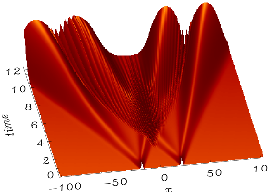
Figure 5: Spatio-temporal $intensity$ dynamics showing the interaction of signals in a 1D class A laser with parameters $\Delta x=1$, $\mu=1.3$, $\theta=-1$, $\delta=0.49\pi$, $r=0.5$ , $\phi=\pi$, $\epsilon=0$ (see Fig. 2). Evolution starting from two small Gaussian perturbations as can be recognized in the picture at time $t=0$.

The regime of convective instability allows the amplification of localized light signals below the lasing threshold. The direction of propagation of these signals depends on the group velocity Eq. (10) and steering can be obtained also non-mechanically by varying the feedback loop phase, as shown in Figs. 3 and 4 of Ref. zambrini07a . Particularly interesting is the case in which the feedback is negative, $\phi=\pi$, first discussed in Ref. zambrini07a . The recovered symmetry in the dispersion relations gives rise to instability of both positive and negative wave-vectors and, as a peculiar consequence of the two-point nonlocality, these waves propagate in opposite directions. This allows the system to operate as a signal splitter in which an initial perturbation, such as a localized spot of light, is divided into two counter-propagating copies. This phenomenon is robust also in presence of noise papoff09b and deviations from the symmetry, i.e. differences between the left and the right propagating signals, are due to nonlinear effects zambrini02 ; zambrini05 .

Once excited, these localized signals are amplified and propagate in the system (even in opposite directions) without giving rise to any intensity modulation, even if the field is actually spatially oscillating. We will now focus on a different aspect of signal control, namely signal interaction when they cross each-other. As localized perturbations are split into counter-propagating ones it is actually possible to have signals crossing during temporal evolution. This case is represented in Fig. 5. In this example the system is excited in two separated points at an initial time and the dynamics is considered in the case of only one transverse dimension. We see that two of the four generated signals cross and locally interfere generating a transient intensity stripe in the center of Fig. 5. Moreover, looking on the left (right) side, we see that due to the different velocities of perturbations fronts, the trailing edge of the left signal is reached by the leading edge of the following signal and this also generates intensity modulation by interference. Finally, after a transient time (not shown in Fig. 5) and as expected, due to the convective character of the instability, the system evolves locally back to the homogeneous vanishing state.

3.2 Patterns in one and two dimensions

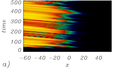
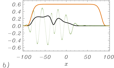
Figure 6: (a) Spatio-temporal evolution of the intensity field for one transverse dimension and starting from a noisy initial condition. (b) Intensity $|E(x,t=100)|^{2}$ (black line), real part (green dotted line) of the field, and pump profile $\mu$ (orange line). Parameters: $\Delta x=2$, $\theta=0$, $\delta=0.45\pi$, $r=0.56$ , $\phi=\pi/4$, $\epsilon=10^{-3}$. Super-Gaussian profile of $\mu$ with maximum value $0.6$.

In previous works we described the spatio-temporal dynamics of class A lasers assuming a one dimensional transverse geometry zambrini07a ; papoff09b . Good agreement with the theoretical predictions (threshold position, pattern wave-length, phase and group velocity) was found when considering rather $large$ systems where boundary conditions effects are negligible. The importance of the boundaries is particularly evident in the convectively unstable regime. In Fig. 6 we show the evolution of a noise sustained structure for $\delta=0.45\pi$, $r=0.56$, $\phi=0.25\pi$ and super-Gaussian pump with maximum value $\mu=0.6$ in the central region (see Fig. 6b). From Fig. 4 and remembering that $\beta_{R}=\mu-1$, we see that for these parameters the nonlasing state is convectively unstable and the field in Fig. 6a) has the typical incoherent profile discussed in papoff09b . Here we show that a large system is needed in order to observe noise sustained structures intensities in the system: the intensity represented in Fig. 6b is significantly high only in half of the system, far from the right edge of the pump profile $\mu$. In other words, the intensity growth –in this case against the shift direction– is rather slow and large systems are needed to observe an intense noise sustained pattern. Oscillations appear in the field profile (phase pattern given by the green line in Fig. 6b).

In order to give a representation of the aspect of spatial structures as they would appear in experiments with broad area lasers, it is interesting to consider the evolution of two-dimensional field $E(x,y,t)$. In Fig 7 we represent both fields profiles and intensities for the same parameters as in Fig. 6, showing the aspect of a noise sustained structure in the convective regime.

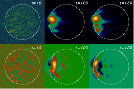
Figure 7: Temporal evolution of the intensity (upper line) and of the real part (lower line) of the field starting from a noisy initial condition. Parameters: $\Delta x=2$, $\theta=0$, $\delta=0.45\pi$, $r=0.56$ , $\phi=\pi/4$, $\epsilon=10^{-3}$. Super-Gaussian profile of $\mu$ with maximum value $0.6$ inside the circular area. For this value of $\mu$ the vanishing state is convectively unstable.

Three snapshots give an example of the dynamic character of this structure: numerical simulations in presence of noise show an incoherent traveling structure whose aspect is continuously changing.

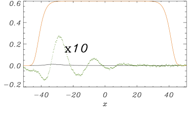
Figure 8: Section plot of the 2D intensity (black line) and real part (green dotted line) of the field for $t=100$. The corresponding values are multiplied by a factor 10 to be compared with the pump profile $\mu$ (orange line). Same parameters of Fig. 7.

The importance of the boundary and system size in this case is evident as it leads to a very low intensity noise sustained structure. Due to the reduced size of the pumped area with respect to previous 1D numerical simulations (compare $\mu$ super-Gaussians in Figs. 6 and 8) the intensity profile is dominated by a smooth front emerging on the right side and remains very small.

When the pump is increased this front becomes steeper and and a uniform intensity state occupies a broad part of the system. Above the absolutely unstable threshold a coherent phase pattern arises as shown in Fig. 9 and the system is in the lasing state.

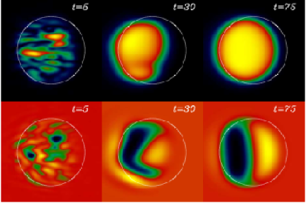
Figure 9: Temporal evolution of the intensity (upper line) and of the real part (lower line) of the field for vanishing state absolutely unstable. Parameters: $\Delta x=2$, $\theta=0$, $\delta=0.45\pi$, $r=0.56$ , $\phi=\pi/4$, $\epsilon=10^{-5}$. Super-Gaussian profile of $\mu$ with maximum value $1$.

Starting from a noisy initial condition, perturbations are washed away from the system and the intensity profile becomes intense and uniform. Also the coherence of the underlying phase pattern increases (in this case the pattern aspect ratio is very small and only one oscillation is actually seen in Fig. 9). Note also that the intensity profile is deformed and displaced against the direction of the shift, i.e. it is not exactly centered in the pumped region (white circle in Fig. 9, panels at $t=75$).

The most peculiar patterns in lasers with nonlocal feedback occur for $\phi=\pi$, when the system operates as a signal splitter. The change in the pattern aspect when increasing the pump is shown in Fig. 10. In the convectively unstable regime (two panels with $\mu=1.4$) there are now two regions of larger intensity, as perturbations with opposite wave-numbers travel apart, as expected. Intense light spots correspond to a certain coherence in the underlying phase pattern, while the intensity drops down where there are defects in the phase stripes. Intensity reaches larger values on one side (here the left one, against the positive shift direction, $\Delta x=2$) zambrini07a ; papoff09b ; zambrini05 .

Noise sustained patterns for negative feedback are then characterized by off-axis spots and have a vanishing intensity in the central area, while crossing the absolute instability threshold an intense and uniform profile is reached -after a transient- in the whole pumped region. Note that the phase pattern has larger wave-numbers in the noise sustained structure. After a longer transient (not shown in the picture) the stripe in the absolutely unstable regime (Fig. 10 for $\mu=2.1$) becomes orthogonal to the shift direction, as theoretically predicted.

Figure 10: Spatial distributions of the intensity (left panels) and field real part (right panels) for numerical simulations with super-Gaussian pump profiles with maximum intensity $\mu=0.7,1.4$, and $2.1$ inside the circular panels. In the external region the gain vanishes. Other parameters are $\Delta x=1$, $\theta=0.2$, $\delta=0.49\pi$, $r=0.5$ , $\phi=\pi$, $\epsilon=10^{-5}$. Simulations are started from noise initial condition.

3.3 Conclusions

Two-point nonlocality can be easily induced in optical devices through a displaced feedback loop and leads to distinctive effects opening interesting possibilities in experiments in extended devices. We have presented its analytical characterization through linear approximations, allowing to predict instability convective and absolute thresholds, unstable wave-numbers and velocity of drifting packets, in a broad class of two-dimensional nonlinear systems. Many differences with respect to the most studied drift, modelled by a gradient term, make this two-point nonlocality an interesting and versatile tool in view of experiments. In particular, such nonlocality opens significantly larger windows of control parameters where the system output state is sustained by the presence of noise instead of the dynamics (convective regime). In such regime the system can be locally excited generating a signal that is amplified during propagation. Note that the amplification here considered occurs once the (initial) local perturbation is removed, at difference of laser amplification above transparency, generally considered in presence of a continuous signal injection.

Another distinctive feature of displaced feedback and two-point nonlocality is the possibility to independently tune phase and group velocity, while gradient terms fix both velocities in the same direction of the drift. In optical systems such velocities have been shown to be either parallel or opposite and can be tuned even non-mechanically through the feedback phase $\phi$ (without touching the experiment alignment). Such large tunability is a characteristic of optical systems, while two-point nonlocality in diffusive systems gives always opposite velocities at the critical wavenumber ($v_{p}({\bf k_{c}})=-v_{g}({\bf k_{c}})$). Another distinctive feature of two-point nonlocality in optical systems is the possibility to control the feedback phase to operate the laser as a signal splitter (for $\phi=\pi$). Then an initial perturbation is split in two copies amplifying (even when the injection is removed) during their propagation in opposite directions through the broad area device.

In general, no oscillations are observed in the intensity profile and only phase patterns are present in lasers here considered. The interaction of traveling signals, however, displays also intensity modulation in the interaction region, as discussed in Sect. 3.1. Similarly, if instead of initial localized perturbations the system is considered in presence of noise, a central area of intensity stripes can be observed in a laser as shown in Fig. 10 of Ref. papoff09b . Numerical simulations considering only one transverse dimension allow to easily visualize the spatio-temporal dynamics, as in the case of the signals interactions in Fig. 5, or to see the spatio-temporal coherence of noise sustained structures, as in Fig. 6. On the other hand, simulations in two transverse dimensions here presented are important in view of experimental realizations, showing pattern features in the shift direction and in the orthogonal one. Examples are the orientation of phase oscillations, the elongated aspect of transients domains, as well as the displacement of lasing state with respect to the pumped region, as shown in Sect. 3.2. A last important aspect to be considered in view of experiments is the system size: analytical predictions for infinite systems are in quantitative agreement with simulations for relatively large systems, while a finite system effects gives important deviations in small systems not only when few oscillations of the phase patterns are present but also in the cases in which smooth fronts modulate the light intensity profile.

Funding from FISICOS (FIS2007-60327) and CoQuSys (200450E566) is acknowledged.

References

- (1) M. Santagiustina, P. Colet, M. San Miguel, D. Walgraef, Phys. Rev. Lett. 79 3633 (1997); Phys. Rev. E 58, 3843 (1998); Opt. Lett. 23, 1167 (1998).
- (2) M. Taki, N. Ouarzazi, H. Ward, P. Glorieux, JOSA B 17, 997 (2000).
- (3) J M. Chomaz, Phys. Rev. Lett. 69 (1992) 1931; K. L. Babcock, G. Ahlers, and D. S. Cannell, Phys. Rev. Lett. 67 (1991) 3388; Instability P. Gondret, P. Ern, L. Meignin, M. Rabaud, Phys. Rev. Lett. 82 (1999) 1442.
- (4) R. J. Briggs, Electron-Stream Interaction with Plasmas (MIT, Cambridge, MA, 1964)
- (5) N. Mitarai and H. Nakanishi, Phys. Rev. Lett. 85, 1766 (2000).
- (6) E. Louvergneaux, C. Szwaj, G. Agez, P. Glorieux, and M. Taki, Phys. Rev. Lett. 93 (2004) 101801.
- (7) A. Mussot, E. Louvergneaux, N. Akhmediev, F. IT, Boston, Reynaud, L. Delage, and M. Taki, Phys. Rev. Lett. 101 (2008) 113904.
- (8) F. Papoff and R. Zambrini, Phys. Rev. Lett. 94 (2005) 243903.
- (9) P. Ramazza, S. Ducci, and F. Arecchi, Phys. Rev. Lett. 81 (1998) 4128 .
- (10) S. Rankin, E. Yao, and F. Papoff, Phys. Rev. A 68 (2003) 013821.
- (11) L. Pastur, U. Bortolozzo, and P. Ramazza, Phys. Rev. E 69 (2004) 016210.
- (12) J. P. Seipenbusch, T. Ackemann, B. B. B. Schäpers, and W. Lange, Phys Rev. A 56 (1997) R4401.
- (13) G. Agez, P. Glorieux, M. Taki, and E. Louvergneaux, Phys. Rev. A 74 (2006) 043814.
- (14) R. Zambrini and F. Papoff, Phys. Rev. Lett. 99 (2007) 063907.
- (15) F. Arecchi, S. Boccaletti, and P. Ramazza, Physics Reports 318 (1999) 1.
- (16) Foundations of Systems Biology, edited by H. Kitano, MIT, Boston, 2001.
- (17) G. F. Franklin et al., Feedback Control of Dynamic Systems, Prentice Hall, 2002.
- (18) C. Evain, C. Szwaj, S. Bielawski, M. Hosaka, A. Mochihashi, M. Katoh, and M.-E. Couprie, Phys. Rev. Lett. 102, (2009) 134501
- (19) P. Coullet, L. Gill, and F. Rocca, Opt. Comm. 73 (1989) 403.
- (20) P. Kockaert, P. Tassin, G. V. der Sande, I. Veretennicoff, and M. Tlidi, Phys. Rev. A 74 (2006) 033822.
- (21) D. A. Martin, M. Hoyuelos, Phys. Rev. E 80 (2009), 056601.
- (22) A. Dunlop, W. Firth, and E. Wright, Opt. Commun. 138 (1997) 211.
- (23) F. Papoff and R. Zambrini, Phys. Rev. A 79 (2009) 033811
- (24) R. Zambrini and F. Papoff, Phys. Rev. E. 73 (2006) 016611.
- (25) F. Papoff, G. D’Alessandro, and G.-L. Oppo, Phys. Rev. Lett. 100 (2008) 123905; G. D’Alessandro, C.B. Laforet, Opt. Lett. 34 (2009) 614; G. D’Alessandro,F. Papoff, Phys. Rev. A 80 (2009) 023804.
- (26) C. Cossu and J. M. Chomaz, Phys. Rev. Lett. 78 (2007) 4387.
- (27) R. Zambrini and M. S. Miguel, Phys. Rev. A 66 (2002) 023807, R. Zambrini, S. Barnett, P. Colet, and M. S. Miguel, Phys. Rev. A 65 (2002) 023813.
- (28) R. Zambrini, M. S. Miguel, C. Durniak, and M. Taki, Phys. Rev. E 72 (2005) 025603(R).
- (29) P. K. Jakobsen, J. Lega, Q. Feng, M. Staley, J. V. Moloney, and A. C. Newell, Phys. Rev. A 49 (1994) 4189.
- (30) R. Toral and A. Chakrabarti, Comput. Phys. Commun. 74 (1993) 327.