Capillary instability in concentric-cylindrical shell: numerical simulation and applications in composite microstructured fibers

Abstract

Recent experimental observations have demonstrated interesting instability phenomenon during thermal drawing of microstructured glass/polymer fibers, and these observations motivate us to examine surface-tension-driven instabilities in concentric cylindrical shells of viscous fluids. In this paper, we focus on a single instability mechanism: classical capillary instabilities in the form of radial fluctuations, solving the full Navier–Stokes equations numerically. In equal-viscosity cases where an analytical linear theory is available, we compare to the full numerical solution and delineate the regime in which the linear theory is valid. We also consider unequal-viscosity situations (similar to experiments) in which there is no published linear theory, and explain the numerical results with a simple asymptotic analysis. These results are then applied to experimental thermal drawing systems. We show that the observed instabilities are consistent with radial-fluctuation analysis, but cannot be predicted by radial fluctuations alone—an additional mechanism is required. We show how radial fluctuations alone, however, can be used to analyze various candidate material systems for thermal drawing, clearly ruling out some possibilities while suggesting others that have not yet been considered in experiments.

I Introduction

The classical capillary instability, the breakup of a cylindrical liquid thread into a series of droplets, is perhaps one of the most ubiquitous fluid instabilities and appears in a host of daily phenomena Eggers1997 ; deGennes2002 from glass-wine tearing Cabazat92 , and faucet dripping to ink-jet printing. The study of capillary instability has a long history. In 1849, Plateau attributed the mechanism to surface tension: the breakup process reduces the surface energy Plateau1849 . Lord Rayleigh pioneered the application of linear stability analysis to quantitatively characterize the growth rate at the onset of instability, and found that a small disturbance is magnified exponentially with time Rayleigh1878 . Subsequently, Tomotika investigated the effect of viscosity of the surrounding fluid, showing that it acts as a deterrent to slow down the instability growth rate Tomotika1935 . Stone and Brenner investigated instabilities in a two-fluid cylindrical shell geometry with equal viscosities Stone1996 . Many additional phenomena have been investigated, such as the cascade structure in a drop falling from a faucet Shi1994 , steady capillary jets of sub-micrometer diameters Gannan2007 , and double-cone neck shapes in nanojets Moseler2000 . Capillary instability also offers a means of controlling and synthesizing diverse morphological configurations. Examples include: a long chain of nanospheres generated from tens-of-nanometer diameter wires at the melt state Molares2004 ; Karim2006 ; polymer nanorods formed by annealing polymer nanotubes above the glass transition point Chen2007 ; and nanoparticle chains encapsulated in nanotubes generated by reduction of nanowires at a sufficiently high temperature Qin2008 . Moreover, instabilities of fluid jets have numerous chemical and biological applications Stone2004 ; Squires2005 . (An entirely different instability mechanism has attracted recent interest in elastic or visco-elastic media, in which thin sheets under tension form wrinkles driven by elastic instabilities Huang2002 ; Cerda2002 ; Cerda2003 .)

Recently, a new class of glass and polymer microstructured fibers, which are characterized by an embedded geometry of concentric cylindrical shells, has emerged for a variety of applications in optics Abouraddy2007 ; Deng2008 ; Deng2009 . Uniform-thickness cylindrical shells (made of glass materials such as $\mathrm{\mathrm{As_{2}Se_{3}}}$ and $\mathrm{As_{2}S_{3}}$), down to sub-micrometer or even nanometer thicknesses, have been successfully fabricated in glass materials, by a drawing process whereby a large-scale “preform” is heated and pulled into a long thread, as depicted in Fig. 1. On the other hand, as the shell thickness is further reduced towards the nanoscale, the thin cylindrical shell (made of the glass material selenium, $\mathrm{Se}$), is observed to break up into an ordered array of filaments; that is, the breakup of the cylindrical shell occurs along the azimuthal direction while the axial continuity remains intact Deng2008 ; Deng2009 .

Fiber drawing of cylindrical shells and other microstructured geometries clearly opens up rich new areas for fluid instabilities and other phenomena, and it is necessary to understand these phenomena in order to determine what structures are attainable in drawn fibers. Although it is a striking example, the observed azimuthal breakup process appears to be a complicated matter—because surface tension does not produce azimuthal instability in cylinders Chandrasekhar1961 ; Eggers2008 or cylindrical shells Liang2010 , the azimuthal breakup must be driven by the fiber draw-down process and/or by additional physics such as visco-elastic effects or thermal gradients. Simulating the entire draw-down process directly is very challenging, however, because the lengthscales vary by $5$ orders of magnitude from the preform ($\mathrm{cm}$) to the drawn layers (sub-$\mathrm{\mu m}$). Another potentially important breakup process, one that is amenable to study even in the simplified case of a cylindrical-shell geometry, is axial instability. Not only does the possibility of axial breakup impose some limits on the practical materials for fiber drawing, but understanding such breakup is arguably a prerequisite to understanding the azimuthal breakup process, for two reasons. First, the azimuthal breakup process produces cylindrical filaments, and it is important to understand why these filaments do not exhibit further breakup into droplets (or under what circumstances this should occur). Second, it is possible that the draw-down process or other effects might couple fluctuations in the axial and azimuthal directions, so understanding the timescales of the axial breakup process is necessary as a first step in evaluating whether it plays any physical role in driving other instabilities.

Therefore, as a first step towards understanding the various instability phenomena in drawn microstructured (cylindrical shell) fibers, we investigate the impact of a single mechanism: classical Plateau–Rayleigh instability leading to radial fluctuations in cylindrical fluids, here including the previously unstudied case of concentric shells with different viscosity. To isolate this mechanism from other forms of instability, we consider only cylindrically symmetrical geometries, which also greatly simplifies the problem into two dimensions $(r,z)$. (Indeed, this model is a satisfactory description of the cylindrical filaments.) We model this situation by direct numerical simulation via a finite-element method for the Navier–Stokes (NS) equations. After first reproducing the known results from the linear theory for equal viscosity, we are able to explore the regime beyond the limits of the linear theory, which we show is accurate up to fluctuations of about $10\%$ in radius. For the case of unequal-viscosity shells, where there is not as yet a linear-theory analysis, we show that the instability timescale interpolates smoothly between two limits that can be understood by dimensional analysis. Finally, we apply our results to the experimental fiber-drawing situation, where we obtain a necessary (but not sufficient) condition for stability that can be used to guide the materials selection and the design of the fabrication process by excluding certain materials combinations from consideration. Our stability criterion is shown to be consistent with the experimental observations. We also find that the stability of the resulting filaments is consistent with the Rayleigh-Tomotika model.

Motivated by the desire to understand the range of attainable structures and improve their performance, previous theoretical study of microstructured fiber drawing has considered a variety of situations different from the one considered here. Air-hole deformation and collapse was explored by numerical analysis of the continuous drawing process of microstructured optical fibers Fitt2001 ; Xue2006 . Surface-tension effects have been studied for their role in determining the surface smoothness and the resulting optical loss of the final fibers Robert2005 . The modeling of non-circular fibers has also been investigated in order to design fiber-draw process for unusual fiber shapes with a square or rectangular cross-section Griffiths2008 .

This paper is organized as follows. We provide more background on microstructured fibers in section II, and review the governing equations and dimensionless groups pertaining to fiber thermal-drawing processing in section III. Section IV describes the numerical finite-element approach to solving the Navier–Stokes equations, and section V presents our simulation results for cylindrical shell. Section VI presents a radial stability map to guide materials selection, which is established by linear-theory calculations dependent on the shell radius, thickness, and viscosities. In section VII, we discuss the applications of capillary instability to our microstructured fibers for viscous materials selection and limits on the ultimate feature sizes. In particular, section VII.4 gives a simple geometrical argument to explain why any instability mechanism in fiber drawing will tend to favor azimuthal breakup (into filaments) over axial breakup (into rings or droplets).

II Feature Size in Composite Microstructured Fibers

Most optical fibers are mainly made of a single material, silica glass. Recent work, however, has generalized optical fiber manufacturing to include microstructured fibers that combine multiple distinct materials including metals, semiconductors, and insulators, which expand fiber-device functionalities while retaining the simplicity of the thermal-drawing fabrication approach Abouraddy2007 . For example, a periodic cylindrical-shell multilayer structure has been incorporated into a fiber to guide light in a hollow core with significantly reduced loss for laser surgery Temelkuran2002 . The basic element of such a fiber is a cylindrical shell of one material (a chalcogenide glass) surrounded by a “cladding” of another material (a thermoplastic polymer), as depicted in Fig. 1. The fabrication process has four main steps to create this geometry. (i) A glass film is thermally evaporated onto a polymer substrate. (ii) The glass/polymer bi-layer film is tightly wrapped around a polymer core. (iii) Additional layers of protective polymer cladding are then rolled around the structure. (iv) The resulting centimeter-diameter preform is fused into a single solid structure by heating under vacuum. The solid preform is then heated into a viscous state and stretched into an extended millimeter-diameter fiber by the application of axial tension, as shown in Fig.1.

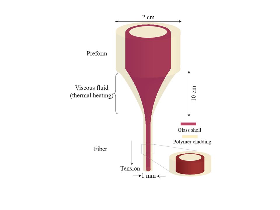
Figure 1: Optical-fiber thermal drawing. Preform is heated at elevated temperature to viscous fluid, and stretched into extended fibers by applied tension. This preform is specially designed with a thin cylindrical shell in polymer matrix.

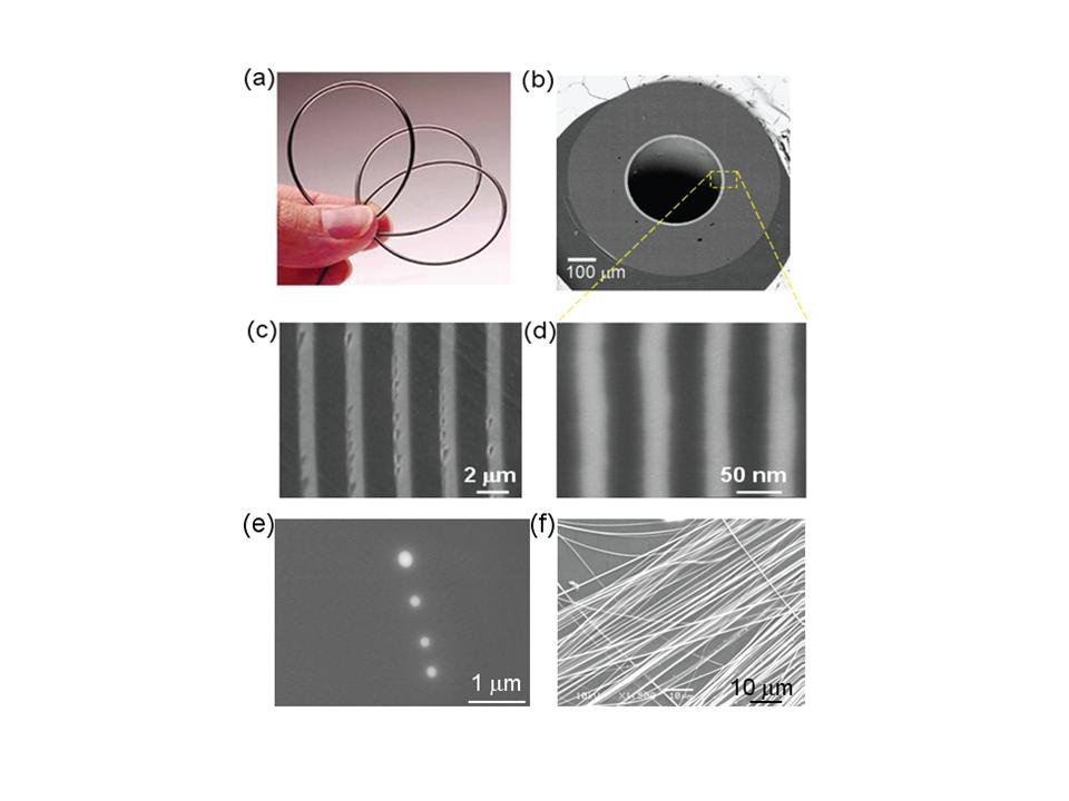
Figure 2: SEM micrographs of cylindrical shells in fiber. (a) Photograph of fiber. (b) SEM of fiber cross-section. Magnified view of multilayer structures reveals the thickness of micrometer (c) and tens of nanometers (d), respectively. Bright and dark color for glass and polymer in SEM, respectively. (e) showing layer breakup into circles in the fiber cross-section, while (f) presenting the continuous filaments obtained from fiber after dissolving polymer matrix.

Uniform layer thicknesses, down to micrometers or even to nanometers, have been successfully achieved in fibers by this method. Mechanically flexible fibers with a uniform diameter have been produced, as shown in Fig. 2(a). Fig. 2(b) shows a typical Scanning Electron Microscope (SEM) micrograph of a cross-section with $1$ $\mathrm{mm}$ fiber diameter. Magnified SEM micrographs in Fig. 2(c) and (d), for two different fibers, reveal high-quality multiple-layer structures with thicknesses on the order of micrometers and tens of nanometers, respectively.

Ideally, the cross-section of the resulting fibers retains the same structure and relative sizes of the components as in the preform. If the layer thickness becomes too small, however, we observed the layers to break up azimuthally, as shown in the cross-section of Fig. 2(e), while continuity along the axial direction remains intact. In this fashion, a thin cylindrical shell breaks into filament arrays embedded in a fiber Deng2008 ; Deng2009 . After dissolving the polymer cladding, the resulting separated glass filaments are shown in Fig. 2(f) Deng2008 .

As a first step towards understanding these observations, we will consider simplified geometries consisting of a thin cylindrical shell in the cladding matrix. The question, here, is whether the classical capillary instability from radial fluctuations is relevant to the attained thin uniform shells and the observed azimuthal breakup at further reduced thicknesses. Moreover, we want to know whether classical capillary instability can provide guidance for materials selections and fabrication processing in our microstructured fibers.

III Governing Equations

During thermal drawing, the temperature is set above the softening points of all the materials, which consequently are in the viscous fluid state to enable polymer and glass codrawing. To describe this fluid flow, we consider the incompressible Navier–Stokes (NS) equations Batchelor00 :

$$\begin{cases}\rho\left[\partial_{t}\vec{u}+\left(\vec{u}\cdot\nabla\right)\vec{u}\right]=-\nabla p+\nabla\cdot\left[\eta\frac{\nabla\vec{u}+\left(\nabla\vec{u}\right)^{T}}{2}\right]-\gamma\kappa\vec{n}\delta,\\ \nabla\cdot\vec{u}=0,\end{cases}$$ (1)

where $\vec{u}$ is velocity, $p$ is pressure, $\rho$ is materials density, $\eta$ is viscosity, $\gamma$ is interfacial tension between glass and polymer, $\delta$ is the delta function ($\delta=1$ at the polymer and glass interface and $\delta=0$ otherwise), $\kappa$ is curvature of interface, and $\vec{n}$ is a unit vector at interface.

To identify the operating regime of the fiber drawing process, we consider the relevant dimensionless numbers. The Reynolds number ($\mathrm{Re}$), Froude number ($\mathrm{Fr}$), and capillary number($\mathrm{Ca}$) are:

$$\mathrm{Re=\frac{\rho Uh}{\eta},Fr=\frac{U^{2}}{gh},Ca=\frac{\eta U}{\gamma},}$$ (2)

where $\rho\approx 10^{3}$ $\mathrm{kg/m^{3}}$ is the density of the materials, $g\approx 10$ $\mathrm{m/s^{2}}$ is gravity, $U\approx 5$ $\mathrm{mm/s}$ is drawing speed, $\eta\approx 10^{5}$ $\mathrm{Pa\cdot s}$ is viscosity, $h\approx 100$ $\mathrm{nm}$ is the layer thickness, and $\gamma=0.1$ $\mathrm{N/m}$ is surface tension between polymer and glass Hart2004 ; Hartthesis . Therefore, these dimensionless numbers in a typical fiber draw are $\mathrm{Re}\approx 10^{-10}$, $\mathrm{Fr}\approx 10^{2}$ and $\mathrm{Ca}\approx 10^{4}$. Small $\mathrm{Re}$ number, large $\mathrm{Fr}$ number, and large $\mathrm{Ca}$ number imply a weak inertia term, negligible gravity, and dominant viscosity effects, respectively. In addition, since the fiber diameter is $D\approx 1$$\mathrm{\mbox{}\mbox{}mm}$ and the length of the neck-down region is $L\approx 10$ $\mathrm{cm}$, the ratio $D/L\approx 1/100$ is much less than $1$, and thus the complicated profile of neck-down cone is simplified into a cylindrical shape for the purpose of easier analysis.

IV Simulation Algorithm

To develop a quantitative understanding of capillary instability in a cylindrical-shell geometry, direct numerical simulation is performed using the finite element method. In order to isolate the effect of radial fluctuations, we impose cylindrical symmetry, so the numerical simulation simplifies into a $\mathrm{2D}$ problem in the $(r,z)$ plane (where the $\nabla$ operations are replaced by their cylindrical forms). Although the low $\mathrm{Re}$ number means that one could accurately neglect the $(\vec{u}\cdot\nabla)\vec{u}$ nonlinear inertia term and solve only the time-dependent Stokes problem, we solve the full NS equations because of the convenience of using available software supporting these equations and also to retain the flexibility to consider large $\mathrm{Re}$ regimes in the future.

Our simulation algorithm is briefly presented in Fig. 3(a). The geometry of a cylindrical shell is defined by two interfaces $\mathrm{I}$ and $\mathrm{II}$ in Fig. 3(b). The flow field ($\vec{u},p$) is calculated from Navier–Stokes equations, as seen in Fig. 3(c). Consequently, this new flow field generates interface motion, resulting in an updated interface and an updated flow field. By these numerical iterations, the interface gradually evolves with time.

More specifically, the time-dependent interfaces $\mathrm{I}$ and $\mathrm{II}$ can be expressed as follows:

$$\begin{cases}r_{1}(z,t)=&r_{0}+\varepsilon_{1}(z,t),\\ r_{2}(z,t)=&2r_{0}+\varepsilon_{2}(z,t),\end{cases}$$ (3)

where $r_{0},2r_{0}$ are the unperturbed radii of interface $\mathrm{I}$ and $\mathrm{II}$, $\varepsilon_{1}(z,t),\varepsilon_{2}(z,t)$ denote the interfacial perturbations that grow with time.

The initial perturbations at interface $\mathrm{I}$ and $\mathrm{II}$ are given by cosine-wave shapes:

$$\begin{cases}\varepsilon_{1}(z,0)=&\varepsilon_{0}\mathrm{cos}(2\pi z/\lambda),\\ \varepsilon_{2}(z,0)=&2\varepsilon_{0}\mathrm{cos}(2\pi z/\lambda),\end{cases}$$ (4)

where $\varepsilon_{0},2\varepsilon_{0}$ are the perturbation amplitudes, and $\lambda$ is the initial perturbation wavelength.

Numerical challenges in the simulations arise from the nonlinearity, moving interfaces, interface singularities, and the complex curvature Eggers1997 ; Scardovelli1999 . A level-set function $\phi(\vec{x},t)$ is coupled with the NS equations to track the interface (see Appendix 1) Osher1988 ; Osher2001 ; Sethian2003 , where the interface is located at the $\phi=0.5$ contour and the $\phi$ evolution is given by $\vec{u}$ via:

$$\phi_{t}+\vec{u}\cdot\vec{\nabla}\phi=0.$$ (5)

The local curvature ($\kappa$) at an interface is given in terms of $\phi$ by:

$$\kappa=\nabla\cdot\vec{n}=\nabla\cdot\frac{\nabla\phi}{|\nabla\phi|}\\ =\frac{(\phi_{r}^{2}\phi_{zz}+\phi_{z}^{2}\phi_{rr})+(\phi_{r}^{2}+\phi_{z}^{2})\phi_{r}/r-\phi_{r}\phi_{z}(\phi_{rz}+\phi_{zr})}{(\phi_{r}^{2}+\phi_{z}^{2})^{3/2}}.$$ (6)

For numerical stability reasons, we add an artificial diffusion term proportional to a small parameter $D$ in Eq. 5 (see Appendix 4); the convergence as $D\rightarrow 0$ is discussed in the next section.

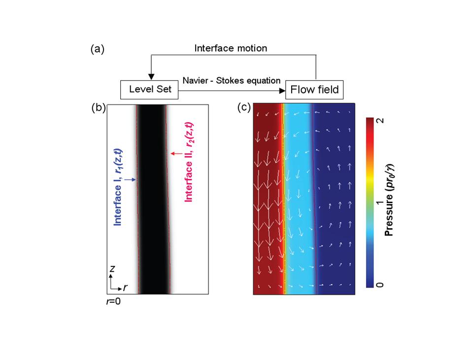
Figure 3: Simulation algorithm. (a) Schematic of algorithm. (b) Interfaces $\mathrm{I}$ and $\mathrm{II}$ of cylindrical shell are defined by a level set function. (c) Flow field is determined by the NS equations (color scale for pressure and arrows for fluid velocity).

V Simulation Results

In the low $\mathrm{Re}$ regime, the NS equations are linear with respect to the flow velocity $\vec{u}$ because the inertia term $(\vec{u}\cdot\nabla)\vec{u}$ is negligible, but they are not linear with respect to the geometry of the interface shape except in the limit of small perturbations. A linear theory for small geometric perturbations was formulated for the cylinder by Tomotika Tomotika1935 and for a cylindrical shell with a cladding of equal viscosity by Stone and Brenner Stone1996 . Our full simulation should, of course, reproduce the results of the linear theory for small perturbations, but also allows us to investigate larger perturbations beyond the regime of the linear theory, and we can also consider the more general case of a cylindrical shell with a cladding of unequal viscosity.

V.1 Numerical convergence

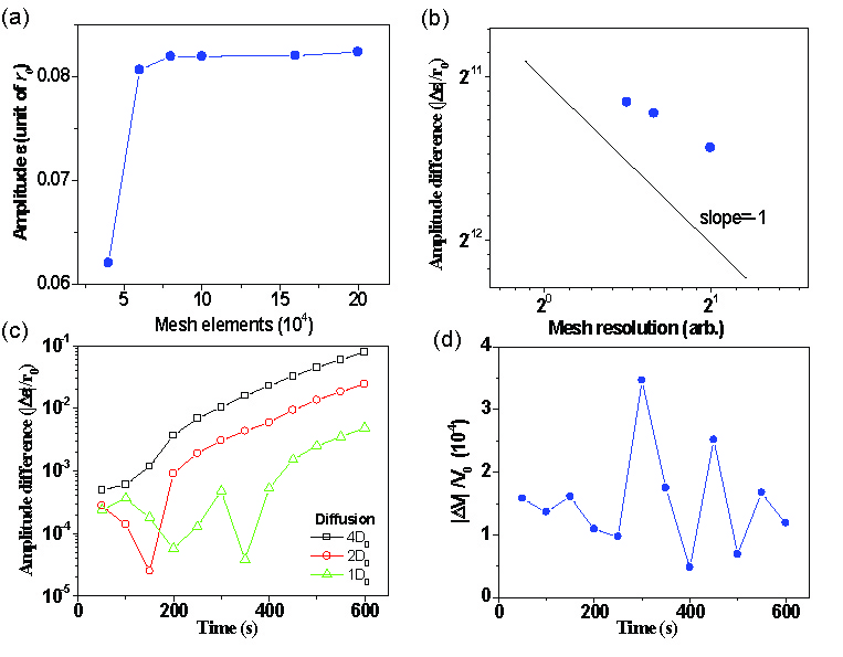
Figure 4: Numerical convergence with respect to various approximations in the simulation. (a) Numerical convergence shown by instability amplitude at time t=300 seocnds vs number of mesh elements; (b) established errors ($|\Delta\varepsilon|$ corresponding to higher resolution) versus resolution (solid line=expected asymptotic rate); (c) the artificial diffusion term for numerical stability, and (d) the numerical errors represented by deviations from volume conservation.

In order to establish the accuracy of the simulation, we first investigated the convergence with respect to the various approximations: the time integration tolerance ($\rightarrow 0$), the mesh resolution ($\rightarrow\infty$), and an artificial diffusion term $\mathbf{\mathrm{D}}$ ($\rightarrow 0$). The time integration is performed by a fifth-order backward differentiation formula, characterized by specified relative and absolute error tolerances ($\mathrm{err_{rel}}=10^{-4}$ and $\mathrm{err_{abs}=10^{-5}}$) with acceptable accuracy ($\approx 10^{-3}$). Fig. 4(a) shows numerical convergence of the instabiltiy amplitude $\min_{z}\varepsilon_{1}(z,t)$ at time t=300 seocnds as a fucntion of the number of triangular mesh elements. From last four data points in (a), the convergence of $|\Delta\varepsilon|/r_{0}$ with respect to the mesh resolution, compared with a very fine mesh of $20\cdot 10^{4}$ mesh elements, is presented in Fig. 4(b). Because of the PDE’s discontinuous coefficient, we expect 1st-order convergence: that is error $\sim$ 1/(mesh resolution), corresponding to slope $-1$ (solid line) in Fig. 4(b): the data points appear to be approaching this slope, but we are not able to measure errors at high enough resolution to verify the convergence rate conclusively. However, we found $10\cdot 10^{4}$ mesh elements, corresponding to a typical element diameter $\approx 0.01r_{0}$ , yield good accuracy ($\approx 10^{-3}$ error). The physical results are recovered in the limit $D\rightarrow 0$, and so we must establish the convergence of the results as $D$ is reduced and identify a $D$ small enough to yield accurate results while still maintaining stability. Fig. 4(c) demonstrates this convergence in the simulation by calculating the amplitude difference $|\Delta\varepsilon|/r_{0}$ compared with $D=0.5D_{0}$ ($D_{0}=10^{-14}\mathrm{m^{2}/s}$ in Appendix 1), and 3 digits of accuracy are attained by $D=D_{0}$. Accordingly, the numerical parameters throughout the following simulations are $err_{rel}=10^{-4},err_{abs}=10^{-5},D=1.0D_{0}$, and $10\cdot 10^{4}$ mesh elements. As an additional check, the volume of the incompressible fluid shell between the two interfaces should be conserved. As shown in Fig. 4(d), the numerical errors in the simulation leads to only a small volume deviation, ($|V(t)-V(0)|/V(0)=|\Delta V(t)|/V(0)$), of less than $0.4\%$. We conclude that the finite-element level-set approach is numerically reliable for the simulation of capillary instabilities.

V.2 Instability evolution

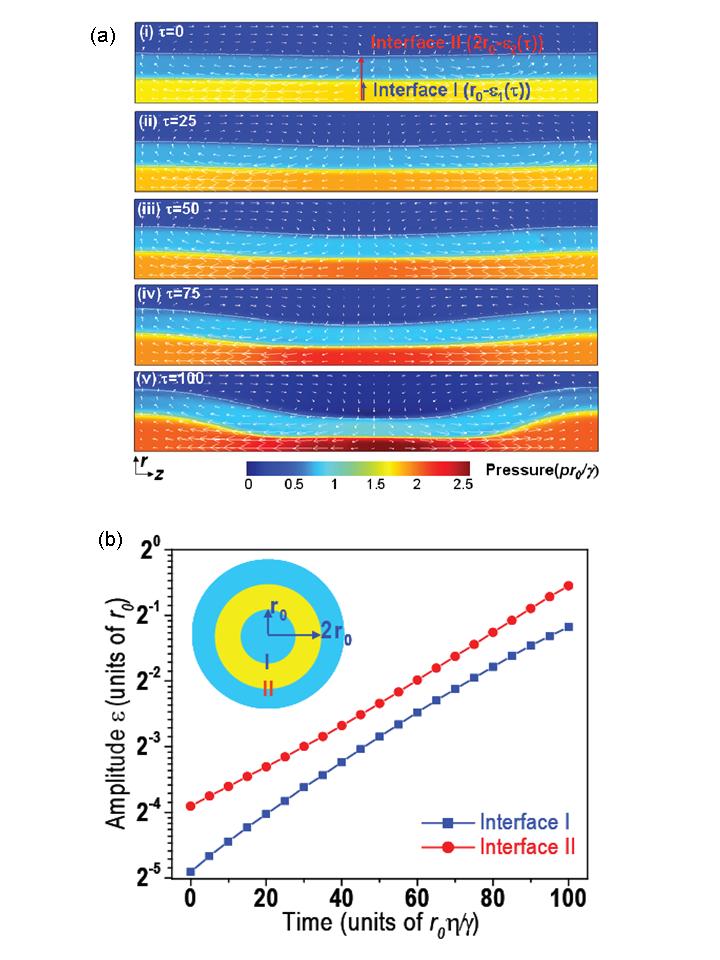
Figure 5: (a) Snapshot of the flow field and interfaces during instability evolution. Color scale for pressure, arrows for fluid velocity. (b) The instability amplitude grows exponentially with time at interfaces $\mathrm{I}$ and $\mathrm{II}$.

The evolution of a capillary instability can be obtained from direct numerical simulation. Fig. 5(a) (i)–(v) presents snapshots of the flow field and interface. (i) Initially, the pressure of the inner fluid is higher than that of the outer fluid due to Laplace pressure ($p=\gamma\kappa$) originating from azimuthal curvature of the cylindrical geometry at interfaces $\mathrm{I}$ and $\mathrm{II}$. (ii)–(iv) The interfacial perturbations generate an axial pressure gradient $\Delta p$, and hence a fluid flow occurs that moves from a smaller-radius to a larger-radius region for the inner fluid. Gradually the amplitude of the perturbation is amplified. (v) The shrunk smaller-radius and expanded larger-radius regions of inner fluid further enhance the axial pressure gradient $\Delta p$, resulting in a larger amplitude of the perturbation. As a result, the small perturbation is exponentially amplified by the axial pressure gradient.

Fig. 5(b) shows the instability amplitude $\min_{z}\varepsilon(z,t)$ at interfaces $\mathrm{I}$ and $\mathrm{II}$ growing with time exponentially on a semilog scale in the plot. The instability time scale in the simulation is about $372\pm 3$ $\mathrm{sec}$ by fitting the curve to an exponential $\varepsilon\sim e^{t/\tau}$. Linear theory predicts time scale of $\tau\approx 334$ $\mathrm{sec}$ Stone1996 (see Appendix 2). Thus, simulation is consistent with the linear theory, in terms of the instability time scale.

V.3 Beyond the linear theory

More quantitatively, for small perturbations or short times, exponential growth of the perturbation amplitude is expected from the linear theory. However, at later times, when the perturbation has grown sufficiently, one expects the linear theory to break down. We observe significant deviations from the linear theory if the amplitude is above $10\%$ of the cylinder radius $r$ (corresponding to time $40r\eta/\gamma$), as shown in Fig. 6 (taking interface $\mathrm{I}$ as an example). For example, at perturbation amplitudes of around $25\%$ of $r$ (time $70r\eta/\gamma$), the deviations of the simulation data from the linear theory is almost $20\%$ .

The length scaling of the instability is studied as well. After rescaling time and distance by the same factor (so that the initial radius is scaled by $0.25,0.5,1,2$, and $4$), all the data collapse onto a single master curve, as shown in Fig. 6. This length scaling originates from the low $\mathrm{Re}$ regime, which implies that the NS equations are approximately linear with respect to $\vec{u}$; this gives rise to the well known scale invariance in the Stokes regime Batchelor00 .

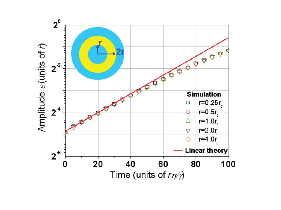
Figure 6: Growth of perturbation amplitude as a function of time. At small amplitudes below $10\%$ $r$, the perturbation grows exponentially as expected from linear theory. At large amplitude above $10\%$ $r$, significant deviations from linear theory occur. Scale invariance, with various values of r superimposed, is expected in the Stokes regime with low Re number.

V.4 Unequal viscosities

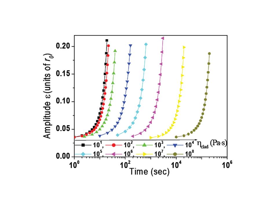
Figure 7: Time-dependent perturbation amplitude curves for various cladding viscosities ($\eta_{\mathrm{clad}}$), but with a fixed shell viscosity ($\eta_{\mathrm{shell}}=10^{5}\mathrm{Pa\cdot s}$).

We now investigate the dependence of instability timescale on cladding viscosity ($\eta_{\mathrm{clad}}$) with a fixed shell viscosity ($\eta_{\mathrm{shell}}$), in order to help us to identify suitable cladding materials for fiber fabrication. As viscosity slows down fluid motion, the low-viscosity cladding has a faster instability growth rate and a shorter time scale, while the high-viscosity cladding has a slower instability growth rate and a longer instability time scale. Fig. 7 shows the time-dependent perturbation amplitude curves for various viscosity contrast $\eta_{\mathrm{clad}}/\eta_{\mathrm{shell}}$ by changing the cladding viscosity ($\eta_{\mathrm{shell}}=10^{5}$ $\mathrm{Pa\cdot s}$). Instability time scale for the each given viscosity contrast is obtained by exponentially fitting the curves in Fig. 7. Instability time scale ($\tau$) as a function of viscosity contrast is presented in Fig. 8.

The existing linear theory has only been solved in case of equal viscosity, and predicts that the instability time scale is proportional to the viscosity $\tau\sim\eta$ Stone1996 . We obtain a more general picture of the instability time scale for unequal viscosity by considering two limits. In the limit of negligible cladding viscosity, $\eta_{\mathrm{clad}}\rightarrow 0$, the instability time scale should be determined by $\mathrm{\mathrm{\eta}}_{\mathrm{shell}}$, and from dimensional analysis should be proportional to $r\eta_{\mathrm{shell}}/\gamma$ , assuming that the inner and outer radius are comparable and so we take $r$ to be the average radius. In the opposite limit of $\eta_{\mathrm{clad}}\rightarrow\infty$ , the time scale should be determined by $\eta_{\mathrm{clad}}$ and hence should be proportional to $r\eta_{\mathrm{clad}}/\gamma$. In between these two limits, we expect the time scale to smoothly interpolate between the $r\eta_{\mathrm{shell}}/\gamma$ and $r\eta_{\mathrm{clad}}/\gamma$ scales. Precisely this behavior is observed in our numerical calculations, as shown in Fig. 8.

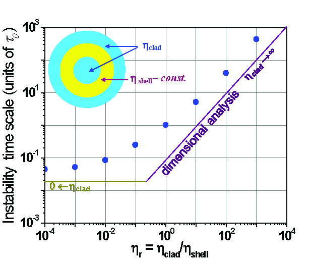
Figure 8: An instability time scale ($\tau$) for unequal viscosity with a fixed shell viscosity ($\eta_{\mathrm{shell}}$). In the limit of $\eta_{\mathrm{clad}}\rightarrow 0$, $\tau$ is determined by $\eta_{\mathrm{shell}}$ and approaches to a constant. In the opposite limit of $\eta_{\mathrm{clad}}\rightarrow\infty$, $\tau$ should be determined by $\eta_{\mathrm{clad}}$ and is linearly proportional to $\eta_{\mathrm{clad}}$. Between these two limits of $\eta_{\mathrm{clad}}$, $\tau$ smoothly interpolates between the corresponding time scales.

VI Estimate of radial instability timescale

In the previous section, we surveyed the capillary instability of a concentric-cylindrical shell by numerical simulations. We proceed to apply these results to investigate the instability time scale dependent on various physical parameters including geometry (e.g., radius and shell thickness) and materials properties (viscosity) in a broad range, exploiting the accuracy of simple dimensional analysis demonstrated in the previous section and providing guidance of our fiber drawing.

The calculated instability time scale ($\tau$) for different values of the radius ($r$) and the viscosity ($\eta$) is displayed in Fig. 9. The cross-sectional geometry in the calculation is shown in the inset: interface $\mathrm{I}$ is located at radius $r$, the cylindrical-shell thickness is $h$, and interface $\mathrm{II}$ is at radius $R=r+h$. The interfacial tension in the calculations was set to $\gamma=0.1\mbox{}\mathrm{N/m}$, which was the measured interfacial tension between thermoplastic polymer and chalcogenide glass used in our microstructured fibers Hart2004 .

Two cases are considered: one is equal viscosity $(\eta_{\mathrm{shell}}=\eta_{\mathrm{clad}})$, and the other is unequal viscosity $(\eta_{\mathrm{shell}}\neq\eta_{\mathrm{clad}})$. In the case of $\eta_{\mathrm{shell}}=\eta_{\mathrm{clad}}$, the instability time scale is calculated exactly from Stone and Brenner’s linear theory Stone1996 ,

$$\tau=\frac{\eta r}{\gamma\max_{\lambda}\Psi(\lambda,R/r)},$$ (7)

where the fastest growth factor $\mathrm{\max_{\lambda}}\Psi(\lambda,R/r)$ was found by searching numerically within a wide range of wavelengths $\lambda$ for a certain value of $R/r$ (Eq. 23 in Appendix 2). Fig. 9 plots this time scale versus radius for $\mathrm{\eta=10^{5}\mbox{}\mbox{}Pa\cdot s}$ corresponding to As₂Se₃–PES, compared to the dwelling time $\tau_{\mathrm{dwelling}}\approx 100$ $\mathrm{sec}$ which is defined by the time of materials in viscous state before exiting hot furnace to be frozen in fiber during thermal drawing Hartthesis .

In the other case of $\eta_{\mathrm{shell}}\neq\eta_{\mathrm{clad}}$ (in the $\eta_{\mathrm{clad}}/\eta_{\mathrm{shell}}\gg 1$ regime as discussed in Section V.4), the instability time scale can be roughly estimated from dimensional analysis. Although dimensionless analysis does not give the constant factor, for specificity, we choose the constant coefficient from the Tomotika model Tomotika1935 ,

$$\tau\approx\frac{2r\eta_{clad}}{\gamma\max_{\lambda}\left[(1-x^{2})\Phi(x,\eta_{clad}/\eta_{shell})\right]},$$ (8)

where the fastest growth factor $\mathrm{\max_{\lambda}[}(1-x^{2})\Phi(x,\eta_{clad}/\eta_{shell})]$ was found numerically by searching a wide range of wavelengths ($x=2\pi r/\lambda$) [$\mathrm{\Phi(x,\eta_{clad}/\eta_{shell})}$ is a complicated implicit function of wavelength and viscosity contrast given in Ref. Tomotika1935 ]. Fig. 9 plots the time scale for $\eta_{\mathrm{shell}}=10$ $\mathrm{Pa\cdot s}$, $\mathrm{\mathrm{\eta}_{clad}=10^{5}}$ $\mathrm{Pa\cdot s}$, corresponding to Se–PSU showing that the observed stability of shells of radius $\mathrm{\approx 250\mbox{}\mu m}$ is consistent with the radial stability criterion ($\mathrm{\tau>\tau_{dwelling}}$). On the other hand, if $\mathrm{\eta_{clad}}$ is reduced to $\mathrm{10^{3}}$ $\mathrm{Pa\cdot s}$ with the same shell materials, corresponding to Se–PE, we predict that radial fluctuations alone will render the shell unstable for any radius $r\leq 1$ $\mathrm{mm}$.

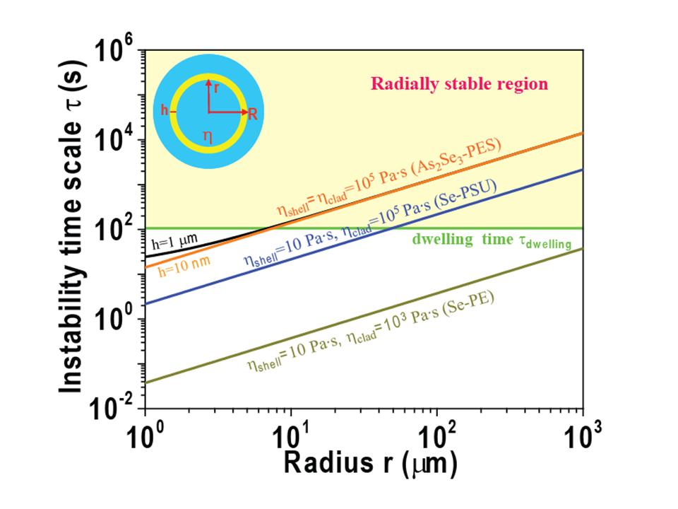
Figure 9: Radial stability map. Linear theory calculations of the instability time scale ($\tau$), which is dependent on the radius, thickness, and viscosity. Inset shows cross-sectional geometry of cylindrical shell. In our experiments, the dwelling time of thermal drawing is around $\tau_{\mathrm{dwelling}}\approx 100$ $\mathrm{sec}$, and the fiber radius $r\approx 500$ $\mathrm{\mathrm{\mu m}}$. Radially stable region is shaded yellow for $\tau>\tau_{\mathrm{dwelling}}$, while the unstable region corresponds to $\tau<\tau_{\mathrm{dwelling}}$.

VII Applications in Microstructured Fibers

In this section, we consider in more detail the application of these analyses to understand observed experimental results, and in particular the observed stability (or instability) of thin shells and filaments. We examine whether our stability analysis can provide guidance in materials selection and in the the understanding of attainable feature sizes. Because we only considered radial fluctuations, our analysis provides a necessary but not sufficient criterion for stability. Therefore, the relevant questions are whether the criterion is consistent with observed stable structures, whether it is sufficient to explain the observed azimuthal breakup, and what materials combinations are excluded. Below, in Sec VII.1 we consider the application of radial stability analysis to the observed stability or instability of cylindrical shells. In Sec VII.2 we look at the impact on materials selections. Finally, in Sec VII.3, we show that the observed stability of the resulting nanoscale filaments is consistent with the Tomotika model.

VII.1 Comparison with observations for cylindrical shells

The radial stability map of Fig. 9 is consistent with the experimental observations (the default cylindrical shell radius $\approx 250$$\mathrm{\mu m}$). First, the map predicts that feature sizes down to submicrometers and hundreds of nanometers are consistent with radial stability for the equal-viscosity materials combination of $\eta_{\mathrm{clad}}=\eta_{\mathrm{shell}}=10^{5}$ $\mathrm{Pa\cdot s}$, which corresponds to As₂Se₃–PES or As₂S₃–PEI. For As₂Se₃–PES, Fig.2 (c) shows that a shell thickness of As₂S₃ of $1$ $\mathrm{\mathrm{\mu m}}$ is obtained; in other work, layers of As₂S₃ down to $15$ $\mathrm{nm}$ have been achieved as well Deng2008 . For As₂S₃–PEI, Fig.2 (d) demonstrates a thickness of $\mathrm{As_{2}S_{3}}$ down to 32 $\mathrm{nm}$. Second, the map is consistent with thicknesses down to submicrometers for unequal-viscosity materials with $\eta_{\mathrm{clad}}=10^{5}$ $\mathrm{Pa\cdot s}$, $\eta_{\mathrm{shell}}=10$ $\mathrm{Pa\cdot s}$, which corresponds to Se–PSU. Se layers with thickness on the order of $1$ $\mathrm{\mathrm{\mu m}}$ have been demonstrated in Se–PSU fiber Deng2008 .

The radial stability map, nevertheless, is not sufficient to explain the azimuthal instability at further reduced thicknesses down to tens of nanometers. The stability map of Fig. 9 predicts that a $\mathrm{Se}$ layer in a Se–PSU combination should be radially stable down to tens of nanometers. However, we found in experiments [Fig. 2(e, f)] that a Se shell with thickness $<100$ nm breaks up into continuous filament arrays Deng2008 ; Deng2009 , which means that the mechanism for this breakup is distinct from that of purely radial fluctuations. For another As₂Se₃–PES materials combination, this filamentation of As₂Se₃ film was also observed as the thickness is reduced down to $10$ $\mathrm{nm}$ Deng2008 . Future work will elucidate this filamentation mechanism by performing $\mathrm{3D}$ numerical simulation to explore the azimuthal fluctuations.

VII.2 Materials selection

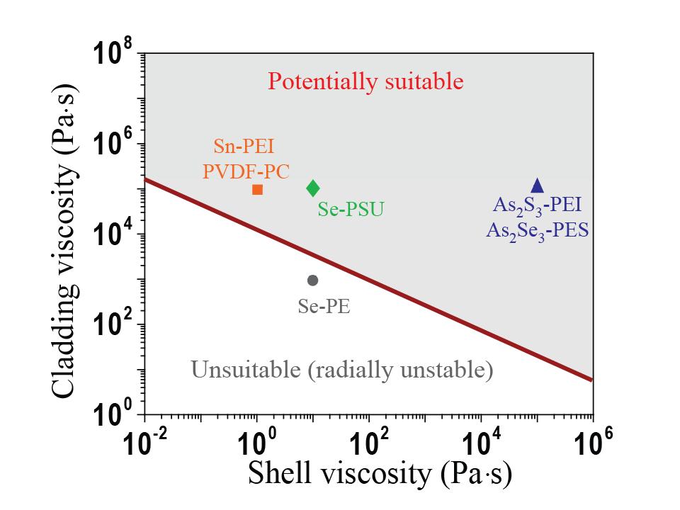
Figure 10: Calculated shell–cladding viscous materials selection map during thermal drawing ($\tau_{\mathrm{dwelling}}=100$ sec). A red line for instability time for dwelling time $\tau=\tau_{\mathrm{dwelling}}$. The shaded region above the red line indicates potentially suitable viscous materials combination ($\tau>\tau_{\mathrm{dwelling}}$), those in which radial instabilities alone do not cause breakup. The region below the red line indicates radially unstable materials combinations ($\tau<\tau_{\mathrm{dwelling}}$), such as $\mathrm{Se-PE}$ materials combination, which are unstable for thermal drawing.

Given the viscosities and surface tension of a particular material pair, we can use Fig. 9 to help determine whether that pair is suitable for drawing: if it is radially unstable, then it is almost certainly unsuitable (unless the process is altered to somehow compensate), whereas if it is radially stable then the pair is at least potentially suitable (if there are no other instabilities). Viscosities of materials used in fiber drawing are obtained as follows: the viscosities of semiconductor glasses (Se, As₂Se₃, As₂S₃) are calculated from an empirical Arrhenius formula at the associated temperature during thermal drawing (more details in Appendix 3); several thermoplastic polymers (PSU, PES, and PEI) have similar viscosities $\eta_{\mathrm{polymer}}\approx 10^{5}$ $\mathrm{Pa\cdot s}$ during fiber drawing Hartthesis ; and the viscosity of the polymer PE is $10^{3}$ $\mathrm{Pa\cdot s}$ at temperature $\mathrm{T=250^{\circ}C}$ Dobrescu83 . The polymer–glass surface tension is typically $\gamma=0.1$ N/m Hart2004 for all of these materials. Assuming a cylindrical shell of radius $\approx 250$ $\mathrm{\mu m}$ and a dwelling time of thermal drawing $\approx 100$ $\mathrm{sec}$, we can classify each materials combination by whether it falls in the $\tau>\tau_{\mathrm{dwelling}}$ yellow region (radially stable) of Fig. 9 or in the $\tau<\tau_{\mathrm{dwelling}}$ white region (radially unstable).

These materials combinations are presented in Fig. 10. The boundary line in red, which indicates the viscous combinations that satisfy $\tau=\tau_{\mathrm{dwelling}}$, divides the map into two areas. The shaded area above the boundary line is the region of potentially suitable materials combinations for fiber drawing (As₂Se₃–PES, As₂S₃–PEI, Se–PSU) Abouraddy2007 ; Deng2008 ; while the materials combinations below the boundary line are unsuitable due to radial instability. Here, the only materials combination which seems to be definitely excluded in this regime due to radial instability is Se–PE. The polymer–polymer materials combination of PVDF–PC (polyvinylidene fluoride, PVDF, a piezoelectric polymer; polycarbonate, PC) is potentially suitable for thermal drawing, and this possibility has been confirmed by recent experiments Egusa . Moreover, since a high viscosity cladding improves stability (increase $\tau$), we predict that a wider variety of shell materials with low viscosity may possibly be employed in microstructured fibers, such as the metals $\mathrm{Sn}$ and $\mathrm{\mathrm{I}n}$ Abouraddy2007 ; Culpin1957 . These various available classes of metals, polymers and semiconductors expand the potential functionalities of devices in microstructured fibers.

VII.3 Stability of continuous filaments down to submicrometer/nanometer scale

As shown in Fig. 2(e–f), in some cases the initial shell breaks up (azimuthally) into long cylindrical filaments Deng2008 ; Deng2009 . These filaments themselves should be subject to the classic capillary instability and in principle should eventually break up into droplets. In our fiber-drawing experiments, however, no further instability is observed: the filaments are observed to remain continuous and unbroken over at least cm length scales with diameters reaching submicrometer scales Deng2008 ; Deng2009 . Since a cylindrical filament of one fluid surrounded by another should be described exactly by the Tomotika model, it is important to know whether the observed stability is consistent with this model, or otherwise requires some additional physical mechanism (such as visco-elasticity) to explain. In this section, we find that the timescale of instability predicted by the Tomotika model exceeds the dwelling time of fiber drawing, making it unsurprising that filament instability is not observed. In fact, we show that the instability time scale exceeds the dwelling time even under unrealistically conservative assumptions: that the filaments appear immediately in the fiber drawing, that the maximum instability growth rate is cumulative even though the lengthscale achieving maximum growth changes with the filament radius during drawing, and that the polymer viscosity is always at its minimum value (corresponding to the highest temperature point).

An instability with time scale $\tau$ corresponds to exponential growth of a fluctuation amplitude $\epsilon$ according to $\frac{d\epsilon}{dt}=\epsilon/\tau$. If $\tau$ is time varying, then the total amplitude growth is $\mathrm{exp}[\int dt/\tau(t)]$. Converting to $dz=v(z)dt$ for a position-dependent axial flow velocity $v(z)$ during thermal drawing, we therefore obtain a total exponential growth factor:

$$\Gamma=\int_{0}^{L}\frac{dz}{v(z)\tau(z)},$$ (9)

where $z\in[0,L]$ is axial position in the neck-down region with length $(\mathrm{L=6\mbox{ $$}}\mathrm{cm})$. $\Gamma\gg 1$ corresponds to breakup, while $\Gamma\ll 1$ corresponds to stability.

In order to provide a conservative estimation of filament stability, the capillary instability time is calculated from the fastest growth factor at each axial location (this is a very conservative estimate), and the polymer viscosity is set to be the minimum value (at the highest temperature) during thermal drawing. The capillary instability time scale is calculated based on the Tomotika model as follows Tomotika1935 ,

$$\tau(z)=\frac{2r\eta_{\mathrm{polymer}}(z,T)}{\gamma\left\{\max_{\lambda}\left(1-x^{2}\right)\Phi\left[x,\eta_{\mathrm{polymer}}(z,t)/\eta_{\mathrm{clad}}(z,t)\right]\right\}}.$$ (10)

The complex shape of neck-down profile is fitted from experiment can be approximately described by following formula,

$$\frac{R(z)}{R(0)}=(1+k\frac{z}{L})^{-1/p},\quad k=\left[\frac{R(0)}{R(L)}\right]^{p}-1,\quad p=2.$$ (11)

Due to the incompressibility of the viscous fluid, the velocity of flow scales inversely with area:

$$\frac{v(z)}{v(0)}=\frac{R^{2}(0)}{R^{2}(z)},$$ (12)

where $\mathrm{v(0)=4\times 10^{-3}\mbox{}mm/sec}$ is the preform velocity. Again by incompressibility, the filament radius $(\mathrm{r})$ should scale as the fiber radius $(R)$:

$$\frac{r(z)}{r(0)}=\frac{R(z)}{R(0)}.$$ (13)

The temperature distribution during thermal drawing, fit from experiment, is found to be approximately parabolic,

$$T=T_{\mathrm{max}}-\left(T_{\mathrm{max}}-T_{\mathrm{min}}\right)\left(2\frac{z}{L}-1\right)^{2}.$$ (14)

In calculations, parameters for the typical $\mathrm{As_{2}Se_{3}}$–PES fiber drawing are $\mathrm{R(0)=1}$ cm, $\mathrm{s=20}$, $\mathrm{L=6}$ cm, $\mathrm{p=2}$, $\mathrm{T_{max}=260}\,{}^{\circ}$C, $\mathrm{T_{min}=210}\,{}^{\circ}$C, $\mathrm{r(L)=200}$ nm, $\mathrm{\eta_{polymer}=10^{6}}$ Pa$\cdot$s. Fig. 11 (b)–(d) presents the corresponding position–dependent variables including radius, velocity, temperature and viscosity. Finally, we obtain

$$\Gamma=0.90.$$ (15)

This satisfies $\Gamma<1$, but only barely—if this were an accurate estimate of the growth factor, instability might still be observed. However, the assumptions we made above were so conservative that the true growth factor must be much less than this, indicating the instability should not be observable during the dwelling time of fiber drawing. So, the observed filaments are consistent with the Tomotika model, although of course we cannot yet exclude the possibility that there are also additional effects (e.g., elasticity) that further enhance stability.

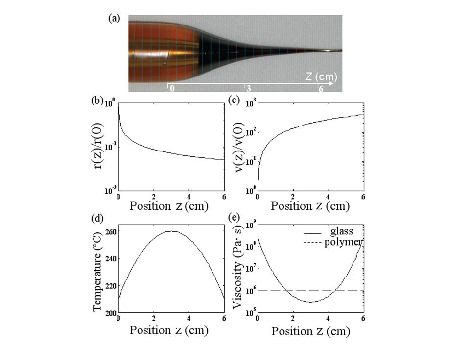
Figure 11: Relevant parameters in the neck-down region during thermal drawing. (a) Photograph of neck-down region from preform to fiber, (b)–(e) for the calculated radius, velocity, temperature and viscosity.

VII.4 Favorability of azimuthal versus axial instability

In experiments, we observed that thin films preferentially break up along the azimuthal direction rather than the axial direction. The discussion of the previous Section VII.3 suggests a simple geometrical explanation for such a preference, regardless of the details of the breakup mechanism. The key point is that any instability will have some characteristic wavelength $\lambda$ of maximum growth rate for small perturbations, and this $\lambda$ must be proportional to the characteristic feature size of the system, in this case the film thickness $d$. As the fiber is drawn, however, the thickness $d$ and hence $\lambda$ decreases. Now, we consider what happens to an unstable perturbation that begins to grow at some wavelength $\lambda_{0}$ when the thickness is $d_{0}$. If this is a perturbation along the axial direction, then the fiber-draw process will stretch this perturbation to a longer wavelength, that will no longer correspond to the maximum-growth $\lambda$ (which is shrinking), and hence the growth will be damped. That is, the axial stretching competes with the layer shrinking, and will tend to suppress any axial breakup process. In contrast, if $\lambda_{0}$ is an azimuthal perturbation, the draw-down process will shrink $\lambda_{0}$ along with the fiber cross-section at exactly the same rate that $d$ and $\lambda$ shrink. Therefore, azimuthal instabilities are not suppressed by the draw process. This simple geometrical argument immediately predicts that the first observed instabilities will be azimuthal (although axial instabilities may still occur if the draw is sufficiently slow).

VIII Concluding remarks

In this paper, motivated by recent development in microstructured optical fibers, we have explored capillary instability due to radial fluctuations in a new geometry of concentric cylindrical shell by 2D numerical simulation, and applied its theoretical guidance to feature size and materials selections in the microstructured fibers during thermal drawing processes. Our results suggest several directions for future work. First, it would be desirable to extend the analytical theory of capillary instability in shells, which is currently available for equal viscosity only, to the more general case of unequal viscosities — we have developed a very general theory in an appearing paper Liang2010 . Second, we plan to extend our computation simulations to include 3D azimuthal fluctuations together with radial fluctuations; as argued in Section VII.4, we anticipate a general geometrical preference for azimuthal breakup over axial breakup once the draw process is included. Third, there are many additional possible experiments that would be interesting to explore different aspects of these phenomena in more detail, such as employing different geometries (e.g., non-cylindrical), temperature-time profiles, or materials (e.g., Sn–PEI or Se–PE). Finally, by drawing more slowly so that axial breakup occurs, we expect that experiments should be able to obtain more diverse structures (e.g. axial breakup into rings or complete breakup into droplets) that we hope to observe in the future.

Appendix

1. Direct numerical simulation of concentric cylindrical shells

In the simulation, the level set function is defined by a smoothed step function reinitialized at each time step Olsson2005 ,

$$\phi(z,t)=\begin{cases}0&r<r_{1}(z,t)-\Lambda,\enskip r>r_{2}(z,t)+\Lambda\\ 1&r_{1}(z,t)+\Lambda<r<r_{2}(z,t)-\Lambda\\ 0.5&\mbox{otherwise}\end{cases},$$ (16)

where $r_{1}(z,t)$ and $r_{2}(z,t)$ are the radius of interfaces I and II of the coaxial cylinder, and $\Lambda$ is the half thickness of the discretized interface. The level set $\phi=1$, 0, and $0.5$ corresponds to the region of concentric cylindrical shell, of surrounding fluid, and interface, respectively. Contour $\Pi=\{X|\phi(X,t)=0.5\}$ tracks the interface $\mathrm{I}$ and $\mathrm{II}$.

A smoothed delta function is defined to project surface tension at interface,

$$\delta = 4\phi(1-\phi)=\begin{cases}1&|r-r_{1,2}|<\Lambda\\ 0&\mbox{otherwise}\end{cases}.$$

A smoothed step function is introduced to create a smooth transition of the level-set function $\phi$ from $0$ to $1$ across the interface,

$$\phi=\left[1+e^{(r-r_{1})/\Lambda}\right]^{-1}-\left[1+e^{(r-r_{2})/\Lambda}\right]^{-1}.$$ (17)

The boundary condition for the level set equation at the edge of the computational cell is

$$\vec{n}\cdot(-c\nabla\phi+\phi\vec{u})=0,$$ (18)

where $\vec{n}$ and $\vec{t}$ are the normal and tangential vectors at the boundary. In addition, boundary conditions for the NS equations are

$$\begin{cases}\vec{n}\cdot\vec{u}&=0,\\ \vec{t}\cdot\eta\left[\nabla\vec{u}+(\nabla\vec{u})^{T}\right]\vec{n}&=0.\end{cases}$$ (19)

In the simulation, time-stepping accuracy is controlled by an absolute and relative error tolerance ($\mathrm{err_{abs}}$ and $\mathrm{err_{rel}}$) for each integration step. Let $U$ be the solution vector at a given time step, $E$ be the solver’s estimated local error in $U$ during this time step, and $N$ be the number of degrees of freedom in the simulation. Then a time step is accepted if the following condition is satisfied,

$$\left[\frac{1}{N}\underset{i}{\sum}\left(\frac{|E_{i}|}{err_{abs}+err_{rel}|U_{i}|}\right)^{2}\right]^{{}^{1/2}}<1.$$ (20)

A triangular finite-element mesh is generated, and second-order quadratic basis functions are used in the simulation. Parameters for Fig. 5 in the simulation are $\rho=10^{3}$ $\mathrm{kg/m^{3}}$, $\eta=10^{5}$ $\mathrm{Pa\cdot s}$, $\gamma=0.6$ $\mathrm{N/m}$, $R=120$ $\mathrm{\mu m}$, $\mathrm{err_{rel}}=10^{-4},\mathrm{\mbox{}err_{abs}}=10^{-5},$ $D=D_{0}=10^{-14}$ $\mathrm{m^{2}/s}$.

2. Linear theory of concentric cylindrical shells with equal viscosities

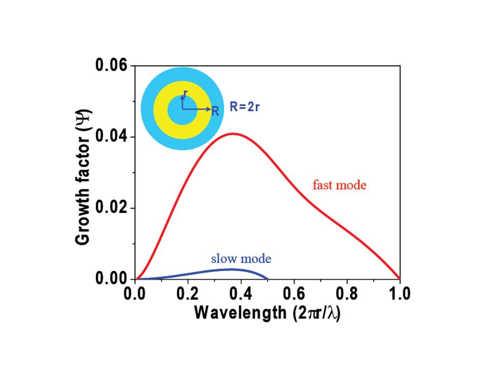
Figure 12: Growth factor of instability as a function of perturbation wavelength. Fast- and slow- modes occur at wavelengths above their respective critical wavelengths $\lambda_{f},\lambda_{s}$. Inset is a sketch of coaxial cylinder with radius $R=2r$ and equal viscosities.

A linear theory of capillary instability for a co-axial cylinder with equal viscosities is provided in the literature by Stone and Brenner Stone1996 . The growth rate ($\sigma$) for a wave vector $k=2\pi/\lambda$ is a solution of the following quadratic equations,

$$\left\{\sigma-\frac{k^{2}\gamma_{1}}{r\eta}\left[1-(rk)^{2}\right]\Lambda(r,r)\right\}\\ \times\left\{\sigma-\frac{k^{2}\gamma_{2}}{R\eta}\left[1-(Rk)^{2}\right]\Lambda(R,R)\right\}\\ =\frac{k^{4}\gamma_{1}\gamma_{2}}{rR\eta^{2}}\left[1-(rk)^{2}\right]\left[1-(Rk)^{2}\right]\Lambda(r,R)^{2},$$ (21)

where $r$ and $R$ are the radii of the unperturbed interfaces I and II, $\gamma_{1}$ and $\gamma_{2}$ are the interfacial tensions, and $\eta$ is viscosity. $\Lambda(a,b)$, where $a\leq b$, is associated with the modified Bessel function,

$$\Lambda(a,b)=\int_{0}^{\infty}\frac{sJ_{1}(sa)J_{1}(sb)}{(s^{2}+k^{2})^{2}}ds=-\frac{1}{2k}\frac{d}{dk}\left[I_{1}(ak)K_{1}(bk)\right]$$ (22)

For the case of $\gamma_{1}=\gamma_{2}=\gamma$, the growth rate has the following formula,

$$\sigma(\lambda)=\frac{\gamma}{\eta r}\Psi(\lambda,R/r),$$ (23)

where the growth factor of $\Psi(\lambda,R/r)$ in Eq. 23 is a complicated function of instability wavelength Stone1996 . The instability time scale $\tau\sim\sigma^{-1}\sim\eta r/\gamma$ is scaled with radius. For the case of $R=2r$, this growth factor is calculated in Fig. 12. A positive growth factor indicates a positive growth rate ($\sigma>0$), for which any perturbation is exponentially amplified with time. Instability occurs at long wavelengths above a certain critical wavelength. Two critical wavelengths exist for the co-axial cylinder shell. One is a short critical wavelength $\lambda_{f}=2\pi r$ for a faster-growth mode (red line). The other is a long critical wavelength $\lambda_{s}=2\pi R$ for slower-growth mode (blue line). In the numerical simulation, the wavelength is chosen between these two wavelengths ($\lambda_{f}<\lambda<\lambda_{s}$) , and fast modes dominate. From the simulation parameters $\eta\approx 10^{5}$ $\mathrm{Pa\cdot s}$ and $\gamma/r\approx 10^{4}$ $\mathrm{Pa\cdot s}$, together with the wavelength $2\pi r/\lambda\approx 0.47$ corresponding to a growth factor $\Psi(\lambda)\approx 0.03$, the linear theory predicts an instability time scale $\tau=\sigma^{-1}=(\frac{\gamma}{\eta r}\Psi(\lambda,R/r))^{-1}\approx 334$ $\mathrm{sec}$.

3. Viscous materials during thermal drawing

Our chosen materials include chalcogenide glasses ($\mathrm{Se}$, $\mathrm{As_{2}Se_{3}}$, and $\mathrm{As_{2}S_{3}}$) and thermoplastic polymers ($\mathrm{PES}$, $\mathrm{PEI}$, and $\mathrm{PSU}$). The viscosity of chalcogenide glass-forming melts depends on temperature and is calculated from an empirical Arrhenius formulaDebenedetti2001 ,

$$\mathrm{log}\eta=\mathrm{log}\eta_{0}+C\frac{e^{D/T}}{2.3RT}-1,$$ (24)

where $R$ is the ideal gas constant, $T$ is the temperature in Kelvin, and $\eta$ is viscosity in $\mathrm{Pa\cdot s}$. The parameters of $\mathrm{log}\eta_{0}$, $C,$ and $D$ for our materials are listed below: $-2.0,\mbox{}6651,\mbox{}770.82$ for $\mathrm{Se}$, $-3.09,\mbox{}18877.8,\mbox{}875.56$ for $\mathrm{As_{2}Se_{3}}$, and $-3.62,\mbox{}33744,\mbox{}650.8$ for $\mathrm{As_{2}S_{3}}$Tverjanovich2003 . These viscosities over a wide temperature range are plotted in Fig. 13. The typical temperature during a fiber drawing for $\mathrm{Se,\mbox{}As_{2}Se_{3}}$, or $\mathrm{As_{2}S_{3}}$ films is around $220,260$, or $300$ $\mathrm{{}^{o}C}$, respectively, with the corresponding viscosities of $10,10^{5}$, or $10^{5}$ $\mathrm{Pa\cdot s}$, respectively.

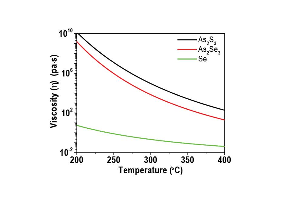
Figure 13: Temperature-dependent viscosity for various chalcogenide glasses. Typical temperature during fiber drawing for glass $\mathrm{Se,As_{2}Se_{3},As_{2}S_{3}}$ is around $220,260,300$ $\mathrm{{}^{o}C}$ with the corresponding viscosities of $10,10^{5},10^{5}$ $\mathrm{Pa\cdot s}$, respectively.

4. Diffusion term in level-set equation

To ensure numerical stability in the simulation, an artificial diffusion term proportional to a small parameter $D$ is added to level-set Eq. 5 as follows Olsson2005 ,

$$\phi_{t}+\vec{u}\cdot\vec{\nabla}\phi=D\nabla\cdot\left\{\left[1-\phi(1-\phi)\right]\nabla\phi\right\}.$$ (25)

References

- (1) J. Eggers, Rev. Mod. Phys. 69, 865 (1997).
- (2) P. de Gennes, F. Brochard-Wyart, D. Quere, Capillarity and Wetting Phenomena, Springer (2002).
- (3) A. M. Cabazat, and J. B. Fournier, Bulletin SFP, 84, 22 (1992).
- (4) J. Plateau, Acad. Sci. Bruxelles Mem. 23, 5 (1849).
- (5) L. Rayleigh, Proc. London. Math. Soc. 10, 4 (1878); L. Rayleigh, Proc. Roy. Soc. London, 29, 71 (1879); L. Rayleigh, Philos. Mag. 34, 145 (1892).
- (6) S. Tomotika. Proc. Roy. Soc. London, 150, 322 (1935).
- (7) H. A. Stone and M. P. Brenner, J. Fluid. Mech. 318, 373 (1996).
- (8) X. D. Shi, M.P. Brenner, and S. R. Nagel, Science 265, 219 (1994).
- (9) A. M. Ganan-Calvo, R. Gonzalez-Prieto, P. Riesco-Chueca, M. A. Herrada, and M. Flores-Mosquera, Nature Phys 3, 737 (2007).
- (10) M. Moseler and U. Landman, Science 289, 1165 (2000).
- (11) M. E. Toimil-Molares, A. G. Balogh, T. W. Cornelius, R. Neumann, and C. Trautmann, Appl. Phys. Lett. 85, 5337 (2004).
- (12) S. Karim, M. E. Toimil-Molares, A. G. Balogh, W. Ensinger, T. W. Cornelius, E. U. Khan, and R. Neumann, Nanotechnology 17, 5954 (2006).
- (13) J. T. Chen, M. F. Zhang, and T. P. Russell, Nano. Letter. 7, 183 (2007).
- (14) Y. Qin, S.M. Lee, A. Pan, U. Gosele, and M. Knez, Nano. Letter. 8, 114 (2008).
- (15) H. A. Stone, A.D. Stroock, and A. Ajdari, Annu. Rev. Fluid. Mech. 36, 381 (2004).
- (16) T. M. Squires and S. R. Quake, Rev. Mod. Phys. 77, 977 (2005).
- (17) R. Huang R, and Z. Suo, J. Appl. Phys. 91, 1135 (2002).
- (18) E. Cerda, K. Ravi-Chandar, and L. Mahadevan, Nature 419, 579 (2002).
- (19) E. Cerda and L. Mahadevan, Phys. Rev. Lett. 90, (2003).
- (20) A. F. Abouraddy, M. Bayindir, G. Benoit, S.D. Hart, K. Kuriki, N. Orf, O. Shapira, F. Sorin, B. Temelkuran, and Y. Fink, Nature Mater. 6, 336 (2007).
- (21) D. S. Deng, N. Orf, A. Abouraddy, A. Stolyarov, J. Joannopoulos, H. Stone, and Y. Fink, Nano. Letter. 8, 4265, (2008).
- (22) D. S. Deng, N. Orf, S. Danto, A. Abouraddy, J. Joannopoulos, and Y. Fink, Appl. Phys. Lett. 96, 23102 (2010).
- (23) S. Chandrasekhar, Hydrodynamic and Hydromagnetic Stability, Oxford University Press (1961).
- (24) J. Eggers and E. Villermaux, Rep. Prog. Phys. 71, 36601, (2008).
- (25) X. Liang, et al, manuscript in preparation.
- (26) A. D. Fitt, K. Furusawa, T. M. Monro, and C. P. Please, J. Lightwave. Technol. 19, 1924 (2001).
- (27) S. C. Xue, M. C. J. Large, G. W. Barton, R. I. Tanner, L. Poladian, and R. Lwin, J. Lightwave. Technol. 24, 853 (2006).
- (28) P. J. Roberts, F. Couny, H. Sabert, B. J. Mangan, D. P. Williams, L. Farr, M. W. Mason A. Tomlinson, T. A. Birks, J. C. Knight, and P. St. J. Russell, Opt. Express 13, 236 (2005).
- (29) I. M. Griffiths and P. D. Howell, J. Fluid Mech. 593, 181 (2007); 605, 181 (2008).
- (30) B. Temelkuran, S. D. Hart, G. Benoit, J. D. Joannopoulos, and Y. Fink, Nature 420, 650 (2002).
- (31) G. K. Batchelor, An Introduction to Fluid Dynamics, Cambridge University Press (2000).
- (32) S. D. Hart, Y. Fink, Mat. Res. Soc. Symp. Proc. 797, W.7.5.1 (2004).
- (33) S. D. Hart, Multilayer composite photonic bandgap fibers, PhD thesis, MIT (2004).
- (34) R. Scardovelli and S. Zaleski, Annu. Rev. Fluid Mech. 31, 567 (1999).
- (35) S. Osher and J. A. Sethian, J. Comput. Phys. 79, 12 (1988).
- (36) S. Osher and R. P. Fedkiw, J. Comput. Phys. 169, 463 (2001).
- (37) J. A. Sethian and P. Smereka, Annu. Rev. Fluid Mech. 35, 341 (2003).
- (38) V. F. Dobrescu and C. Radovici, Polym. Bull. 10, 134 (1983).
- (39) S. Egusa, Z.Wang, N. Chocat, Z. M. Ruff, A. M. Stolyarov, D. Shemuly, F. Sorin, P. T. Rakich, J. D. Joannopoulos and Y. Fink, Nature Mater. 9, 643 (2010).
- (40) M. F. Culpin, Proc. Phys. Soc. B70, 1069 (1957).
- (41) E. Olsson and G. A. Kreiss, J. Comput. Phys. 210, 225 (2005).
- (42) P. G. Debenedetti and F. H. Stillinger, Nature 410, 259 (2001).
- (43) A.S. Tverjanovich, Glass Phys. Chem. 29, 532 (2003).