Coexistence of single- and multi-photon processes due to longitudinal couplings between superconducting flux qubits and external fields

Abstract

In contrast to natural atoms, the potential energies for superconducting flux qubit (SFQ) circuits can be artificially controlled. When the inversion symmetry of the potential energy is broken, we find that the multi-photon processes can coexist in the multi-level SFQ circuits. Moreover, there are not only transverse but also longitudinal couplings between the external magnetic fields and the SFQs when the inversion symmetry of potential energy is broken. The longitudinal coupling would induce some new phenomena in the SFQs. Here we will show how the longitudinal coupling can result in the coexistence of multi-photon processes in a two-level system formed by a SFQ circuit. We also show that the SFQs can become transparent to the transverse coupling fields when the longitudinal coupling fields satisfy the certain conditions. We further show that the quantum Zeno effect can also be induced by the longitudinal coupling in the SFQs. Finally we clarify why the longitudinal coupling can induce coexistence and disappearance of single- and two-photon processes for a driven SFQ, which is coupled to a single-mode quantized field.

I Introduction

Superconducting quantum circuits possess discrete energy-levels and behave like natural atoms p1 ; r1 ; r2 ; r3 ; r4 ; r5 that the transitions between different energy levels can be induced by the microwave electromagnetic fields. Thus, many experiments implemented in natural atoms can also be demonstrated by using the superconducting quantum circuits, e.g., circuit quantum electrodynamics (e.g., in Refs. wallraff ; mooij1 ; review1 ), superconducting qubit dressed-states (e.g., in Refs. liudressed ; large-charge3 ; Wilson-PRB ; wallraff2009 ; greenberg ) and microwave amplification jena , state control in superconducting quantum three-level systems (e.g., in Refs. yang1 ; yang2 ; orlando2004 ; orlando2006 ; nist ; goan ; falci ; falci-1 ; ian ; Abdumalikov ), lasing without population inversion blais ; wei , cooling for the superconducting qubits (e.g., in Refs. youjqprl ; orlandon ; cooling ), and sideband excitations (e.g., in Refs. side1 ; side2 ; side3 ). In contrast to natural atoms, the potential energy of superconducting flux qubit (SFQ) circuits can be changed by adjusting externally applied magnetic fields. The tunability of potential energy makes the SFQ circuits have many features which do not exist in natural atoms.

In natural atoms, the inversion symmetry of the potential energy is given by the nature and cannot be changed artificially. Thus each eigenstate has well-defined parity, and the electric-dipole transitions induced by the electric field can only link two eigenstates which have different parities. However, the inversion symmetry of the potential energy for the SFQ circuits can be controlled by the external magnetic flux. When the inversion symmetry is adjusted to be broken, there is no well-defined parity for each eigenstate of the multi-level SFQ circuits, and the microwave-induced transitions between any two energy levels are possible, thus the multi-photon and single-photon processes can coexist for such multi-level systems. This coexistence of the multi-photon processes can be easily understood by virtue of an example using three-level SFQ circuits. That is, the transition between the ground state and the second excited state can be realized via two different pathes: (i) from the ground to the second excited state via a single-photon process; or (ii) from the ground state to the first excited state via a single-photon, and then from the first excited state to the second excited state via another single-photon process liu2005 . This means that the single- and two-photon processes can realize the same goal: the transition from the ground to the second excited state.

The coexistence liu2005 of the single- and two-photon processes in the three-level SFQ circuits with the cyclic transition, which is also called as $\Delta$-type transition in analogue to so-called $\Xi$-, $\Lambda$-, and $V$-type transitions in atomic physics or quantum optics scullybook , has been experimentally demonstrated via a delicate superconducting qubit-resonator circuit naturephysics2008 ; nano . The three-level SFQ circuits with $\Delta$-type transitions can be used to generate single photon youjqprb ; nec and cool superconducting qubits youjqprl ; orlandon . The analysis of the inversion symmetry for the potential energy of the SFQs liu2005 ; liu2006 also showed that two SFQs cannot simultaneously work at the optimal point when the frequency matching method is used to control the coupling between them. Thus either an auxiliary circuit or a coupler side1 ; plourde ; plourde-1 ; miro1 is necessary to make that both of the SFQs can be at their optimal points side1 ; liu2006 . Afterwards, several theoretical works mooij ; tsai ; miro ; franco followed proposals in Refs. side1 ; liu2006 and studied how to control the two-flux-qubit coupling using an additional nonlinear coupler, which resulted in experimental studies on controllable couplings tsaiscience and engineered selection rules for tunable couplings harrabi .

In this work, we will first show that the transverse and longitudinal couplings between the microwave fields and the SFQs can coexist. Such coexistence results from the broken inversion symmetry of tunable potential energy of the SFQ circuits. The transverse coupling between a single-mode microwave field and the SFQ, which can be reduced to the Jaynes-Cummings model in the rotating wave approximation, is well studied in the quantum optics and atomic physics scullybook . However, the model with both the transverse and longitudinal couplings is less studied. The reason is that electric-dipole induced longitudinal couplings do not exist in the natural atoms with well-defined parities. In this paper, we show some new results, which do not exist in the Jaynes-Cummings model, when both transverse and longitudinal couplings exist. Moreover, we also study the interaction between the driven SFQs and the low frequency harmonic oscillator cooling ; shnirman ; shnirman-1 when the inversion symmetry of the SFQs is broken, and further show some new phenomena due to the longitudinal coupling.

Our paper is organized as below. In Sec. II, we will briefly review the SFQ circuits. As the complementary and generalization of Ref. liu2005 , we will also clarify some points which were not studied in our earlier literatures. For instance, how to take phase transformations so that the interaction between the SFQ circuits and the external circuit can be described via the product of the loop current of the SFQ circuits and the external magnetic flux, and how the multi-photon processes can coexist in multi-level systems when the inversion symmetry is broken. In Sec. III, we will present a Hamiltonian on the transverse and longitudinal couplings between the magnetic fields and SFQs, and show how the longitudinal coupling can induce the coexistence of single- and multi-photon processes in a superconducting quantum two-level system. We will also demonstrate the longitudinal coupling induced dynamical quantum Zeno effect and the transparency of the SFQs to the transverse coupling fields. In Sec. IV, the transverse and longitudinal couplings between the driven SFQ and the low frequency harmonic oscillator (e.g., an LC circuit) is studied. We will explore the nature of the coexistence and disappearance of the single- and two-photon processes in the driven SFQs. Finally, we summarize our results in Sec. V.

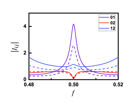
Figure 1: (Color online) Comparisons of the moduli of the $f$-dependent transition matrix elements $I_{ij}=\langle i|I|j\rangle$ with $i\neq j$ between the loop current in Eq. (3) with solid curves and those in Ref. liu2005 with dashed curves for the three lowest energy levels with $i,\,j=0,\,1,\,2$. Here, the different transition matrix elements are denoted by different colors as shown in the figure. We take $\alpha=0.8$ and $E_{\rm J}=40E_{\rm c}$ in our numerical simulations. Here, $E_{\rm c}=e^{2}/(2C_{\rm J})$.

II Theoretical model and coexistence of multi-photon processes in multi-level SFQ circuits

In this section, we first study theoretically the interaction model between the SFQ circuit with three Josephson junctions and the externally applied time-dependent magnetic flux. In the following, the abbreviation SFQ usually denotes two-level system (qubit) of the SFQ circuit if we do not specify it. As the complementary and generalization of the results in Ref. liu2005 , we will clarify some points which were not studied in the former literatures (e.g., in Refs. liu2005 ; orlando ). Then we will summarize the selection rules and discuss the coexistence of multi-photon processes in the multi-level systems.

II.1 Hamiltonian and phase transformations

Let us consider a superconducting flux qubit (SFQ) circuit, which is composed of a superconducting loop with three Josephson junctions. As in Ref. liu2005 and Ref. orlando , the two larger junctions are assumed to have equal Josephson energies $E_{\rm{J1}}=E_{\rm{J2}}=E_{\rm{J}}$ and capacitances $C_{\rm{J1}}=C_{\rm{J2}}=C_{\rm{J}}$. While for the third junction, the Josephson energy and the capacitance are assumed to be $E_{\rm J3}=\alpha E_{\rm J}$ and $C_{\rm J3}=\alpha C_{\rm J}$, with $0.5<\alpha<1$. We assume that a static magnetic flux $\Phi_{e}$ and a time-dependent magnetic flux $\Phi(t)$ are applied through the superconducting loop. In this case, the Hamiltonian can be given by

$$H=\frac{P_{p}^{2}}{2M_{p}}+\frac{P_{m}^{2}}{2M_{m}}+U(\varphi_{p},\varphi_{m})+I\Phi(t),$$ (1)

with $M_{p}=2C_{\rm J}(\Phi_{0}/2\pi)^{2}$ and $M_{m}=M_{p}(1+2\alpha)$. The potential energy $U(\varphi_{p},\varphi_{m})$ of the SFQ circuit is defined as

$$U(\varphi_{p},\varphi_{m}) = 2E_{\rm{J}}(1-\cos\varphi_{p}\cos\varphi_{m})$$ (2)

$$+ \alpha E_{\rm J}\left[1-\cos\left(2\pi f+2\varphi_{m}\right)\right],$$

with the reduced magnetic flux $f=\Phi_{e}/\Phi_{0}$ and the magnetic flux quantum $\Phi_{0}$. The third term $I\Phi(t)$ in Eq. (1) plays the similar role as the electric-dipole interactions between the nature atoms and the electric fields, and describes the interaction between the SFQ circuit and the time-dependent magnetic flux provided by the external circuit. The parameter $I$ in Eq. (1) denotes the loop current of the SFQ circuit given by liu2006

$$I=\frac{\alpha\,I_{0}}{2\alpha+1}\left[-2\sin\varphi_{m}\cos\varphi_{p}+\sin\left(2\pi f+2\varphi_{m}\right)\right],$$ (3)

when the time-dependent magnetic flux $\Phi(t)=0$, here $I_{0}=2\pi E_{\rm J}/\Phi_{0}$. We note that Eq. (3) is different from those in the former literatures (e.g., in Refs. liu2005 ; youjq ). This difference results from different phase transformations

$$\phi_{p} = \frac{1}{2}(\phi_{1}+\phi_{2}),$$ (4)

$$\phi_{m} = \frac{1}{2}(\phi_{2}-\phi_{1})+\frac{2\pi\alpha}{(1+2\alpha)}\frac{\Phi(t)}{\Phi_{0}},$$ (5)

with the superconducting phase differences $\phi_{1}$ and $\phi_{2}$ of the two identical Josephson junctions. We also use the phase constraint condition for superconducting phase differences $\phi_{i}$ (with $i=1,\,2,\,3$) of the three Josephson junctions as

$$-\phi_{1}+\phi_{2}+\phi_{3}+\frac{2\pi\Phi_{e}}{\Phi_{0}}+\frac{2\pi\Phi(t)}{\Phi_{0}}=0,$$ (6)

when Eqs. (2) and (3) are derived.

In the former literatures (e.g., in Refs. liu2005 ; youjq ), the second term in Eq. (5) for the phase transformations has been neglected. Our derivation here and the former derivation in the literatures liu2005 ; youjq can give the same type of the interaction Hamiltonian between the time-dependent magnetic flux and the superconducting flux qubit circuit, but there is a significant difference. In the derivation of Refs. liu2005 ; youjq , $I$ in Eq. (1) is the supercurrent passing through one of the three Josephson junctions. But for our derivation here, $I$ in Eq. (1) is the loop current of the SFQ circuit. Thus two derivations result in different coupling strengths between the SFQ circuit and the external magnetic flux. We think that the phase transformations in Eqs. (4) and (5) are more appropriate than those used in the former literatures (e.g., in Refs. liu2005 ; youjq ) when the time-dependent magnetic flux is considered. Because in this transformation, the interaction between the SFQ circuit and the external circuit can be expressed as the product liu2006 of the loop current $I$ of the SFQ circuit and the external magnetic flux $\Phi(t)$ provided by the external circuit. This is in accordance with the interaction energy between the circulating current in a metal loop and the external magnetic flux.

We know that the loop current of the SFQ circuit equals to the summation of the supercurrent and the displacement current through one of the three Josephson junctions. The phase transformations in the former literatures liu2005 ; youjq result in an approximated current-flux interaction Hamiltonian between the SFQ circuit and the external magnetic flux $\Phi(t)$, because the displacement currents in the three Josephson junctions are simply neglected. However, the phase transformations, used in Eqs. (4) and (5), result in that $I$ in Eq. (1) is just the loop current given in Eq. (3), which is calculated by including both the supercurrent and the displacement current for each junction. Thus the phase transformations, used in Eqs. (4) and (5), overcome the drawback of former derivations liu2005 ; youjq and are more reasonable.

We should also note that the transformations applied in Eqs. (4) and (5) do not change the basic results on the selection rules and the adiabatic control of the quantum states that were studied in Ref. liu2005 in which the displacement currents are neglected. This can be very easily verified by using Eq. (2) and Eq. (3), that is: (i) when $f=0.5$ which is called as an optimal point, the potential energy in Eq. (2) is an even function of the variables $\phi_{p}$ and $\phi_{m}$, and the loop current in Eq. (3) is an odd function of the variables $\phi_{m}$ and $\phi_{p}$. Therefore the potential energy and the loop current have the well-defined symmetry. (ii) When $f\neq 0.5$, the inversion symmetries for both the potential energy in Eq. (2) and the loop current in Eq. (3) do not exist. Therefore, the conclusions in both (i) and (ii) are the same as those in Refs. liu2005 ; youjq . However due to the different expressions of the loop currents in Eq. (3) and in Refs. liu2005 ; youjq , the transition matrix elements will be re-normalized. Below we will further clarify this conclusion via the discussions on the selection rules and numerical calculations for the transition matrix elements.

Table 1: Comparison between SFQ circuits and natural atoms for dipole moments, parities, symmetry, and selection rules.

Atoms	Dipole moments	Parities	Symmetry	Selection rules
Natural atoms	$\propto e\overrightarrow{r}$	Odd	Well-defined	Have
SQC ($f=0.5$)	$\begin{array}[]{c}\propto-\sin(2\varphi_{m})\\ -2\sin\varphi_{m}\cos\varphi_{p}\end{array}$	Odd	Well-defined	Have
SQC ($f\neq 0.5$)	$\begin{array}[]{c}\propto\sin(2\varphi_{m}+2\pi f)\\ -2\sin\varphi_{m}\cos\varphi_{p}\end{array}$	No parity	Broken	Not have

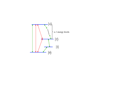
Figure 2: (Color online) Schematic diagram for the coexistence of different photon transition processes when the inversion symmetry of the potential energy is broken, i.e., $f\neq 0.5$. In this case, all of the transitions between any two energy levels are possible, i.e., there is no forbidden transition. For example, the loop formed by three red arrow lines (which link to ground state, the second excited state, and the $n$th excited state) denotes a coexistence of single- and two-photon processes for the $(n+1)$-level system. The coexistence of single- and two-photon processes can also be formed by the ground, first excited, and second excited states. However, the loop formed by the green arrow lines (which link the ground, second, third, until $n$th excited states) denotes a coexistence of single- and $n$-photon processes for the $(n+1)$-level system. This schematic diagram also shows that many different photon processes can coexist in the SFQ circuit with the broken inversion symmetry.

II.2 Selection rules and coexistence of multi-photon processes in $n$-level systems

As a necessary supplementary and generalization of the results in Ref. liu2005 for the microwave-induced transitions between two different energy levels, we now rewrite the Hamiltonian in Eq. (1) using eigenstates $\{|i\rangle,\,i=0,\,\cdots n\}$ of the SFQ circuits as the basis

$$H=\sum_{i}\hbar\omega_{ii}|i\rangle\langle i|+\sum_{i,j=0}^{n}I_{ij}|i\rangle\langle j|\Phi(t)\;,$$ (7)

with “dipole” matrix elements $I_{ij}=\langle i|I|j\rangle$ and the eigenvalue $\hbar\omega_{ii}$ of the eigenstate $|i\rangle$.

As discussed above for $f=0.5$, the potential energy in Eq. (2) and the loop current in Eq. (3) have inversion symmetries, and also all eigenstates of the SFQ circuit have well-defined parities. The loop current $I$ in Eq. (3) is an odd function of the variables $\phi_{p}$ and $\phi_{m}$. Therefore, at the point $f=0.5$, the SFQ circuit has the same selection rules as the natural atoms, and the microwave-induced transition can only link two states which have different parities. However, the symmetry is broken when $f\neq 0.5$. Thus the selection rules of the SFQ circuits do not exist, and the microwave-induced transitions between any two energy levels are possible. The comparison of the selection rules between the SFQ circuits and natural atoms is summarized in Table 1.

To compare the $f$-dependent transition matrix elements using the loop current in Eq. (3) with those in, e.g., Ref. liu2005 , the moduli of the transition matrix elements $I_{ij}=\langle i|I|j\rangle$ versus the reduced magnetic flux $f$ is plotted in Fig. 1 for the three lowest energy levels with $i,\,j=0,\,1,\,2$ and $i\neq j$. Numerical results in Fig. 1 clearly show that there is the same transition rule for the current operator used in Eq. (3) and in Ref. liu2005 . However, as shown in Fig. 1, the amplitudes of the transition matrix elements are different for the two different current expressions in Eq. (3) and in Ref. liu2005 . It is obvious that the coupling strength given by our theoretical derivation here is bigger than that given in Ref. liu2005 near the optimal point.

As shown in Table 1 and Fig. 1, when the inversion symmetry of the potential energy is broken (i.e., $f\neq 0.5$), all transition matrix elements are nonzero, thus the transitions between any two levels are allowed. In this case, the single- and $n$-photon processes can coexist for the $(n+1)$-level SFQ circuit. That is, for an $(n+1)$-level system, the transition from the ground state $|0\rangle$ to the $n$th excited state $|n\rangle$ can be realized by either the single-photon process ($|0\rangle\rightarrow|n\rangle$) or the $n$-photon processes ($|0\rangle\rightarrow|1\rangle\rightarrow\cdots|n-1\rangle\rightarrow|n\rangle$). Similarly, many different photon processes can also coexist in the case with the broken inversion symmetry. The coexistence of single- and $n$-photon processes has been schematically shown in Fig. 2. When $n=2$, we have the three-level SFQ circuit as discussed in Ref. liu2005 , then the single- and two-photon processes can coexist. It should be noted that the transitions between two energy levels should obey the selection rules at the optimal point $f=0.5$. The photon transition processes for the $(n+1)$-level SFQ circuit have been schematically shown in Fig. 3 for the case $f=0.5$.

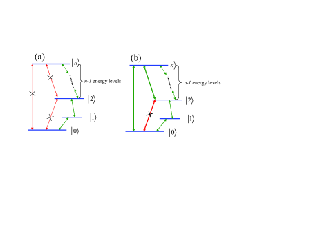
Figure 3: (Color online) The Schematic diagram for the photon transition processes when the inversion symmetry of the potential energy is well-defined, i.e., $f=0.5$. For convenience, let us assume that the microwave-induced transition between the state $|n\rangle$ and the state $|n+1\rangle$ is possible for the $(n+1)$-level system. Therefore, it is clear that the transition between the state $|0\rangle$ and the state $|2\rangle$ is prohibited. In (a), if the transition between the state $|2\rangle$ and the state $|n\rangle$ is prohibited, then the transition between the state $|n\rangle$ and the state $|0\rangle$ is also prohibited; In (b), if the transition between the state $|2\rangle$ and the state $|n\rangle$ is allowed, then the transition between the state $|n\rangle$ and the state $|0\rangle$ is also allowed, however the transition between the state $|0\rangle$ and the state $|2\rangle$ is forbidden. In both figures, the sign “$\times$” denotes that the electric-dipole-like microwave-induced transition is prohibited. Because the parities for those states are the same.

In above, we mainly analyze the basic properties of the multi-level SFQ circuits. Below we will focus on new features of the SFQ (or quantum two-level system formed by the superconducting flux qubit circuit) when the inversion symmetry of the potential energy is broken.

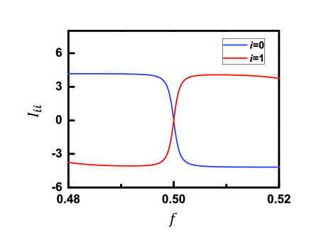
Figure 4: (Color online) The $f$-dependent loop current $I_{ii}=\langle i|I|i\rangle$ for the two lowest energy levels $|0\rangle$ and $|1\rangle$. Here, we take the typical numbers $\alpha=0.8$ and $E_{\rm J}=40E_{\rm c}$ in our numerical simulations.

III New phenomena induced by longitudinal couplings between SFQs and external magnetic fluxes

III.1 Theoretical model on the couplings between SFQs and external magnetic fluxes

Let us consider the case of the two lowest energy levels for the SFQ circuits, i.e., $n=1$. In this case, the Hamiltonian in Eq. (7) is reduced to that of the superconducting flux qubits (SFQs), driven by the time-dependent external magnetic flux. In Fig. 4, the matrix elements of the loop current $I$ of the SFQs for the two lowest energy levels $|0\rangle$ and $|1\rangle$ are plotted versus the reduced magnetic flux $f$. Fig. 4 shows a well-known result that the loop current $I$ in the ground $|0\rangle$ and the first excited $|1\rangle$ states are zero at the optimal point $f=0.5$. However, once the symmetry is broken, the loop current for both states are nonzero. We note that the loop current $I_{ii}$ also depends on the ratios $\alpha=E_{\rm J3}/E_{\rm J1}$ and $E_{\rm J}/E_{\rm c}$. As shown in Fig. 4, the loop current $I_{ii}$ is almost a constant for $\alpha=0.8$ and $E_{\rm J}/E_{\rm c}=40$ when $f$ deviates from $0.5$, however it is not always the case for other parameter ratios.

Based on the above discussions, for a SFQ interacting with the time-dependent magnetic flux, we have the following general Hamiltonian

$$H = \sum_{i=0}^{1}\hbar\omega_{ii}(f)|i\rangle\langle i|+\left[I_{01}(f)|0\rangle\langle 1|+I_{10}(f)|1\rangle\langle 0|\right]\Phi(t)$$ (8)

$$+ \left[I_{00}(f)|0\rangle\langle 0|+I_{11}(f)|1\rangle\langle 1|\right]\Phi(t).$$

Here, we write $\omega_{ii}(f)$ and $I_{ij}(f)$ (with $i,\,j=0,\,1$) to emphasize the $f$-dependent parameters.

Let us now first discuss the interaction between the SFQ and the classical magnetic flux $\Phi(t)$ using the Hamiltonian in Eq. (8) when $f=0.5$. The above analytical analysis together with Fig. 1 and Fig. 4 show

$$I_{00}(f=0.5)=I_{11}(f=0.5)=0,$$ (9)

and

$$I_{10}(f=0.5)=I_{01}(f=0.5)\neq 0.$$ (10)

Therefore, in Eq. (8), the two coupling terms become

$$I_{ii}(f=0.5)|i\rangle\langle i|\Phi(t)=0,$$ (11)

with $i=0,\,1$, which means that there is no longitudinal coupling between the time-dependent magnetic flux and the SFQ at the optimal point. There are only coupling terms $I_{01}(f=0.5)(|0\rangle\langle 1|+|1\rangle\langle 0|)\Phi(t)$ in Eq. (8), called as the transverse coupling between the time-dependent magnetic flux and the SFQ. Therefore, under the rotating wave approximation, the Hamiltonian in Eq. (8) at the optimal point can further be reduced to the Jaynes-Cumming model, which has been extensively explored in the quantum optics and the circuit QED system.

When $f\neq 0.5$, all elements $I_{ij}(f)$ with $i=0,\,1$ are nonzero. In this case, the interaction Hamiltonian between the time-dependent magnetic flux and the SFQs includes both the transverse and longitudinal couplings, which are less studied. This longitudinal coupling can induce some unusual phenomena which will be explored below. For convenience, our studies below just consider the case of the longitudinal and transverse couplings between a driving classical field and a SFQ, however all of the discussions in the subsections III.2, III.3, and III.4 can be applied to the case with many driving fields.

III.2 Longitudinal coupling induced coexistence of single- and multi-photon processes in SFQs

For convenience, using the relations in Eqs. (9) and (10), the Hamiltonian in Eq. (8) can be rewritten as

$$H=\hbar\frac{\omega_{q}}{2}\sigma_{z}+\hbar(\lambda_{x}\sigma_{x}+\lambda_{z}\sigma_{z})\cos(\omega_{0}t),$$ (12)

with $\sigma_{z}=|1\rangle\langle 1|-|0\rangle\langle 0|$ and $\sigma_{x}=|0\rangle\langle 1|+|1\rangle\langle 0|$. Here, we assume the magnetic flux $\Phi(t)$ in Eq. (8) to be $\Phi(t)=\Phi\cos(\omega_{0}t)$, and then $\lambda_{x}=\Phi I_{01}/\hbar$ and $\lambda_{z}=\Phi(I_{11}-I_{00})/(2\hbar)$.

If the SFQ works at the optimal point (i.e., $f=0.5$), then $I_{11}(f=0.5)=0$ which implies the longitudinal coupling constant $\lambda_{z}=0$. In this case, Eq. (12) becomes a standard Hamiltonian of a driven SFQ, and there is only single-photon resonant transition in the SFQ induced by the external magnetic flux with the condition $\omega_{q}=\omega_{0}$.

When the reduced magnetic flux deviates from the optimal point, i.e., $f\neq 0.5$, there are both the transverse and longitudinal couplings between the SFQ and the external magnetic flux. In contrast to the case of only the single-photon process for the transverse coupling between the SFQ and the external magnetic flux, the longitudinal coupling can result in the coexistence of the single- and multi-photon processes in the SFQs. To demonstrate this, we now apply a unitary transformation

$$U(t)=\exp\left[-\frac{i}{2}\left(\omega_{0}t+2\frac{\lambda_{z}}{\omega_{0}}\sin\omega_{0}t\right)\sigma_{z}\right]$$ (13)

to Eq. (12), and thus the Hamiltonian in Eq. (12) becomes

$$H = \hbar\frac{\omega_{q}-\omega_{0}}{2}\sigma_{z}+\hbar\sum_{n}\left[\lambda_{n}e^{-in\omega_{0}t}\sigma_{+}+{\rm h.c.}\right],$$ (14)

under the rotating wave approximation. The effective Rabi frequency in Eq. (14) is given by

$$\lambda_{n}=\lambda_{x}J_{n}\left[\frac{2\lambda_{z}}{\omega_{0}}\right],$$ (15)

which depends on both $\lambda_{z}$ and $\omega_{0}$ with the Bessel functions $J_{n}(2\lambda_{z}/\omega_{0})$ of the first kind. When deriving Eq. (14), we use the relation

$$\exp\left[i\frac{2\lambda_{z}}{\omega_{0}}\sin(\omega_{0}t)\right]=\sum_{n=-\infty}^{n=\infty}J_{n}\left[\frac{2\lambda_{z}}{\omega_{0}}\right]\exp\left[in\omega_{0}t\right].$$ (16)

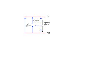
Figure 5: (Color online) Schematic diagram for the longitudinal coupling induced coexistence of multi-photon processes in the SFQs

We note if the SFQ works at the optimal point, then $\lambda_{z}=0$ and the Bessel functions

$$J_{n\neq 0}\left(\frac{2\lambda_{z}}{\omega_{0}}=0\right) = 0,$$ (17)

$$J_{n=0}\left(\frac{2\lambda_{z}}{\omega_{0}}=0\right) = 1.$$ (18)

In this case, Eq. (14) is reduced to the usual Jaynes-Cumming model for the externally driven two-level system, and only describes the single-photon resonant transition with the condition $\omega_{q}=\omega_{0}$. The single-photon process is characterized by the term for $n=0$ in Eq. (14) with the amplitude

$$\lambda_{0}=\lambda_{x}J_{0}\left(\frac{2\lambda_{z}}{\omega_{0}}=0\right)=\lambda_{x}.$$ (19)

This is also an obvious result of Eq. (12) for $\lambda_{z}=0$ and with the rotating wave approximation as described above.

However, for the case $\lambda_{z}\neq 0$, all of the Bessel functions $J_{n}(2\lambda_{z}/\omega_{0})$ and then $\lambda_{n}$ are nonzero except some special ratios $2\lambda_{z}/\omega_{0}$, which are roots of the Bessel functions. For nonzero $\lambda_{n}$, Eq.  (14) shows an obvious resonant condition

$$\omega_{q}=(n+1)\omega_{0}.$$ (20)

Therefore when the inversion symmetry is broken, the longitudinal coupling can induce the coexistence of single- and multi-photon processes in the SFQ. The coexistence of single- and multi-photon processes in the SFQs is schematically shown in Fig. 5.

In summary, the conditions for the coexistence of single- and multi-photon processes in the SFQs are: (a) the SFQs do not work at the optimal point, and thus there are both the longitudinal and transverse couplings between the SFQs and the external magnetic fluxes; (b) the ratios $2\lambda_{z}/\omega_{0}$ are not roots of the function $J_{n}(2\lambda_{z}/\omega_{0})$. The multi-photon processes in the SFQs with the driving fields large2 have been experimentally observed (e.g., in Refs. multi1 ; multi2 ; large1 ; berns ; large3 ). Thus the above two conditions and our studies here should be necessarily theoretical complementary to these experimental studies (e.g., in Refs. multi1 ; multi2 ; large1 ; berns ; large3 ).

We notice that the Hamiltonian used in Eq. (12) is equivalent to one, commonly used in the literatures (e.g., Refs. multi1 ; multi2 ) for SFQs, described by

$$H^{\prime}=\varepsilon\sigma_{z}+\Delta\sigma_{x}+\lambda\sigma_{z}\cos(\omega_{0}t),$$ (21)

in the loop current basis. Because Eq. (21) can be easily transformed to Eq. (12) in the qubit basis by diagonalizing the first two terms of Eq. (21). We also note that the longitudinal coupling induced coexistence of multi-photon processes in SFQs actually bears similarity to the phenomenon of coherent destruction of tunneling CDT1 ; CDT2 .

III.3 Longitudinal coupling induced transparency of the SFQs to the transverse coupling fields

We now show how the longitudinal coupling field can result in the transparency of the SFQ to the transverse coupling fields. Let us first give the solutions of the Hamiltonian in Eq. (14). We assume that the solutions $|\Psi\rangle$ of Eq. (14) have the following form

$$|\Psi\rangle=A(t)|0\rangle+B(t)|1\rangle.$$ (22)

According to the expansion of the Hamiltonian in Eq. (14), there are many resonant peaks under the frequency matching condition $\omega_{q}=(n+1)\omega_{0}$. If we assume that the frequency of the driving field satisfies the condition $\omega_{0}=\omega_{q}/(n+1)$, then the time-dependent parameters $A(t)$ and $B(t)$ can be given by

$$A(t) = \left\{A(0)\left[\cos\left(\frac{\Omega_{n}t}{2}\right)-i\frac{\Delta_{n}}{\Omega_{n}}\sin\left(\frac{\Omega_{n}t}{2}\right)\right]\right.$$ (23)

$$- \left.iB(0)\frac{2\lambda_{n}}{\Omega_{n}}\sin\left(\frac{\Omega_{n}t}{2}\right)\right\}\exp\left[i\frac{n\omega_{0}t}{2}\right],$$

$$B(t) = \left\{B(0)\left[\cos\left(\frac{\Omega_{n}t}{2}\right)+i\frac{\Delta_{n}}{\Omega_{n}}\sin\left(\frac{\Omega_{n}t}{2}\right)\right]\right.$$ (24)

$$- \left.iA(0)\frac{2\lambda_{n}}{\Omega_{n}}\sin\left(\frac{\Omega_{n}t}{2}\right)\right\}\exp\left[-i\frac{n\omega_{0}t}{2}\right].$$

Here, $A(0)$ and $B(0)$ are given by the initial conditions of Eq. (22). The Rabi frequency $\Omega_{n}$ and the parameter $\Delta_{n}$ are given by

$$\Omega_{n} = \sqrt{\Delta_{n}^{2}+4|\lambda_{n}|^{2}},$$ (25)

$$\Delta_{n} = \omega_{q}-(n+1)\omega_{0}.$$ (26)

If the SFQ is initially prepared to the ground state, i.e., $A(0)=1$, and also the coupling constant $\lambda_{n}$ satisfies the condition $\lambda_{n}=0$, then from Eqs. (23) and (24), we can obtain $|B(t)|\equiv 0$ and $|A(t)|\equiv 1$. In this case, the SFQ is always in its ground state and the population in the excited state is always zero even that the resonant condition $\omega_{q}=(n+1)\omega_{0}$ is satisfied. This means that the SFQ is transparent to the transverse field due to the longitudinal coupling. However, when the longitudinal coupling is zero, once the resonant condition is satisfied, the transverse field can be absorbed by the SFQ.

III.4 Longitudinal coupling induced dynamical quantum Zeno effect

We now study another interesting phenomenon, that is, the environmental effect of the flux qubit can be switched off by virtue of the longitudinal coupling field when the inversion symmetry of the SFQ potential energy is broken. The Hamiltonian of the driven SFQ interacting with the environment can be written as

$$H_{\rm en} = \hbar\frac{\omega_{q}}{2}\sigma_{z}+\hbar(\lambda_{x}\sigma_{x}+\lambda_{z}\sigma_{z})\cos(\omega_{0}t)$$ (27)

$$+ \sum_{i}\hbar\omega_{i}b^{\dagger}_{i}b_{i}+\hbar\sum_{i}(g_{i}\sigma_{+}b_{i}+g^{*}_{i}\sigma_{-}b^{\dagger}_{i}),$$

with the definition $\sigma_{x}=\sigma_{+}+\sigma_{-}$ for the ladder operators $\sigma_{\pm}$. Here, as in Eq. (12), the longitudinal and transverse couplings between the SFQ and the classical fields are characterized by the parameters $\lambda_{z}$ and $\lambda_{x}$. The environment is presented as a set of harmonic oscillators, each with the frequency $\omega_{i}$ and the creation (annihilation) operator $b_{i}^{\dagger}$ ($b_{i}$). The coupling constant between the SFQ and the $i$th bosonic mode is denoted by $g_{i}$. If a unitary transformation as in Eq. (13) is applied to the Hamiltonian in Eq. (27), then we have an effective Hamiltonian

$$H_{\rm en}^{\rm eff} = \hbar\frac{\omega_{q}-\omega_{0}}{2}\sigma_{z}+\hbar\sum_{n}\left[\lambda_{n}e^{-in\omega_{0}t}\sigma_{+}+{\rm h.c.}\right]$$

$$+ \sum_{i}\hbar\omega_{i}b^{\dagger}_{i}b_{i}+\hbar\sum_{n}\sum_{i}(g_{i}^{(n)}\sigma_{+}b+g^{(n)*}_{i}\sigma_{-}b^{\dagger}),$$

with

$$g_{i}^{(n)}=g_{i}\,J_{n}\left(\frac{2\lambda_{z}}{\omega_{0}}\right)\exp\left[i(n+1)\omega_{0}t\right].$$ (29)

Here, $J_{n}(2\lambda_{z}/{\omega_{0}})$ and $\lambda_{n}$ are given in Eq. (15).

For a modulation of frequency $\omega_{0}$ with the resonant $\omega_{q}=(n+1)\omega_{0}$ or near resonant condition $\omega_{q}\approx(n+1)\omega_{0}$, here $n=[\omega_{q}/\omega_{0}]-1$ denotes the integer nearest to $(\omega_{q}/\omega_{0})-1$. Then under the rotating wave approximation with neglecting fast oscillating terms rotating , we only take the term with the integer number $n=[\omega_{q}/\omega_{0}]-1$, and then the Hamiltonian in Eq. (III.4) becomes

$$H_{\rm en}^{\rm eff} = \hbar\frac{\omega_{q}-\omega_{0}}{2}\sigma_{z}+\sum_{i}\hbar\omega_{i}b^{\dagger}_{i}b_{i}$$

$$+ \hbar\left[\lambda_{[\frac{\omega_{q}}{\omega_{0}}]-1}\exp\left\{-i\left(\left[\frac{\omega_{q}}{\omega_{0}}\right]-1\right)\omega_{0}t\right\}\sigma_{+}+{\rm h.c.}\right]$$

$$+ \hbar\sum_{i}(g_{i}^{\left([\frac{\omega_{q}}{\omega_{0}}]-1\right)}\sigma_{+}b+{\rm h.c.}).$$

Equation (III.4) clearly shows that the SFQ is decoupled from its environment when the ratio $2\lambda_{z}/\omega_{0}$ is one of the zeros of the Bessel function $J_{[\omega_{q}/\omega_{0}]-1}\left(2\lambda_{z}/\omega_{0}\right)$, because the coupling constants $\lambda_{[\omega_{q}/\omega_{0}]-1}=0$ and $g_{i}^{\left([\omega_{q}/\omega_{0}]-1\right)}=0$ at the zeros of the Bessel functions. Therefore, in contrast to the longitudinal coupling induced transparency, if the SFQ is initially prepared to the excited state, i.e., $B(0)=1$, then $|B(t)|\equiv 1$ and $|A(t)|\equiv 0$. In this case, the SFQ evolves freely and is always in its excited state, which is equivalent to a dynamical quantum Zeno effect peres ; lanzhou .

IV Coupling between a driven SFQ and an LC circuit with low frequency

IV.1 Theoretical model

As shown in the red dashed box of Fig. 6, we first consider the interaction between a SFQ and a quantized low frequency LC circuit (e.g., Refs. naturephysics2008 ; shnirman ) with the frequency $\omega$. The Hamiltonian can be given by

$$H_{q}=\sum_{i=0}^{1}\hbar\omega_{ii}|i\rangle\langle i|+\hbar\omega a^{\dagger}a+M\sqrt{\frac{\hbar\omega}{2L}}\sum_{i,j=0}^{1}I_{ij}|j\rangle\langle i|(a+a^{\dagger}),$$ (31)

which can be further written as

$$H_{q}=\hbar\frac{\omega_{q}}{2}\sigma_{z}+\hbar\omega a^{\dagger}a+\hbar\left(g_{1}\sigma_{x}+g_{2}\sigma_{z}\right)(a+a^{\dagger}),$$ (32)

with the coefficients

$$g_{1} = \frac{M}{\hbar}\sqrt{\frac{\hbar\omega}{2L}}I_{01},$$ (33)

$$g_{2} = \frac{M}{2\hbar}\sqrt{\frac{\hbar\omega}{2L}}(I_{11}-I_{00}).$$ (34)

Here, $M$ is the mutual inductance between the LC circuit and the SFQ. $L$ is the self-inductance of the LC circuit. $a$ ($a^{\dagger}$) is the annihilation (creation) operator of the quantized LC circuit. And the condition $I_{01}=I_{10}$ is used. The transverse and longitudinal couplings of the SFQ to the LC circuit are realized via the coupling constants $g_{1}$ and $g_{2}$. The analysis of the inversion symmetry of the SFQ potential energy tells us that the longitudinal coupling vanishes (i.e., $g_{2}=0$) only at the optimal point $f=0.5$, however the transverse coupling is always nonzero. Below, we will study the case that both transverse and longitudinal coupling terms are nonzero for the reduced magnetic flux $f\neq 0.5$.

As in experiments naturephysics2008 ; cooling and also theoretical studies in Ref. shnirman , we now consider that the LC circuit and the SFQ are in the regime of the very large detuning, i.e., the dispersive regime

$$\Delta=\omega_{q}-\omega\gg|g_{1}|.$$ (35)

In this condition, for the simplicity of the discussions, we take an approximation

$$\omega_{q}-\omega\approx\omega_{q}+\omega,$$ (36)

and apply a unitary transformation $U=\exp(-iS)$ to Eq. (32) with

$$S=\frac{g_{1}}{\omega_{q}}(a^{\dagger}+a)\sigma_{y},$$ (37)

then we have an effective Hamiltonian

$$H_{q}^{\rm eff} = U^{\dagger}H_{q}U\approx\hbar\frac{\omega_{q}}{2}\sigma_{z}+\hbar\omega a^{\dagger}a$$ (38)

$$+ \hbar\sigma_{z}\left[g_{2}-\frac{g^{2}_{1}}{\omega_{q}}(a^{\dagger}+a)\right](a^{\dagger}+a),$$

which has been obtained in Ref. shnirman . Here, we only keep to the first order of $g_{1}/\Delta$. As discussed in Ref. shnirman , this transform considers that the transverse coupling affects the SFQ via a second-order longitudinal coupling.

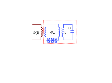
Figure 6: (Color online) Schematic diagram for the coupling between an LC circuit and an SFQ (indicated by the red dashed box), which is driven by the external magnetic flux $\Phi(t)$ (left part of the figure with the dark red color).

IV.2 Single- and two-photon coupling between the low frequency oscillator and the driven SFQ

Let us now discuss the coexistence and disappearance of single- and two-photon processes in the driven SFQs when the longitudinal coupling appears. As shown in Fig. 6, we assume that a classical magnetic flux $\Phi(t)$ with the frequency $\omega_{0}$ is applied to the SFQ, which is coupled to an LC circuit. We consider a general case for the reduced magnetic flux $f\neq 0.5$. In this case, the classical field has both the transverse and longitudinal couplings to the SFQ via the operators $\sigma_{x}$ and $\sigma_{z}$. The total Hamiltonian can be given by

$$H_{T}=H_{q}+\hbar(\lambda_{x}\,\sigma_{x}+\lambda_{z}\sigma_{z})\cos(\omega_{0}t).$$ (39)

As for obtaining Eq. (38), we first apply the unitary transformation $U=\exp(-iS)$ to Eq. (39), then we obtain an effective Hamiltonian

$$H^{\rm eff}_{T}=H^{\rm eff}_{q}+\hbar(\lambda_{x}\,\sigma_{x}+\lambda_{z}\sigma_{z})\cos(\omega_{0}t).$$ (40)

Here, we have neglected the three-body coupling terms between the LC circuit, the SFQ, and the classical magnetic flux by taking an approximation similar to that in Ref. shnirman . When Eq. (40) is derived, all of the nonresonant conditions have to be satisfied. However, in contrast to the Ref. shnirman where only the transverse coupling term is kept, here we keep both the longitudinal and transverse couplings between the classical field and the SFQ. Let us now further apply another unitary transformation

$$U(t)=\exp\left[\frac{i}{2}\left(\omega_{0}t+2\frac{\lambda_{z}}{\omega_{0}}\sin\omega_{0}t\right)\sigma_{z}\right]$$ (41)

to Eq. (40), then we have

$$H^{\rm eff}_{T} = \hbar\frac{\omega_{q}-\omega_{0}}{2}\sigma_{z}+\hbar\sigma_{z}\left[g_{2}+\frac{g^{2}_{1}}{\Delta}(a^{\dagger}+a)\right](a^{\dagger}+a)$$ (42)

$$+ \hbar\omega a^{\dagger}a+\hbar\sum_{n}\left[\lambda_{n}e^{-in\omega_{0}t}\sigma_{+}+{\rm h.c.}\right],$$

with the effective Rabi frequency $\lambda_{n}=\lambda_{x}J_{n}(2\lambda_{z}/\omega_{0})$. For the last term in the righthand side of Eq. (42), only the term for $n=0$ with the Rabi frequency $\lambda_{0}=\lambda_{x}J_{0}(2\lambda_{z}/\omega_{0})$ is time independent.

We assume that $\omega_{q}\approx(n+1)\omega_{0}$. In the rotating reference frame $V(t)=\exp(-in\omega_{0}\sigma_{z}t/2)$ and using the dressed SFQ basis, Eq. (42) becomes

$$H_{\rm T,R}^{\rm eff}=\hbar\frac{\Omega_{\rm R}}{2}\sigma_{z}+\hbar\omega a^{\dagger}a+\hbar(\beta_{1}\sigma_{+}a+\beta_{2}\sigma_{+}a^{2}+{\rm h.c.}),$$ (43)

with the dressed qubit frequency

$$\Omega_{\rm R}=\sqrt{[\omega_{q}-(n+1)\omega_{0}]^{2}+(2\lambda_{n})^{2}}.$$ (44)

Here, the fast oscillating terms in Eq. (42) and the anti-rotating terms in the dressed SFQ basis have been neglected. The subscript “R” indicates the rotating reference frame. The coupling constants $\beta_{1}$ and $\beta_{2}$ are

$$\beta_{1} = 2\frac{\lambda_{n}}{\Omega_{\rm R}}g_{2},$$ (45)

$$\beta_{2} = 2\frac{\lambda_{n}g^{2}_{1}}{\Omega_{\rm R}\Delta}.$$ (46)

Equation (43) shows that the single-photon process survives when $\Omega_{\rm R}=\omega$, however two-photon process appears when $\Omega_{\rm R}=2\omega$.

For the single- and two-photon processes in the driven SFQ shown above, we should notice: (i) if the driven SFQ works at the optimal point $f=0.5$, then $g_{2}=0$ and the Hamiltonian in Eq. (32) is reduced to that of the Jaynes-Cumming model. In this case, $\beta_{1}=0$ in Eq. (43) and only the two-photon process exists. However, if $f\neq 0.5$, which corresponds to the broken inversion symmetry of the SFQ potential energy, then both $g_{1}$ and $g_{2}$ are nonzero. In this case, $\beta_{1}$ and $\beta_{2}$ in Eq. (43) take nonzero values, thus single- and two-photon processes can coexist. (ii) Eq. (43) also shows that both $\beta_{1}$ and $\beta_{2}$ are proportional to the $n$th Bessel functions $J_{n}(2\lambda_{z}/\omega_{0})$. In the case of zeros of the $n$th Bessel functions, the transverse coupling via $\sigma_{x}$ between the driven SFQ and the LC circuit is switched off, neither single-photon process nor two-photon process can be observed in the driven SFQ. This is an additional condition to obtain the coexistence of single- and two-photon processes in the driven SFQ naturephysics2008 . Therefore, the ratio between the longitudinal coupling constant $\lambda_{z}$ and the frequency $\omega_{0}$ of the driving field determines the coexistence and disappearance of single- and two-photon processes. (iii) Due to the coexistence of single- and two-photon processes when the inversion symmetry of the SFQ potential energy is broken, the preparation and engineering of quantum states of the harmonic oscillator can be more efficient yjzhao . (iv) As the closing remark of this section, we also note that the dynamics of the SFQ and the LC oscillator in the dispersive regime beyond the rotating-wave approximation has been studied in Ref. zueco . This method can also be applied to the derivation in Eq. (38) when the rotating wave approximation cannot be made.

V Conclusions and Discussions

In summary, as the necessary complementary and generalization of our earlier studies liu2005 , we first give phase transformations when the time-dependent microwave is applied, and then study the microwave-induced transitions between different energy levels in the multi-level systems formed by the SFQ circuits. We have compared the selection rules between these superconducting artificial “atoms” and the natural atoms. It is found that the selection rules for such multi-level systems are the same as those of the multi-level natural atoms when the reduced bias magnetic flux $f$, applied to the superconducting loop of the SFQ circuits, is at the optimal point $f=0.5$. This is because the inversion symmetry of the potential energy is well defined in this case. However, when the reduced bias magnetic flux is not at the optimal point, i.e., $f\neq 0.5$, the superconducting “atoms” have no selection rules, in this case, the microwave-induced transitions between any two energy levels are possible.

The inversion symmetry of the potential energy for the SFQ circuits is not only important to the multi-level systems, but also important to the two-level systems (qubits). With the broken inversion symmetry, there are both the transverse and longitudinal couplings between the SFQs and the external magnetic fluxes. Compared with the two-level natural atoms that only have the transverse coupling, the SFQs have several new phenomena due to the existence of additional longitudinal couplings. For example, in the two-level natural atoms, the single- and multi-photon processes cannot coexist due to the well-defined parities of the eigenstates, however, in the SFQs, the longitudinal coupling can induce the coexistence of single- and multi-photon processes. We also demonstrate that the longitudinal coupling can result in: (i) the transparency of the SFQ to the transverse coupling field; (ii) the dynamical quantum Zeno effect.

We further study the coupling between the driven SFQ and the LC circuit with the low frequency. We show that the longitudinal coupling can result in the coexistence of the single- and two-photon processes. In contrast, only single-photon processes exist for the case that the longitudinal coupling is zero. We also obtain the conditions that the single- and two-photon processes can disappear even there is longitudinal coupling.

Table 2: Similarities and differences of superconducting charge, flux, and phase qubits for the optimal point, selection rules and longitudinal coupling.

Qubit Type	Optimal point	Selection rules	Longitudinal coupling
Charge	Have	Have (at optimal point)	Have (not at optimal point)
Flux	Have	Have (at optimal point)	Have (not at optimal point)
Phase	Not have	Not have	Have (always)

As summarized in the table 2, the phase qubits do not have the selection rules and the optimal point, thus there is always longitudinal coupling between the phase qubit and the microwave fields. However the charge qubits have the selection rules and the optimal point, thus there is the longitudinal coupling between the charge qubits and the microwave fields when the charge qubits do not work at the optimal point. Therefore, we remark that: (i) all results studied in this paper for the SFQs can be directly generalized to the superconducting phase qubits large-phase ; martinis , these results can also be generalized to the charge charge ; large-charge1 ; large-charge2 ; delsing qubits when the charge qubits do not work at the optimal point. Because all of these qubit systems can have the Hamiltonians similar to those in Eq. (12) and Eq. (32) under proper conditions. (ii) The transverse and longitudinal couplings between the charge qubit and the LC circuit in the resonant or near-resonant case have been studied, e.g., in Ref. large-charge1 . However, some new aspects induced by the longitudinal coupling are still needed to be further explored in the near future, e.g., photon state engineering.

We now discuss the experimental feasibilities of our proposal. The observation of the coexistence of multi-photon processes in multi-level systems of the superconducting quantum circuits might exceed current experiments for the high frequency cutoff of the cryogenic amplifier. However, as shown in this paper, the nature of the coexistence of multi-photon processes in multi-level SFQ circuits and the longitudinal coupling induced coexistence of single- and multi-photon processes in two-level SFQ circuits are the same. Thus, we suggest experimentally observing the latter. This should be experimentally realizable with current technology. We note that the longitudinal coupling induced transparency of the SFQs to the transverse coupling fields can be observed by coupling a SFQ to the open one-dimensional space of a transmission line as for experimental observation of the Autler-Townes effect Abdumalikov in three-level superconducting quantum circuits. The dynamical quantum Zeno effect can be demonstrated by directly measuring the coherent time of the SFQ when the SFQ deviates from the optimal point and a proper longitudinal field is applied to the SFQ. In current experiments, the coupling strength between the SFQ and the microwave field is just determined by the experimental data. To our knowledge, there is a lack of theoretical fittings of experimental data for the coupling strength between the SFQ and microwave field. Thus, although we think that the interaction Hamiltonian between the SFQ and the microwave field in Eq. (1) is more reasonable, the experimental confirmation is still desirable. This would be very helpful for both theoretical and experimental studies of scalable SFQs in the superconducting quantum information processing.

VI Acknowledgement

Y. X. Liu is supported by the National Natural Science Foundation of China under Nos. 10975080, 61025022, and 60836001. X. B. Wang is supported by the National Basic Research Program of China grant nos 2007CB907900 and 2007CB807901, NSFC grant number 60725416, and China Hi-Tech program grant no. 2006AA01Z420.

References

- (1) Y. Makhlin, G. Schön, and A. Shnirman, Rev. Mod. Phys. 73, 357 (2001).
- (2) J. Q. You and F. Nori, Phys. Today 58 (11), 42 (2005).
- (3) R. J. Schoelkopf and S. M. Girvin, Nature 451, 664 (2008).
- (4) G. Wendin and V. S. Shumeiko, in Handbook of Theoretical and Computational Nanotechnology, edited by M. Rieth and W. Schommers (American Scientific, California, 2006), Vol. 3.
- (5) J. Clarke and F. K. Wilhelm, Nature 453, 1031 (2008).
- (6) J. Q. You and F. Nori, Nature 474, 589 (2011).
- (7) A. Wallraff, D. I. Schuster, A. Blais, L. Frunzio, R. S. Huang, J. Majer, S. Kumar, S. M. Girvin, and R. J. Schoelkopf, Nature 431, 162 (2004).
- (8) I. Chiorescu, P. Bertet, K. Semba, Y. Nakamura, C. J. P. M. Harmans, and J. E. Mooij, Nature 431, 159 (2004).
- (9) R. J. Schoelkopf and S. M. Girvin, Nature 451, 664 (2008).
- (10) Yu-xi Liu, C. P. Sun, and F. Nori, Phys. Rev. A 74, 052321 (2006).
- (11) C. M. Wilson, T. Duty, F. Persson, M. Sandberg, G. Johansson, and P. Delsing, Phys. Rev. Lett. 98, 257003 (2007).
- (12) C. M. Wilson, G. Johansson, T. Duty, F. Persson, M. Sandberg, and P. Delsing, Phys. Rev. B 81, 024520 (2010).
- (13) J. M. Fink, R. Bianchetti, M. Baur, M. Goppl, L. Steffen, S. Filipp, P. J. Leek, A. Blais, and A. Wallraff, Phys. Rev. Lett. 103, 083601 (2009).
- (14) Ya. S. Greenberg, Phys. Rev. B 76, 104520 (2007).
- (15) G. Oelsner, P. Macha, O. V. Astafiev, E. Il ichev, M. Grajcar, U. Hübner, B. I. Ivanov, P. Neilinger, and H.-G. Meyer, Phys. Rev. Lett. 110, 053602 (2013).
- (16) C.-P. Yang, S.-I. Chu, and S. Han, Phys. Rev. A 67, 042311 (2003).
- (17) C.-P. Yang, S.-I. Chu, and S. Han, Phys. Rev. Lett. 92, 117902 (2004).
- (18) K. V. R. M. Murali, Z. Dutton, W. D. Oliver, D. S. Crankshaw, and T. P. Orlando, Phys. Rev. Lett. 93, 087003 (2004).
- (19) Z. Dutton, K. V. R. M. Murali, W. D. Oliver, and T. P. Orlando, Phys. Rev. B 73, 104516 (2006).
- (20) M. A. Sillanpää, J. Li, K. Cicak, F. Altomare, J. I. Park, R. W. Simmonds, G. S. Paraoanu, and P. J. Hakonen, Phys. Rev. Lett. 103, 193601 (2009).
- (21) X. Z. Yuan, H. S. Goan, C. H. Lin, K. D. Zhu, and Y. W. Jiang, New J. Phys. 10, 095016 (2008).
- (22) J. Siewert, T. Brandes, and G. Falci, Phys. Rev. B 79, 024504 (2009).
- (23) J. Siewert, T. Brandes, and G. Falci, Opt. Commun. 264, 435 (2006).
- (24) H. Ian, Yu-xi Liu, and F. Nori, Phys. Rev. A 81, 063823 (2010).
- (25) A. A. Abdumalikov, Jr., O. V. Astafiev, A. M. Zagoskin, Yu. A. Pashkin, Y. Nakamura, and J. S. Tsai, Phys. Rev. Lett. 104, 193601 (2010).
- (26) J. Joo, J. Bourassa, A. Blais, and B. C. Sanders, Phys. Rev. Lett. 105, 073601 (2010).
- (27) W. Z. Jia and L. F. Wei, Phys. Rev. A 82, 013808 (2010).
- (28) J. Q. You, Yu-xi Liu, and F. Nori, Phys. Rev. Lett. 100, 047001 (2008).
- (29) S. O. Valenzuela, W. D. Oliver, D. M. Berns, K. K. Berggren, L. S. Levitov, and T. P. Orlando, Science 314, 1589 (2006).
- (30) M. Grajcar, S. H. W. van der Ploeg, A. Izmalkov, E. Il’ichev, H.-G. Meyer, A. Fedorov, A. Shnirman, and G. Schon, Nature Phys. 4, 612 (2008).
- (31) Yu-xi Liu, L. F. Wei, J. R. Johansson, J. S. Tsai, and F. Nori, Phys. Rev. B 76, 144518 (2007); cond-mat/0509236.
- (32) A. Wallraff, D. I. Schuster, A. Blais, J. M. Gambetta, J. Schreier, L. Frunzio, M. H. Devoret, S. M. Girvin, and R. J. Schoelkopf, Phys. Rev. Lett. 99, 050501 (2007).
- (33) P. J. Leek, S. Filipp, P. Maurer, M. Baur, R. Bianchetti, J. M. Fink, M. Göppl, L. Steffen, and A. Wallraff, Phys. Rev. B 79, 180511(R) (2009).
- (34) Yu-xi Liu, J. Q. You, L. F. Wei, C. P. Sun, and F. Nori, Phys. Rev. Lett. 95, 087001 (2005).
- (35) M. O. Scully and M. S. Zubairy, Quantum Optics (Cambridge University Press, Cambridge, England, 1997).
- (36) F. Deppe, M. Mariantoni, E. P. Menzel, A. Marx, S. Saito, K. Kakuyanagi, H. Tanaka, T. Meno, K. Semba, H. Takayanagi, E. Solano, and R. Gross, Nature Phys. 4, 686 (2008).
- (37) T. Niemczyk, F. Deppe, M. Mariantoni, E. P. Menzel, E. Hoffmann, G. Wild, L. Eggenstein, A. Marx, and R. Gross, Supercond. Sci. Technol. 22, 034009 (2009).
- (38) J. Q. You, Yu-xi Liu, C. P. Sun, and F. Nori, Phys. Rev. B 75, 104516 (2007).
- (39) O. Astafiev, K. Inomata, A. O. Niskanen, T. Yamamoto, Yu. A. Pashkin, Y. Nakamura, and J. S. Tsai, Nature 449, 588 (2007).
- (40) Yu-xi Liu, L. F. Wei, J. S. Tsai, and F. Nori, Phys. Rev. Lett. 96, 067003 (2006).
- (41) B. L. T. Plourde, J. Zhang, K. B. Whaley, F. K. Wilhelm, T. L. Robertson, T. Hime, S. Linzen, P. A. Reichardt, C.-E. Wu, and J. Clarke, Phys. Rev. B 70, 140501 (2004).
- (42) B. L. T. Plourde, T. L. Robertson, P. A. Reichardt, T. Hime, S. Linzen, C.-E. Wu, and J. Clarke, Phys. Rev. B 72, 060506(R) (2005).
- (43) M. Grajcar, A. Izmalkov, S. H. W. van der Ploeg, S. Linzen, E. Il’ichev, Th. Wagner, U. Hubner, H.-G. Meyer, A. M. van den Brink, S. Uchaikin, A. M. Zagoskin, Phys. Rev. B 72, 020503(R) (2005).
- (44) P. Bertet, C. J. P. M. Harmans, and J. E. Mooij, Phys. Rev. B 73, 064512 (2006).
- (45) A. O. Niskanen, Y. Nakamura, and J. S. Tsai, Phys. Rev. B 73, 094506 (2006).
- (46) M. Grajcar, Yu-xi Liu, F. Nori, and A. M. Zagoskin, Phys. Rev. B 74, 172505 (2006).
- (47) S. Ashhab, A. O. Niskanen, K. Harrabi, Y. Nakamura, T. Picot, P. C. de Groot, C. J. P. M. Harmans, J. E. Mooij, and F. Nori, Phys. Rev. B 77, 014510 (2008).
- (48) A. O. Niskanen, K. Harrabi, F. Yoshihara, Y. Nakamura, S. Lloyd, and J. S. Tsai, Science 316, 723 (2007).
- (49) K. Harrabi, F. Yoshihara, A. O. Niskanen, Y. Nakamura, and J. S. Tsai Phys. Rev. B 79, 020507(R) (2009).
- (50) J. Hauss, A. Fedorov, C. Hutter, A. Shnirman, and G. Schön, Phys. Rev. Lett. 100, 037003 (2008).
- (51) J. Hauss, A. Fedorov, S. Andre, V. Brosco, C. Hutter, R. Kothari, S. Yeshwanth, A. Shnirman, and G. Schön, New J. Phys. 10, 095018 (2008).
- (52) T. P. Orlando, J. E. Mooij, Lin Tian, C. H. van der Wal, L. S. Levitov, S. Lloyd, and J. J. Mazo, Phys. Rev. B 60, 15398 (1999).
- (53) J. Q. You, Y. Nakamura, and F. Nori, Phys. Rev. B 71, 024532 (2005).
- (54) S. Ashhab, J. R. Johansson, A. M. Zagoskin, and F. Nori, Phys. Rev. A 75, 063414 (2007).
- (55) S. Saito, M. Thorwart, H. Tanaka, M. Ueda, H. Nakano, K. Semba, and H. Takayanagi, Phys. Rev. Lett. 93, 037001 (2004).
- (56) A. Izmalkov, M. Grajcar, E. Il’ichev, N. Oukhanski, T. Wagner, H.-G. Meyer, W. Krech, M. H. S. Amin, A. Maassen van den Brink, and A. M. Zagoskin, Europhys. Lett. 65, 844 (2004).
- (57) W. D. Oliver, Y. Yu, J. C. Lee, K. K. Berggren, L. S. Levitov, and T. P. Orlando, Science 310, 1653 (2005).
- (58) D. M. Berns, W. D. Oliver, S. O. Valenzuela, A. V. Shytov, K. K. Berggren, L. S. Levitov, and T. P. Orlando, Phys. Rev. Lett. 97, 150502 (2006).
- (59) X. Wen and Y. Yu, Phys. Rev. B 79, 094529 (2009).
- (60) F. Grossmann, T. Dittrich, P. Jung, and P. Hanggi, Phys. Rev. Lett. 67, 516 (1991).
- (61) G. Della Valle, M. Ornigotti, E. Cianci, V. Foglietti, P. Laporta, and S. Longhi, Phys. Rev. Lett. 98, 263601 (2007).
- (62) J. Hausinger and M. Grifoni, Phys. Rev. A 81, 022117 (2010).
- (63) A. Peres, Am. J. Phys. 48, 931 (1980).
- (64) L. Zhou, S. Yang, Yu-xi Liu, C. P. Sun, F. Nori, Phys. Rev. A 80, 062109 (2009).
- (65) Y. J. Zhao et al., in preparation.
- (66) D. Zueco, G. M. Reuther, S. Kohler, and P. Hanggi, Phys. Rev. A 80, 033846 (2009).
- (67) A. Wallraff, T. Duty, A. Lukashenko, and A. V. Ustinov, Phys. Rev. Lett. 90, 037003 (2003).
- (68) J. M. Martinis, S. Nam, J. Aumentado, and C. Urbina, Phys. Rev. Lett. 89, 117901 (2002).
- (69) Y. Nakamura, Yu. A. Pashkin, and J. S. Tsai, Nature 398, 786 (1999).
- (70) Y. Nakamura, Yu. A. Pashkin, and J. S. Tsai, Phys. Rev. Lett. 87, 246601 (2001).
- (71) M. Sillanpää, T. Lehtinen, A. Paila, Y. Makhlin, and P. Hakonen, Phys. Rev. Lett. 96, 187002 (2006).
- (72) A. Aassime, G. Johansson, G. Wendin, R. J. Schoelkopf, and P. Delsing, Phys. Rev. Lett. 86, 3376 (2001).