The upper critical dimension of the negative-weight percolation problem

Abstract

By means of numerical simulations we investigate the geometric properties of loops on hypercubic lattice graphs in dimensions $d\!=\!2$ through $7$, where edge weights are drawn from a distribution that allows for positive and negative weights. We are interested in the appearance of system-spanning loops of total negative weight. The resulting negative-weight percolation (NWP) problem is fundamentally different from conventional percolation, as we have seen in previous studies of this model for the $2d$ case. Here, we characterize the transition for hypercubic systems, where the aim of the present study is to get a grip on the upper critical dimension $d_{u}$ of the NWP problem.

For the numerical simulations we employ a mapping of the NWP model to a combinatorial optimization problem that can be solved exactly by using sophisticated matching algorithms. We characterize the loops via observables similar to those in percolation theory and perform finite-size scaling analyses, e.g. $3d$ hypercubic systems with side length up to $L\!=\!56$ sites, in order to estimate the critical properties of the NWP phenomenon. We find our numerical results consistent with an upper critical dimension $d_{u}\!=\!6$ for the NWP problem.

I Introduction

The statistical properties of lattice-path models on graphs, equipped with quenched disorder, have experienced much attention during the last decades. They have proven to be useful in order to characterize, e.g., linear polymers in disordered/random media Kremer (1981); Kardar and Zhang (1987); Derrida (1990); Grassberger (1993); Parshani et al. (2009), vortices in high $T_{c}$ superconductivity Pfeiffer and Rieger (2002, 2003), and domain-wall excitations in disordered media such as spin glasses Cieplak et al. (1994); Melchert and Hartmann (2007) and the solid-on-solid model Schwarz et al. (2009). The precise computation of these paths can often be formulated in terms of a combinatorial optimization problem and hence might allow for the application of exact optimization algorithms developed in computer science.

For an analysis of the statistical properties of these lattice-path models, geometric observables and scaling concepts similar to those developed in percolation theory Stauffer (1979); Stauffer and Aharony (1994) have been used conveniently. In the past decades, a large number of percolation problems in various contexts have been investigated through numerical simulations. Among these are problems where the fundamental entities are string-like, as for the lattice path models mentioned in the beginning, rather than clusters consisting of occupied nearest neighbor sites, as in the case of usual random bond percolation.

Recently, we have introduced Melchert and Hartmann (2008) negative-weight percolation (NWP), a problem with subtle differences as compared to other string-like percolation problems. In NWP, one considers a regular lattice graph with periodic boundary conditions (BCs), where adjacent sites are joined by undirected edges. Weights are assigned to the edges, representing quenched random variables drawn from a distribution that allows for edge weights of either sign. The details of the weight distribution are further controlled by a tunable disorder parameter, see Sec. II. For a given realization of the disorder, one then computes a configuration of loops, i.e. closed paths on the lattice graph, such that the sum of the edge weights that build up the loops attains an exact minimum and is negative. Note that the application of exact algorithms in contrast to standard sampling approaches like Monte Carlo simulations avoids problems like equilibration. Also, since the algorithms run in polynomial time, large instances can be solved. As an additional optimization constraint we impose the condition that the loops are not allowed to intersect; consequently there is no definition of clusters in the NWP model. Due to the fact that a loop is not allowed to intersect with itself or with other loops in its neighborhood, it exhibits an “excluded volume” quite similar to usual self-avoiding walks (SAWs) Stauffer and Aharony (1994). The problem of finding these loops can be cast into a minimum-weight path (MWP) problem, outlined below in more detail. A pivotal observation is that, as a function of the disorder parameter, the NWP model features a disorder-driven, geometric phase transition. In this regard, depending on the disorder parameter, one can identify two distinct phases: (i) a phase where the loops are “small”, meaning that the linear extensions of the loops are small in comparison to the system size, see Fig. 1(a). (ii) a phase where “large” loops exist that span the entire lattice, see Fig. 1(c). Regarding these two phases and in the limit of large system sizes, there is a particular value of the disorder parameter at which system-spanning (i.e. percolating) loops appear for the first time, see Fig. 1(b).

Previously, we have investigated the NWP phenomenon for $2d$ lattice graphs Melchert and Hartmann (2008) using finite-size scaling (FSS) analyses, where we characterized the underlying transition by means of a whole set of critical exponents. Considering different disorder distributions and lattice geometries, the exponents where found to be universal in $2d$ and clearly distinct from those describing other percolation phenomena. In a subsequent study we investigated the effect of dilution on the critical properties of the $2d$ NWP phenomenon Apolo et al. (2009). Therein we performed FSS analyses to probe critical points along the critical line in the disorder-dilution plane that separates domains that allow/disallow system-spanning loops. One conclusion of that study was that bond dilution changes the universality class of the NWP problem. Further we found that, for bond-diluted lattices prepared at the percolation threshold of $2d$ random percolation and at full disorder, the geometric properties of the system-spanning loops compare well to those of ordinary self-avoiding walks.

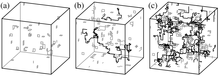
Figure 1: Samples of loop configurations for a $3d$ hypercubic lattice with side length $L\!=\!24$ and periodic boundary conditions. Percolating (nonpercolating) loops are colored black (gray). The snapshots relate to different values of the disorder parameter $\rho$, i.e. (a) $\rho\!=\!0.10$, (b) $\rho\!=\!0.13$, (c) $\rho\!=\!0.17$, so as to illustrate the NWP of loops. In the limit of large system sizes and above the critical point $\rho_{c}\!=\!0.1273(3)$, the lattice features system-spanning loops of total negative weight.

Here, we study the negative weight percolation problem on hypercubic lattice graphs in dimensions $d\!=\!2$ through $7$. The aim of the present study is to determine the upper critical dimension of the NWP problem from computer simulations for systems with finite size. In this regard, we compute the ground state (GS) loop configurations for the NWP model for a fairly general disorder distribution (described below in Sec. II) and characterize the resulting loops using observables from percolation theory. We perform finite-size scaling analyses to extrapolate the results to the thermodynamic limit. As a fundamental observable that provides information on whether the upper critical dimension $d_{u}$ is reached, we monitor the fractal dimension $d_{f}$ of the loops. The fractal dimension can be defined from the scaling of the average length $\langle\ell\rangle$ of the percolating loops as a function of system size $L$ according to $\langle\ell\rangle\!\sim\!L^{d_{f}}$. In $2d$ we previously obtained the estimate $d_{f}\!=\!1.266(2)$ Melchert and Hartmann (2008). This tells that in $2d$ the loops are, in a statistical sense, somewhat less convoluted than SAWs ($d_{f}^{\rm SAW}\!=\!1.333$). For $d\!\geq\!d_{u}$ we expect to observe $d_{f}\!=\!2$, as for usual self-avoiding lattice curves. This means, the “excluded volume” effect mentioned earlier becomes irrelevant and the loops exhibit the same scaling as ordinary random walks.

The remainder of the presented article is organized as follows. In section II, we introduce the model in more detail and we outline the algorithm used to compute the loop configurations. In section III, we list the results of our numerical simulations and in section IV we conclude with a summary.

II Model and Algorithm

In the remainder of this article we consider regular hypercubic lattice graphs $G\!=\!(V,E)$ with side length $L$ and fully periodic boundary conditions (BCs) in dimensions $d\!=\!2\ldots 7$. The considered graphs have $N\!=\!|V|\!=\!L^{d}$ sites $i\!\in\!V$ and a number of $|E|\!=\!dN$ undirected edges $\{i,j\}\!\in\!E$ that join adjacent sites $i,j\!\in\!V$. We further assign a weight $\omega_{ij}$ to each edge contained in $E$, representing quenched random variables that introduce disorder to the lattice. In the present work we consider lattices which exhibit a fraction $(1-\rho)$ of edges with weight 1 and a fraction $\rho$ of edges following a Gaussian disorder, i.e.,

$$P(\omega)=\rho\exp{(-\omega^{2}/2)}/\sqrt{2\pi}+(1-\rho)\delta(\omega-1)\,.$$ (1)

This allows explicitly for loops $\mathcal{L}$ with a negative total weight $\omega_{\mathcal{L}}\!=\!\sum_{\{i,j\}\in\mathcal{L}}\omega_{ij}$. To support intuition: For any nonzero value of the disorder parameter $\rho$, a sufficiently large lattice will exhibit at least “small” loops that have negative weight, see Fig. 1(a). If the disorder parameter is large enough, system-spanning loops with negative weight will exist, see Figs. 1(b),(c).

The NWP problem statement then reads as follows: Given $G$ together with a realization of the disorder, determine a set $\mathcal{C}$ of loops such that the configurational energy, defined as the sum of all the loop-weights $\mathcal{E}\!=\!\sum_{\mathcal{L}\in\mathcal{C}}\omega_{\mathcal{L}}$, is minimized. Therein, the weight of an individual loop is smaller than zero. As further optimization constraint, the loops are not allowed to intersect. Note that $\mathcal{C}$ may also be empty (clearly this is the case for $\rho\!=\!0$). The set of optimum loops is obtained using an appropriate transformation of the original graph as detailed in Ahuja et al. (1993). For the transformed graphs, minimum-weight perfect matchings (MWPM) Cook and Rohe (1999); Hartmann and Rieger (2001); Melchert (2009a) are calculated, yielding the loops for each particular instance of the disorder. This procedure allows for an efficient implementation Hartmann (2009) of the simulation algorithms. Here, we give a brief description of the algorithmic procedure that yields a minimum-weight set of loops for a given realization of the disorder. Fig. 2 illustrates the 3 basic steps, which are detailed next:

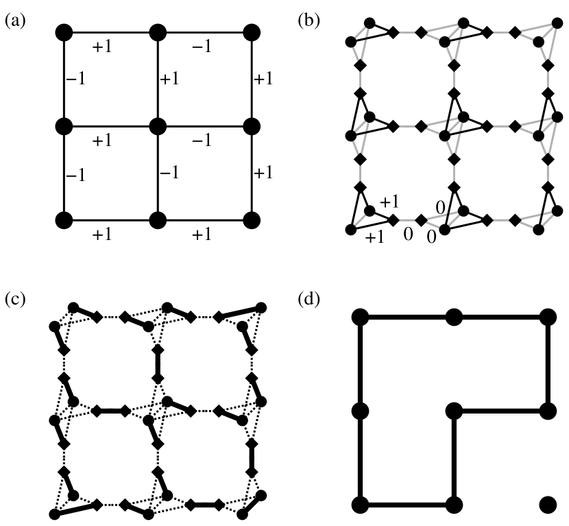
Figure 2: Illustration of the algorithmic procedure: (a) original lattice $G$ with edge weights, (b) auxiliary graph $G_{\rm A}$ with proper weight assignment. Black edges carry the same weight as the respective edge in the original graph and grey edges carry zero weight, (c) minimum-weight perfect matching (MWPM) $M$: bold edges are matched and dashed edges are unmatched, and (d) loop configuration (bold edges) that corresponds to the MWPM depicted in (c).

(1) each edge, joining adjacent sites on the original graph $G$, is replaced by a path of 3 edges. Therefore, 2 “additional” sites have to be introduced for each edge in $E$. Therein, one of the two edges connecting an additional site to an original site gets the same weight as the corresponding edge in $G$. The remaining two edges get zero weight. The original sites $i\in V$ are then “duplicated”, i.e. $i\rightarrow i_{1},i_{2}$, along with all their incident edges and the corresponding weights. For each of these pairs of duplicated sites, one additional edge $\{i_{1},i_{2}\}$ with zero weight is added that connects the two sites $i_{1}$ and $i_{2}$. The resulting auxiliary graph $G_{{\rm A}}=(V_{{\rm A}},E_{{\rm A}})$ is shown in Fig. 2(b), where additional sites appear as squares and duplicated sites as circles. Fig. 2(b) also illustrates the weight assignment on the transformed graph $G_{{\rm A}}$. Note that while the original graph (Fig. 2(a)) is symmetric, the transformed graph (Fig. 2(b)) is not. This is due to the details of the mapping procedure and the particular weight assignment we have chosen. A more extensive description of the mapping can be found in Melchert and Hartmann (2007).

(2) a MWPM on the auxiliary graph is determined via exact combinatorial optimization algorithms com . A MWPM is a minimum-weighted subset $M$ of $E_{\rm A}$, such that each site contained in $V_{\rm A}$ is met by precisely one edge in $M$. This is illustrated in Fig. 2(c), where the solid edges represent $M$ for the given weight assignment. The dashed edges are not matched. Due to construction, the auxiliary graph consists of an even number of sites and since there are no isolated sites, it is guaranteed that a perfect matching exists.
Note that obtaining the MWPM can be done in polynomial time as a function of the number of sites, hence large system sizes with hundreds of thousands of sites are feasible.

(3) finally it is possible to find a relation between the matched edges $M$ on $G_{\rm A}$ and a configuration of negative-weighted loops $\mathcal{C}$ on $G$ by tracing back the steps of the transformation (1). Regarding this, note that each edge contained in $M$ that connects an additional site (square) to a duplicated site (circle) corresponds to an edge on $G$ that is part of a loop, see Fig. 2(d). Note that, by construction of the auxiliary graph, for each site $i_{1}$ or $i_{2}$ matched in this way, the corresponding twin site $i_{2}$/$i_{1}$ must be matched to an additional site as well. This guarantees that wherever a path enters a site of the original graph, the paths also leaves the site, corresponding to the defining condition of loops. All the edges in $M$ that connect like sites (i.e. duplicated-duplicated, or additional-additional) carry zero weight and do not contribute to a loop on $G$. Once the set $\mathcal{C}$ of loops is found, a depth-first search Ahuja et al. (1993); Hartmann and Rieger (2001) can be used to identify the loop set $\mathcal{C}$ and to determine the geometric properties of the individual loops. For the weight assignment illustrated in Fig. 2(a), there is only one negative weighted loop with $\omega_{\mathcal{L}}\!=\!-2$ and length $\ell=8$.

Note that the result of the calculation is a collection $\mathcal{C}$ of loops such that the total loop weight, and consequently the configurational energy $\mathcal{E}$, is minimized. Hence, one obtains a global collective optimum of the system. Obviously, all loops that contribute to $\mathcal{C}$ possess a negative weight. Also note that the choice of the weight assignment in step (1) is not unique, i.e. there are different ways to choose a weight assignment that all result in equivalent sets of matched edges on the transformed lattice, corresponding to the minimum-weight collection of loops on the original lattice. Some of these weight assignments result in a more symmetric transformed graph, see e.g. Ahuja et al. (1993). However, this is only a technical issue that does not affect the resulting loop configuration. Albeit the transformed graph is not symmetric, the resulting graph (Fig. 2(d)) is again symmetric. The small $2d$ lattice graph with free BCs shown in Fig. 2 was chosen intentionally for illustration purposes. The algorithmic procedure extends to higher dimensions and fully periodic BCs in a straight-forward manner.

In the following section we will use the procedure outlined above to investigate the NWP phenomenon on hypercubic lattices.

III Results

In the current section we will present the results of our simulations, carried out in order to characterize the critical behavior of the NWP phenomenon in dimensions $d\!=\!2\ldots 7$. To accomplish this, we use observables similar to those used in percolation theory and perform FSS analyses. The fundamental observables related to an individual loop $\mathcal{L}$ are its weight $\omega_{\mathcal{L}}$ and length $\ell=\sum_{\{i,j\}\in\mathcal{L}}1$. Further, we determine the linear extensions $R_{i}$, $i\!=\!1\ldots d$, of a given loop by projecting it onto the independent lattice axes. The largest of those values, i.e. $R\!=\!\max_{i\!=\!1\ldots d}(R_{i})$, is referred to as the spanning length of the loop. To characterize the full perimeter of an individual loop on a coarse grained scale, we can further define the “size” $R_{s}\!=\!\sum_{i=1}^{d}R_{i}$, i.e. the length of the loop if all small scale irregularities where flattened Vachaspati and Vilenkin (1984). The remainder of the present section is organized as follows. In subsections III.1 and III.2, we will first locate the critical points and exponents that characterize the NWP phenomenon on hypercubic lattice graphs. Therefore we perform FSS analyses that involve data for different values of the disorder parameter. For these scaling analyses we considered hypercubic lattices with side lengths up to $L_{\rm max}$, and a respective number of disorder configurations $n_{\rm max}$, as listed in Tab. 1. In subsection III.3 we will then state our results on the critical behavior of energetic and geometric loop-observables. Therefore, right at the critical points for the various dimensions, we perform simulations for lattices up to $L_{\rm max}^{\rho_{c}}$ and $n_{\rm max}^{\rho_{c}}$, as listed in Tab. 1.

Table 1: System sizes and number of disorder configurations considered. From left to right: dimension $d$, largest system size $L_{\rm max}$ and respective number of samples $n_{\rm max}$ considered for the scaling analysis that involves various values of the disorder parameter $\rho$, largest system size $L_{\rm max}^{\rho_{c}}$ and number of samples $n_{\rm max}^{\rho_{c}}$ considered for the analysis at $\rho_{c}$, and, number $N_{\rm loops}$ of loops collected at $L_{\rm max}^{\rho_{c}}$.

$d$	$L_{\rm max}$	$n_{\rm max}$	$L_{\rm max}^{\rho_{c}}$	$n_{\rm max}^{\rho_{c}}$	$N_{\rm loops}$
$2$	$128$	$40\,000$	$512$ ($384$)	$3\,200$ ($21\,200$)	$25\,144\,685$
$3$	$48$	$9\,600$	$56$	$19\,200$	$14\,292\,489$
$4$	$24$	$4\,800$	$24$	$9\,600$	$4\,172\,813$
$5$	$12$	$6\,400$	$12$	$12\,200$	$1\,762\,955$
$6$	$8$	$6\,400$	$8$	$6\,400$	$520\,368$
$7$	$5$	$4\,800$	$5$	$12\,800$	$204\,459$

III.1 Scaling analyses to obtain critical points and exponents in $d\!=\!2\ldots 7$

In the present subsection, we illustrate the analysis for the simulated data on $3d$ hypercubic lattices in detail. Although we performed similar analyses for the remaining dimensions, we do not show figures for $d\!=\!2,4-7$ but include the final results in Tab. 2.

Table 2: Critical properties that characterize the NWP phenomenon in $d\!=\!2\ldots 7$. From left to right: Lattice dimension $d$, critical point $\rho_{c}$, critical exponent $\nu$ that describes the divergence of a typical length scale, order parameter exponent $\beta$, fluctuation exponent $\gamma$, fractal dimension $d_{f}$ at criticality and Fisher exponent $\tau$. Note that the figures for $d\!=\!2$ are taken from Ref. Melchert and Hartmann (2008).

$d$	$\rho_{c}$	$\nu$	$\beta$	$\gamma$	$d_{f}$	$\tau$
2	0.340(1)	1.49(7)	1.07(6)	0.77(7)	1.266(2)	2.59(3)
3	0.1273(3)	1.00(2)	1.54(5)	-0.09(3)	1.459(3)	3.07(1)
4	0.0640(2)	0.80(3)	1.91(11)	-0.66(5)	1.60(1)	3.55(2)
5	0.0385(2)	0.66(2)	2.10(12)	-1.06(7)	1.75(3)	3.86(3)
6	0.0265(2)	0.50(1)	1.92(6)	-0.99(3)	2.00(1)	4.00(2)
7	0.0198(1)	0.41(1)	–	–	2.08(8)	4.50(1)

As pointed out earlier, a loop is called percolating if its spanning length $R$ is equal to the system size $L$. This is a binary decision for each realization of the disorder and it is further used to obtain the percolation probability $P_{L}(\rho)$ for a lattice graph of a certain size $L$ at a given value of the disorder parameter $\rho$. According to scaling theory, one expects $P_{L}(\rho)$ to satisfy the scaling expression

$$\langle P_{L}(\rho)\rangle\sim f_{1}[(\rho-\rho_{c})L^{1/\nu}],$$ (2)

wherein $\langle\ldots\rangle$ denotes the disorder average and $\rho_{c}$ is the critical value of the disorder parameter above which system spanning loops first appear as $L\!\to\!\infty$. Further, $\nu$ is a critical exponent that describes the divergence of a typical length scale in the NWP problem as the critical point is approached. Finally, $f_{1}[\cdot]$ denotes an (unknown) universal scaling function. Eq. 2 implies that if one plots $P_{L}(\rho)$ as a function of the scaled variable $x\equiv(\rho-\rho_{c})L^{1/\nu}$ and if one adjusts $\rho_{c}$ and $\nu$ to their proper values, one should find a collapse of the data curves belonging to different values of $L$ onto a master curve. Note that above, $x$ constitutes a lowest order polynomial approximation to $f_{1}[x]$ regarding the disorder parameter $\rho$ around the critical point $\rho_{c}$. The resulting scaling plot for the data of $3d$ hypercubic lattices is shown in Fig. 3(a). Therein, considering Eq. 2, a best data collapse of the curves for $L\!\geq\!24$ yields the parameters $\rho_{c}\!=\!0.1273(3)$ and $\nu\!=\!1.00(2)$ ($S\!=\!1.02$), where the scaling analysis was restricted to the finite interval $dx\!=\![-0.2\!:\!0.4]$ enclosing the critical point on the rescaled $x$-axis. The value of $S$ measures the mean square deviation of the data points from the master curve in units of the standard error and thus provides information on how well the simulated data fits the scaling expression, see Refs. Houdayer and Hartmann (2004); Melchert (2009b). Here, the data collapse is considered to be good if the numerical value of $S\!\leq\!2$. Further, the quality $S$ of the data collapse and the resulting estimates for the critical parameters did not depend much on the size of the chosen interval $dx$. As an alternative, the maxima of the associated fluctuations, i.e. ${\rm var}(P_{L}(\rho))\!=\!\langle P_{L}(\rho)^{2}\rangle\!-\!\langle P_{L}(\rho)\rangle^{2}$, can be used to define system size dependent, “effective” critical points $\rho(L)$ Stauffer and Aharony (1994). These maxima are located at precisely those values of $\rho$ where $P_{L}(\rho)\!=\!1/2$, and just as $P_{L}(\rho)$ approaches a step function in the thermodynamic limit, $\rho(L)$ approaches $\rho_{c}$ as $L\!\to\!\infty$.

Figure 3: Results of the FSS analyses for the NWP problem on $3d$ hypercubic lattice graphs. (a) scaling plot of the percolation probability $P_{L}(\rho)$. The main plot shows the data collapse after rescaling the raw data according to Eq. 2. The inset at the bottom illustrates the unscaled data close to the critical point $\rho_{c}$. The inset on top shows the scaling of the effective critical points $\rho(L)$, obtained from the finite size fluctuations ${\rm var}(P_{L}(\rho))$. (b) scaling plot of the order parameter $P_{\infty}$. The main plot shows the data collapse after rescaling the raw data according to Eq. 3, and the inset shows the unscaled data.

In this regard, we expect the sequence of effective critical points to attain an asymptotic value as $\rho(L)\!=\!\rho_{c}+aL^{-1/\nu}$. First, we obtained the estimates of $\rho(L)$ by fitting a Gaussian function to the peaks of ${\rm var}(P_{L}(\rho))$. Applying the above scaling form to the data points thus obtained (see upper inset of Fig. 3(a)), then yields $\rho_{c}\!=\!0.1270(4)$ and $\nu\!=\!1.02(4)$ in agreement with the estimates reported earlier. Further, for each realization of the disorder we can compute the size of the smallest box that fits the largest loop on the lattice, i.e. $V_{\rm B}\!=\!\Pi_{i=1}^{d}R_{i}$. For the normalized box-size we observe the scaling behavior $\langle V_{\rm B}/L^{d}\rangle\!\sim\!f_{2}[(\rho-\rho_{c})L^{1/\nu}]$ (not shown), with scaling parameters $\rho_{c}\!=\!0.1273(2)$ and $\nu\!=\!0.99(4)$ ($S\!=\!1.00$). Since the analyses related to these three different observables conclude with scaling parameters that agree within the error bars, we are confident that the respective values of $\rho_{c}$ and $\nu$, listed in Tab. 2, properly describe the critical behavior of the NWP phenomenon on $3d$ hypercubic lattice graphs.

A second critical exponent is related to the scaling behavior of the order parameter $P_{\infty}\!=\!\ell/L^{d}$, which measures the probability that a site on the lattice graph belongs to the largest loop. Therein, $\ell$ refers to the length of the largest loop for each realization of the disorder. According to scaling theory one can expect $P_{\infty}$ to scale as

$$\langle P_{\infty}\rangle\sim L^{-\beta/\nu}f_{3}[(\rho-\rho_{c})L^{1/\nu}],$$ (3)

wherein $\beta$ signifies the order parameter exponent. Again, for the $3d$ data, a FSS analysis utilizing a collapse of the data curves for $L\!\geq\!24$ yields the estimate $\beta\!=\!1.54(5)$ ($S\!=\!1.24$). A scaling plot of the order parameter is presented in Fig. 3(b). Therein, the data collapse is best close to the critical point. So as to reduce the effect of the corrections to scaling off criticality, the scaling analysis was restricted to the finite interval $dx\!=\![-0.15\!:\!0.225]$ on the rescaled $x$-axis.

The corresponding estimates of $\rho_{c}$, $\nu$ and $\beta$ for hypercubic lattice graphs in $d\!=\!2,4-7$, resulting from similar FSS analyses, are listed in Tab. 2.

III.2 Scaling analysis of the loop-length ratio

During the simulations we recorded the energetic and geometric properties of the largest and $2$nd largest loops, with respective lengths $\ell_{1}$ and $\ell_{2}$, for each realization of the disorder. The average loop-length ratio $\langle\ell_{1}/\ell_{2}\rangle$ for these loops was found to satisfy the scaling expression

$$\langle\ell_{1}/\ell_{2}\rangle\sim f_{4}[(\rho-\rho_{c})L^{1/\nu}].$$ (4)

In order to assess the corresponding scaling behavior, we discarded samples that featured less than two loops (i.e. samples with $\ell_{2}\!=\!0$). A similar scaling for the cluster-size ratio was previously confirmed for usual random percolation da Silva et al. (2002). It stems from the fact that the largest and $2$nd largest clusters exhibit the same fractal dimension at the critical point. For usual percolation this issue was addressed earlier Jan et al. (1998). Further, we observed a similar scaling behavior in the context of an analysis of ferromagnetic spin domains at the $T\!=\!0$ spin glass to ferromagnet transition for the $2d$ random bond Ising model Melchert and Hartmann (2009).

Figure 4: Results of the FSS analysis of the loop length ratio $\langle\ell_{1}/\ell_{2}\rangle$ on $3d$ hypercubic lattice graphs. The main plot shows the data collapse after rescaling the simulated data according to Eq. 4 and the inset illustrates the unscaled data close to the critical point.

Regarding the data for hypercubic lattices of different dimensions $d$ and considering Eq. 4, we here yield the estimates

$$3d : \rho_{c}\!= 0.1274(3) \nu\!= 0.99(5) S\!= 0.87 [-0.45\!:\!0.45]$$

$$4d : 0.0641(4) 0.80(9) 0.69 [-0.30\!:\!0.35]$$

$$5d : 0.0382(4) 0.68(9) 0.57 [-0.75\!:\!0.35]$$

$$6d : 0.0262(1) 0.50(3) 0.73 [-0.13\!:\!0.28]$$

that agree with those obtained earlier in subsection III.1, listed in Tab. 2, within error bars. Note that for the $7d$ systems, our data did not allow for a decent analysis of the loop-length ratio. Also, there are no results listed for the $2d$ case. This is so, since at the time we performed the simulations for the $2d$ square systems, we did not write out the second largest loop length, explicitly. A scaling plot that illustrates the behavior of the loop length ratio for the $3d$ systems is presented as Fig. 4. Further, note that the estimates of the scaling parameters (for the various values of $d$) did not depend much on the size of the considered scaling interval. E.g., for the $3d$ systems considering $dx\!=\![-0.4:1.25]$, we obtained $\rho_{c}\!=\!0.1273(4)$ and $\nu\!=\!1.00(6)$ with the somewhat larger quality $S\!=\!0.97$.

Note that the scaling according to Eq. 4 was established empirically. So as to check whether that scaling assumption fits the data well, we allowed for a further free parameter, considering a scaling of the form $\langle\ell_{1}/\ell_{2}\rangle\!\sim\!L^{\kappa}f_{5}[(\rho-\rho_{c})L^{1/\nu}]$. We found that the best data collapse for given intervals $dx$ where attained for values $\rho_{c}$ and $\nu$ in agreement with those above and $|\kappa|\!\approx\!10^{-3}$.

III.3 Scaling at the critical point

As pointed out above, during the simulation we recorded the linear extensions $R_{i}$, $i\!=\!1\ldots d$, of the individual loops by projecting it onto the independent lattice axes. So as to study the scaling of the loop shape, we collected, for each dimension $d$, a large number $N_{\rm loops}$ of loops (see Tab. 1) at the critical point $\rho_{c}$ for the largest system size $L_{\rm max}^{\rho_{c}}$ considered for the respective setup. For those loops we then monitored the volume to surface ratio $V_{\rm B}/S_{\rm B}$ of the smallest box that fits the individual loops as a function of the coarse-grained loop size $R_{s}=\sum_{i=1}^{d}R_{i}$, where $V_{\rm B}\!=\!\Pi_{i=1}^{d}R_{i}$ and $S_{\rm B}\!=\!2\times\sum_{i=1}^{d}V_{\rm B}/R_{i}$. For hypercubic volumes with identical values $R_{i}$, $i\!=\!1\ldots d$, one would expect to find $V_{\rm B}/S_{\rm B}\!=\!(2dd)^{-1}R_{s}$. Considering $d\!=\!2\dots 6$ and performing fits to the form $\langle V_{\rm B}/S_{\rm B}\rangle_{R_{s}}\!=\!cR_{s}^{\psi}$ we yield $|\psi-1|\!\approx\!10^{-2}$ and values of $c$ reasonably close to $(2dd)^{-1}$ in order to conclude that the loops, in a statistical sense, are not oblate but possess a rather spherical shape. E.g., in $3d$ we obtained $c/(2dd)\!=\!0.95(1)$ and $\psi\!=\!1.00(3)$. However, in $7d$ the data is not well represented by the scaling form above. In this regard, we found our data best fit by the precise scaling form $\langle V_{\rm B}/S_{\rm B}\rangle_{\ell}\!=\!0.003(1)\!(\ell\!+\!15(3))^{1.1(1)}$, where we considered the “true” loop length $\ell$ instead of $R_{s}$. Unfortunately, this contains no information that relates to the “loop-shape factor” $(2dd)^{-1}$ introduced above.

Figure 5: Results of the FSS analyses to estimate the fractal dimension $d_{f}$ of the loops. The main plot shows the scaling of the average loop length $\langle\ell\rangle$ as function of the system size $L$ for $d\!=\!2\ldots 5$. The dashed lines indicate the asymptotic scaling according to $\langle\ell\rangle\!\sim\!L^{d_{f}}$, with values $d_{f}$ listed in Tab. 2. Note that the data sets where shifted upwards by a factor $4$, $20$ and $100$ for $d\!=\!3$, $4$, $5$, respectively. The inset shows the scaling of the average loop size $\langle R_{s}\rangle$ as function of the “true” loop length $\ell$ for $d\!=6,7$. The dashed lines are $\sim\!\ell^{1/2}$, to which the asymptotic scaling $\langle R_{s}\rangle\!\sim\!\ell^{1/d_{f}}$ can be compared. The $7d$ data was shifted upwards by a factor $2$.

Next, we aim to determine the fractal dimension $d_{f}$ of the loops, which can be defined from the scaling behavior of the average loop length $\langle\ell\rangle$ as a function of the linear extend $L$ of the hypercubic lattice graphs at the critical point $\rho_{c}$ according to $\langle\ell\rangle\!\sim\!L^{d_{f}}$. For dimensions $d\!=\!2\ldots 5$ we thus analyzed the largest loop found for each realization of the disorder and employed the scaling relation above, see Fig. 5. The resulting estimates for $d_{f}$ are listed in Tab. 2. Further, we verified that the probability density function $D_{L}(\rho)$ of the largest loop length found for each realization of the disorder yields a data collapse after a rescaling of the form $D_{L}(\ell)\!\sim\!L^{-d_{f}}f_{6}[\ell/L^{d_{f}}]$ (not shown). Due to the few and small system sizes that can be reached in $d\!=\!6$, $7$ ($L_{\rm max}^{\rho_{c}}\!=\!8,5$, respectively), the data analysis turned out to be somewhat more intricate. For those two cases we considered only the largest lattice and analyzed the scaling behavior of all the small, i.e. nonpercolating, loops, where we considered the scaling form $\langle R_{s}\rangle\!\sim\!\ell^{1/d_{f}}$. For the considered lattice sizes the values of $\ell$ where not too diverse and we collected $520368$ ($6d$) and $204459$ ($7d$) loops that comprise the estimates $d_{f}\!=\!2.00(1)$ ($6d$) and $2.08(8)$ ($7d$), see Fig. 5. However, note that for the data analysis all those data points have to be discarded that are strongly affected by the granularity of the lattice. For this reason, all the data points for $\ell\!\leq\!10$ have been withdrawn. Unfortunately, at $\rho_{c}$, the number density $n_{\ell}$ of loops with a given length $\ell$ decays algebraically as $n_{\ell}\!\sim\!\ell^{-\tau}$, where $\tau\!\geq\!1+d/2$ (see below). This means, considering $\ell\!>\!10$, the values of $d_{f}$ obtained from the scaling form above stem from only a fraction of the collected loops. E.g., for $6d$ and $\ell\!>\!10$ we have only $5884$ loops that represent the respective averages $\langle R_{s}\rangle$. Hence, the results for $d\!=\!6$ and $7$ have to be taken with a grain of salt. However, the fact that $d\!=\!6$ is the smallest dimension for which the fractal dimension of the loops attains the value of $d_{f}\!=\!2$ suggests an upper critical dimension $d_{u}\!=\!6$ for the NWP phenomenon. In a previous study Melchert and Hartmann (2008) we found that for $2d$ systems, the weight $\omega_{\mathcal{L}}$ of a loop $\mathcal{L}$ is proportional to its length $\ell$. Here, we verified the same behavior for the various dimensions considered. More precise, we collected loops for the largest system size $L_{\rm max}^{\rho_{c}}$ at the critical point $\rho_{c}$ of a given dimension $d$. Regarding the loop weight we found a best fit to the data by using the scaling form $\langle\omega_{\mathcal{L}}\rangle\!\sim\!\ell(1+c_{1}/\ell^{c_{2}})$, wherein $c_{1}$ was of order $10$ and $c_{2}\!\approx\!1$ for all dimensions considered.

Another critical exponent can be obtained from the scaling of the finite size susceptibility associated to the order parameter, i.e. $\chi_{L}\!=\!L^{d}{\rm var}(P_{\infty})\!\equiv\!L^{-d}{\rm var}(\ell)$. Basically, this observable measures the mean-square fluctuation of the loop length and it exhibits the critical scaling $\chi_{L}\!\sim\!L^{\gamma/\nu}$ (not shown). The resulting estimates of the fluctuation exponent $\gamma$ are listed in Tab. 2 and are found to agree with the scaling relation $\gamma+2\beta=d\nu$ within error bars. Note that in $7d$ the quality of the data was not sufficient to obtain an estimate for $\gamma$.

Finally, we investigate the number density $n_{\ell}$ of all nonpercolating loops with length $\ell$. Right at the critical point, it is expected to exhibit an algebraic scaling $n_{\ell}\!\sim\!\ell^{-\tau}$, governed by the Fisher exponent $\tau$. For the largest lattice graphs simulated for the various values of $d$, we obtain the estimates listed in Tab. 2, see also Fig. 6. For the corresponding data analyses, very small loops have to be neglected since they are affected by the granularity of the lattice and very large loops have to be withdrawn since they are affected by the lattice boundaries. From scaling, the Fisher exponent can be related to the fractal dimension via the scaling relation $\tau-1\!=\!d/d_{f}$. Note that the values of $\tau$ and $d_{f}$ listed in Tab. 2 where obtained independently and are found to agree with the latter scaling relation within error bars, in support of the estimate $d_{u}\!=\!6$ suggested above.

Figure 6: Results of the FSS analyses for the number density $n_{\ell}$ of all nonpercolating loops with length $\ell$ for $d\!=\!2\ldots 7$. Right at $\rho_{c}$, the number density exhibits an algebraic scaling $n_{\ell}\!\sim\!\ell^{-\tau}$, with $\tau$ listed in Tab. 2. Note that the the data sets for dimensions $d$ where scaled by a factor $10^{2(6-d)}$.

IV Conclusions

In the present study, we performed numerical simulations on hypercubic lattice graphs with “Gaussian-like” disorder in dimensions $d\!=\!2$ through $7$. The aim of the study was to identify the upper critical dimension of the NWP phenomenon. Therefore, we used a mapping of the NWP model to a combinatorial optimization problem that allows to obtain configurations of minimum weight loops by means of exact algorithms. We characterized the loops using observables from percolation theory and performed FSS analyses to estimate critical points and exponents that describe the disorder driven, geometric phase transition related to the NWP problem in the different dimensions.

Albeit the data analysis is notoriously difficult for large values of $d$, we find our results consistent with an upper critical dimension $d_{u}\!=\!6$ for the NWP model. This conclusion was based on the estimates of the fractal dimension of the loops, which, in $6d$ attains the value $d_{f}\!=\!2$ for the first time (bear in mind that $d_{f}\!=\!2$ indicates the scaling of a completely uncorrelated lattice curve). Further, in $6d$, the critical exponent $\nu\!=\!0.5$ that describes the divergence of a typical length scale in the NWP problem matches the value of $\nu$ for usual random percolation at the upper critical dimension Stauffer and Aharony (1994). According to our results, the FSS exponent $\nu$ still changes for $d\!>\!d_{u}$, which, at a first glance appears to be a little odd. However, this seems to be in agreement with the FSS for random percolation above six dimensions, where it was found that the corresponding exponent takes the value $3/d$ Aharony and Stauffer (1995). Moreover, the value $\nu\!=\!0.41(1)$ for the $7d$ systems found here is close to the percolation estimate $3/7\!\approx\!0.429$.

At this point, we would like to note that its tempting to perform simulations for the NWP problem on random graphs, where one has direct access to the mean field exponents that describe the transition. Since the upper critical dimension can be defined as the smallest dimension for which the critical exponents take their mean field values, such simulations could be used to provide further support for the result $d_{u}\!=\!6$ obtained here.

Note that rather similar results where found in the context of the optimal-path problem Schwartz et al. (1998), wherein one aims to minimize the largest weight along a single path, in contrast to minimizing the sum of weights of multiple loops, as above. Further, the optimal path problem can be mapped to the minimum-spanning tree problem Dobrin and Duxbury (2001) and to invasion percolation with trapping Barabási (1996). Regarding the optimal path problem in strong disorder Buldyrev et al. (2004), quite similar fractal scaling exponents can be observed: $d_{\rm opt}\!=\!1.222(3)$ ($2d$, Ref. Middleton (2000)), $1.44(1)$ ($3d$, Ref. Buldyrev et al. (2004)) and $1.59(2)$ ($4d$, Ref. Cieplak et al. (1996) wherein also the approximate scaling relation $d_{\rm opt}\!=\!(d+4)/5$ was hypothesized). The correspondence to invasion percolation with trapping further suggests an upper critical dimension $d^{\rm opt}_{u}\!=\!6$ Buldyrev et al. (2004) for the optimal path problem.

Finally, we will elaborate on the results for the $3d$ systems. In an earlier study Melchert and Hartmann (2008), we performed simulations for $3d$ hypercubic lattice graphs respecting a bimodal distribution ($\omega\!=\!\pm 1$) of the edge-weights. Therein, the most reliable results include the estimates $\nu\!=\!1.02(3)$, obtained from a FSS analysis of the percolation probability, and $d_{f}\!=\!1.43(2)$, obtained from the scaling of the “small” loops at the respective critical point. These values are reasonably close to those found here for the “Gaussian-like” disorder in order to conclude that the exponents in $3d$ are universal, i.e. they do not depend on minor details of the problem setup as, e.g., the disorder distribution. Further, the exponents $\nu$, $\beta$ and $d_{f}$ for the $3d$ setup found here are close by those that describe the disorder induced vortex loop percolation transition for the superconductor-to-normal transition in a $3d$ strongly screened vortex glass model Pfeiffer and Rieger (2002).