Heat transport in quantum spin chains: the relevance of integrability

Abstract

We investigate heat transport in various quantum spin chains, using the projector operator technique. We find that anomalous heat transport is linked not to the integrability of the Hamiltonian, but to whether it can be mapped to a model of non-interacting fermions. Our results also suggest how seemingly anomalous transport may occur at low temperatures in a much wider class of models.

Heat transport in quantum spin chains, in particular when is normal (diffusive) transport observed, is still not understood despite considerable effort.Review2007 ; Review_Drude ; Heidrich_XXZ ; Klumper_XXZ ; Shastry_OBC ; Saito_Kubo ; Heidrich_XXZB ; Zotos_Drude ; Shastry ; Ian ; Tomaz For example, it was conjectured that integrability leads to anomalous (ballistic) transport,Zotos_Drude but it was also argued that an integrable gaped XXZ chain has normal conductivity.Shastry Others have argued that only the spin conductivity is normal in this case, while the thermal conductivity is still anomalous.Tomaz A consensus on what are the necessary criteria for normal conductivity is still missing.

Most of the above workHeidrich_XXZ ; Klumper_XXZ ; Shastry_OBC ; Saito_Kubo ; Heidrich_XXZB ; Zotos_Drude ; Shastry ; Ian studied infinite and/or periodic chains, and used the Kubo formulaKubo ; Luttinger where finite/zero Drude weight signals anomalous/normal transport. For integrable systems, the Kubo formula always predicts anomalous heat transport. In fact, full integrability is not even necessary, all that is needed is commutation of the heat current operator with the total Hamiltonian.Klumper_XXZ Anomalous heat transport observed experimentally in systems described by integrable models, such as (Sr,Ca)₁₄Cu₂₄O₄₁, Sr₂CuO₃ and CuGeO₃,e1 ; e2 ; e3 seems to validate this result, although Ref. e4, finds normal transport in Sr₂CuO₃ at high temperatures.

The proof of the Kubo formula requires dealing with currents between the chain’s ends and the thermal baths it is connected to.notem For infinite systems, one may argue that such currents can be ignored, as they are a boundary effect. However, the terms describing the coupling to the baths lead to a non-vanishing commutator between the heat current operator and the total Hamiltonian, invalidating the main argument for anomalous transport. In other words, “integrability” of the chain connected to baths may be lost even if the isolated chain is integrable. This conclusion is supported by recent proofs of Kubo-type formulae for finite systems, based on phenomenological approaches such as the Fokker-Planck equation.openKubo These Kubo formulae have similar structure to the original one, however the dynamics is not defined only by Hamiltonian of the chain but also includes random variables mimicking the effects of coupling to the baths.

Here we investigate finite spin chains coupled to thermal baths, using the projector technique.KuboBook ; Saito_Projector ; Li ; Mahler_Projector There are many other similar studiesSaito_Projector ; Li ; Mahler_Projector ; MM ; Saito_MD_EPL ; Mahler_Local ; Michel_HAM ; Tomaz for various spin Hamiltonians, most of which would be integrable for a periodic, isolated chain (hereafter we call such models integrable). Results range from normal to anomalous transport, and there is no agreement on whether integrability is correlated or not with anomalous transport.

We propose a resolution for this question in this Rapid Communication. We find that integrability is not a sufficient condition for anomalous heat transport. We find anomalous transport at all temperatures only in models which can be mapped onto homogeneous non-interacting fermionic models. All other models we investigated exhibit normal heat transport, whether they are integrable or not (however, as discussed below, at low temperatures their heat transport may become anomalous in certain conditions). We therefore conjecture that the existence of such a mapping is the criterion determining anomalous transport, at least for finite-size systems.

We begin by briefly describing our calculation method, which is a direct generalization of the projection operator technique used to study the evolution towards equilibrium of a system coupled to a single bath.KuboBook The $N$-site chain of spins-${1\over 2}$ is described by the Hamiltonian:

$${\cal H}_{S}=\sum_{i=1}^{N-1}\left[J_{x}s_{i}^{x}s_{i+1}^{x}+J_{y}s_{i}^{y}s_{i+1}^{y}+J_{z}s_{i}^{z}s_{i+1}^{z}\right]-\vec{B}\sum_{i=1}^{N}\vec{s}_{i}$$

while the heat baths are collections of bosonic modes:

$${\cal H}_{B}=\sum_{k,\alpha}\omega_{k,\alpha}b^{{\dagger}}_{k,\alpha}b_{k,\alpha}$$

where $\alpha=R/L$ indexes the right/left-side baths and we set $\hbar=1,k_{B}=1$, and the lattice constant $a=1$. The system-baths coupling is taken as:

$$V=\lambda\sum_{k,\alpha}V^{(\alpha)}_{k}s_{i_{\alpha}}^{y}\otimes\left(b^{{\dagger}}_{k,\alpha}+b_{k,\alpha}\right)$$

where $i_{L}=1$ and $i_{R}=N$, i.e. the left (right) thermal bath is only coupled to the first (last) spin and can induce its spin-flipping. This is because we choose $\vec{B}\cdot\vec{e}_{y}=0$ while $|\vec{B}|$ is finite, meaning that spins primarily lie in the $x0z$ plane so that $s^{y}$ acts as a spin-flip operator.

The evolution of the total system is described by the Liouville-von Neumann equation for the total density matrix $\hat{\rho}_{T}$. If we are interested only in the properties of the central system, it is convenient to find an equation of motion for the reduced density matrix $\hat{\rho}_{S}=tr^{B}\left(\hat{\rho}_{T}\right)$ and solve it directly. This is achieved by using the projection operators, treating the system-bath coupling perturbationally to second order, and also by using a Markovian approximation.KuboBook ; Saito_Projector These approximations are reasonable: the system-baths coupling must be rather weak so that the properties of the chain are determined by its specific Hamiltonian, not by this coupling. The Markovian approximation is also justified, since we are interested only in the steady-state limit $t\rightarrow\infty$.

The resulting equation of motion for $\hat{\rho}_{S}\left(t\right)$ is:

$$\frac{\partial\hat{\rho}_{S}(t)}{\partial t}=-i[{\cal H}_{S},\hat{\rho}_{S}(t)]-\lambda^{2}\sum_{\alpha=L,R}\left(\left[s_{i_{\alpha}}^{y},\hat{m}_{\alpha}\hat{\rho}_{S}(t)\right]+h.c.\right)$$ (1)

where $\hat{m}_{\alpha}=s_{i_{\alpha}}^{y}\cdot\hat{\Sigma}_{\alpha}$. Here, $(\cdot)$ refers to the element-wise product of two matrices, $\langle n|\hat{a}\cdot\hat{b}|m\rangle=\langle n|\hat{a}|m\rangle\langle n|\hat{b}|m\rangle$. The bath matrices $\hat{\Sigma}_{L,R}$ are defined in terms of the eigenstates of the system’s Hamiltonian ${\cal H}_{S}|n\rangle=E_{n}|n\rangle$ as:

$$\hat{\Sigma}_{\alpha}=\pi\sum_{m,n}|m\rangle\langle n|\left[\Theta\left(\Omega_{mn}\right)n_{\alpha}\left(\Omega_{mn}\right)D_{\alpha}\left(\Omega_{mn}\right)|V^{(\alpha)}_{k_{mn}}|^{2}\right.$$

$$\left.+\Theta\left(\Omega_{nm}\right)\left(1+n_{\alpha}\left(\Omega_{nm}\right)\right)D_{\alpha}\left(\Omega_{nm}\right)|V^{(\alpha)}_{k_{nm}}|^{2}\right]$$

where $\Omega_{mn}=E_{m}-E_{n}=-\Omega_{nm}$ and $k_{mn}$ is defined by $\omega_{k_{mn},\alpha}=\Omega_{mn}$, i.e. a bath mode resonant with this transition. Furthermore, $\Theta(x)$ is the Heaviside function, $n_{\alpha}(\Omega)=\left[e^{\beta_{\alpha}\Omega}-1\right]^{-1}$ is the Bose-Einstein equilibrium distribution for the bosonic modes of energy $\Omega$ at the bath temperature $T_{\alpha}=1/\beta_{\alpha}$, and $D_{\alpha}(\Omega)$ is the bath’s density of states. The product $D_{\alpha}\left(\Omega_{mn}\right)|V^{(\alpha)}_{k_{mn}}|^{2}$ is the bath’s spectral density function. For simplicity, we take it to be a constant independent of $m$ and $n$.

The same equation of motion for $\hat{\rho}_{S}(t)$ was also derived in Refs. Saito_Projector, ; Mahler_Projector, ; Li, , where its steady-state solution was found via Runge-Kutta integration or by solving an eigenvalue problem. The latter comes about because the steady-state $\hat{\rho}_{\infty}$ is given by $0={\cal L}\hat{\rho}_{\infty}$, where ${\cal L}$ is the linear operator on the RHS of Eq. (1), so in matrix terms $\rho_{\infty}$ is the eigenvector corresponding to the zero eigenvalue of ${\cal L}$. Using the normalization $tr\hat{\rho}_{\infty}=1$, this eigenvalue problem can be replaced with solving a linear system of coupled equations, which makes it more efficient and allows us to analyze somewhat larger systems.

We rewrite ${\cal H}_{S}=\sum_{i=1}^{N-1}h_{i,i+1}+\sum_{i=1}^{N}h_{i}$, where $h_{i,i+1}$ is the exchange between nearest-neighbor spins and $h_{i}$ is the on-site coupling to the magnetic field. We can then define a local site Hamiltonian $h^{(S)}_{i}={1\over 2}h_{i-1,i}+h_{i}+{1\over 2}h_{i,i+1}$ (with $h_{0,1}=h_{N,N+1}=0$) and a local bond Hamiltonian $h^{(B)}_{i}={1\over 2}h_{i}+h_{i,i+1}+{1\over 2}h_{i+1}$ such that ${\cal H}_{S}=\sum_{i=1}^{N}h^{(S)}_{i}=\sum_{i=1}^{N-1}h^{(B)}_{i}$. The local site Hamiltonians can be used to derive the heat current operator from the continuity equation $\hat{j}_{i\rightarrow i+1}-\hat{j}_{i-1\rightarrow i}=\nabla\hat{j}=-\frac{\partial h^{(B)}_{i}}{\partial t}=-i\left[{\cal H}_{S},h^{(B)}_{i}\right]$. This results in $\hat{j}_{i\rightarrow i+1}=i\left[h^{(B)}_{i},h^{(B)}_{i+1}\right]$ for $i=1,\cdots,N-2$. As expected, in the steady state we find $\langle\hat{j}_{i\rightarrow i+1}\rangle=J$ to be independent of $i$.

Knowledge of the steady state heat current $J$, as such, is not enough to decide whether the transport is normal or not. Consider an analogy with charge transport in a metal connected to two biased leads. What shows if the transport is anomalous is the profile of the electric potential, not the value of the electric current. In anomalous transport (clean, non-interacting metal) all the voltage drop occurs at the ends of the sample, near the contacts. Away from these contact regions, electrons move ballistically and the electric potential is constant, implying zero intrinsic resistance. For a dirty metal, scattering takes place everywhere inside the sample and the electric potential decreases monotonically in between the contact regions, i.e. the sample has finite intrinsic resistivity.

In principle, the scaling of the current with the sample size, for a fixed effective bias, also reveals the type of transport: for anomalous transport, the current is independent of the sample size once its length exceeds the sum of the two contact regions, while for normal transport it decreases like inverse length. The problem is that one needs to fix the effective bias, i.e. the difference between the applied bias and that in the contact regions. Furthermore, since we can only study relatively short chains, the results of such scaling may be questionable.

It is therefore desirable to use the equivalent of the electric potential for heat transport and to calculate its profile along in order to determine the type of transport. This, of course, is the “local temperature”, which is a difficult quantity to define. One consistency condition for any definition is that if $T_{L}=T_{R}=T$, i.e. the system is in thermal equilibrium at $T$, then all local temperatures should equal $T$. We define local site temperatures $T_{i}$ which fulfill this condition in the following way. Since we know all eigenstates of ${\cal H}_{S}$, it is straightforward to calculate its equilibrium density matrix at a given $T$, $\hat{\rho}_{S}^{eq,T}={1\over Z}\sum_{n}e^{-\beta E_{n}}|n\rangle\langle n|$, where $Z=\sum_{n}e^{-\beta E_{n}}$. Let then $\langle h_{i}^{(S)}\rangle_{eq,T}=tr[\hat{\rho}_{S}^{eq,T}h_{i}^{(S)}]$. We define $T_{i}$ to be the solution of the equation: $\langle h_{i}^{(S)}\rangle_{eq,T_{i}}=tr[\hat{\rho}_{\infty}h_{i}^{(S)}]$. In other words, the steady-state value of the energy at that site equals the energy the site would have if the whole system was in equilibrium at $T_{i}$. Of course, we can also use other “local” operators such as $h_{i}^{(B)}$ to calculate a local bond temperature $T_{i+{1\over 2}}$. We find that when these definitions are meaningful, the results are in very good agreement no matter what “local” operator is used.

This type of definition of $T_{i}$ is meaningful only if a large magnetic field $B$ is applied. For small $B$, the expectation values $\langle h_{i}^{(S)}\rangle_{eq,T}$ are very weakly $T$-dependent, so that tiny numerical errors in the steady-state value can lead to huge variations in $T_{i}$. Addition of a large $B$ is needed to obtain $\langle h_{i}^{(S)}\rangle_{eq,T}$ which varies fast enough with $T$ for values of interest so that a meaningful $T_{i}$ can be extracted. Since we could not find a meaningful definition for $T_{i}$ when $\vec{B}\rightarrow 0$, we cannot investigate such cases. Note, however, that most integrable models remain integrable under addition of an external field $\vec{B}=B\hat{e}_{z}$.

In all of our calculations, we take $B_{z}=1$ and the exchange $J\sim 0.1$. Temperatures $T_{L/R}=T(1\pm\delta/2)$ should not be so large that the steady state is insensitive to the model or so small that only the ground-state is activated. Reasonable choices lie between $\min(J_{x},J_{y},J_{z})$ and $NB$, which are roughly the smallest, respectively the largest energy scales for an $N$-site spin chain.

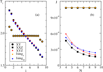
Figure 1: (color online) Plot of (a) local temperature profile for chains with $N=9$, and (b) thermal current $J$ vs. chain length $N$. In all cases $T_{L}=2.4,T_{R}=1.6$. Other non-zero parameters are $J_{x}=J_{y}=0.1,B_{z}=1$ (XY); $J_{x}=J_{y}={1\over 2}J_{z}=0.1,B_{z}=1$ (XXZ); $J_{x}={1\over 2}J_{y}={1\over 3}J_{z}=0.1,B_{z}=1$ (XYZ); $J_{z}=0.2,B_{x}=1$ (Ising_x) and $J_{z}=0.2,B_{x}=B_{z}=1$ (Ising_xz). The $XY$ and the Ising_x chains show flat $T_{i}$ profiles and currents independent of the chain’s length, i.e. anomalous transport. All other models have normal transport.

In Fig. 1(a) we show typical results for local temperature profiles $T_{i}$, $T_{i+{1\over 2}}$. We apply a large bias $\delta=(T_{L}-T_{R})/T=0.4$ for clarity, but we find similar results for smaller $\delta$ (see below). For these values, the “contact regions” include about two spins on either end. The $T_{i}$ profile of the rest of the chain is consistent with anomalous transport (flat $T_{i}$ profile) for the $XY$ chain and shows normal transport (roughly linear $T_{i}$ profile) in all the other non-Ising, $J_{z}\neq 0$ cases. We find similar results (not shown) for ferromagnetic couplings. All these are integrable models. The $XY$ model is special because it can be mapped to non-interacting spinless fermions with the Jordan-Wigner transformation.JW1 A finite $J_{z}$ leads to nearest-neighbor interactions between fermions. Eigenmodes for $J_{z}\neq 0$ can be found using Bethe’s ansatz, but they cannot be mapped to non-interacting fermions.

Another model that maps to non-interacting spinless fermions is the Ising model in a transverse field $B_{x}$.JW2 For this model we again find anomalous transport, as shown in Fig. 1(a). If we add a $B_{z}$ field, the model becomes non-integrablecomm2 and we recover normal transport. The scaling of $J$ vs. $N$, shown in Fig. 1(b), supports these conclusions, although a quantitative analysis is difficult because of the contact regions’s contributions.

We found this generic behavior for a wide range of parameters. When $\lambda\in\left[0.03,0.2\right]$, $T\in\left[0.3,30.0\right]$ and $\delta\geq 0.01$, the XYZ model has normal conductivity when $J_{z}\in\left[0.03,0.5\right]$ and anomalous conductivity when $J_{z}=0$. When $0<J_{z}<0.03$ or $J_{z}\in[0.5,1]$ the local temperature still decreases monotonically but not linearly, and the current decreases more slowly than $1/N$. Since we cannot study much longer chains we cannot easily distinguish here between normal vs. anomalous transport. For $J_{z}\geq 1$ the system becomes Ising-like and the transport is anomalous, as expected.

We would like to better gauge how things change with $N$, even with our limited range. For this, we consider how the effective temperature bias on the chain, $T_{2}-T_{N-1}$, or its effective slope $S=\frac{T_{2}-T_{N-1}}{N-3}$, depend on the system size $N$. For normal transport we expect $S\propto(N-\beta)^{-1}$ ($\beta$ accounts for the contact regions). If $S\propto(N-\beta)^{-\alpha}$ with $\alpha>1$, then for longer chains the temperature profile tends to be flatter than normal so we will use $\alpha>1$ as a signature of anomalous transport (of course, if a plateau starts to emerge near the center of chain that also indicates anomalous transport). A second gauge of the size dependence comes from looking at how the shape of the normalized temperature profile changes with $N$.

Figures 2(a) and (b) show such analysis. The left panel shows fits for $S$ (solid lines) for XXZ and XYZ models (symbols). Best fits give $\alpha<1$, consistent with normal transport. Similarly, the right panel which plots the normalized temperature profiles for different values of $N$ shows no change with increasing $N$, and no evidence that a plateau may evolve. Based on this limited evidence, we conclude that these models, although integrable, do exhibit normal transport.

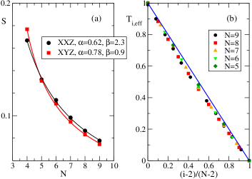
Figure 2: (a) Slope $S$ vs. system size $N$, and (b) normalized temperature $T_{i,{\rm eff}}=(T_{i}-T_{N-1})/(T_{2}-T_{N-1})$ for various systems sizes $N$. Parameters are $J_{x}=J_{y}=0.1$, $J_{z}=0.2$, $B_{z}=1.0$, $T=2.0$, $\delta=0.2$, $\lambda=0.1$. See text for more details.

In summary, the first conclusion we draw from these results is that integrability is not sufficient to guarantee anomalous transport: several integrable models show normal heat transport, in agreement with other studies.MM ; Mahler_Projector ; Michel_HAM ; Ian The second conclusion is that only models that map onto Hamiltonians of non-interacting fermions exhibit anomalous heat transport. This is a reasonable sufficient condition, since once inside the sample (past the contact regions) such fermions propagate ballistically. However, we cannot, at this stage, demonstrate that this is a necessary condition as well. We therefore can only conjecture that this is the criterion determining whether the heat transport is anomalous.

In this context, it is important to emphasize again the essential role played by the connection to the baths. In its absence, an isolated integrable model is described by Bethe ansatz type wavefunctions. Diffusion is impossible since the conservation of momentum and energy guarantees that, upon scattering, pairs of fermions either keep or interchange their momenta. For a system connected to baths, however, fermions are continuously exchanged with the baths, and the survival of a Bethe ansatz type of wavefunction becomes impossible. In fact, even the total momentum is no longer a good quantum number. We believe that this explains why normal transport in systems mapping to interacting fermions is plausible.

Normal transport is also possible for non-interacting fermions, if they are subject to elastic scattering on disorder. This can be realized, for example, by adding to the $XY$ model a random field $B_{z}$ at various sites. We have verified (not shown) that a local drop in the local temperature indeed arises near sites with such disorder, leading to normal conductance in “dirty” samples.

On the other hand, anomalous transport can also occur in models which map to homogeneous interacting fermions if the bath temperatures are very low. Specifically, consider the XXZ models. Because of the large $B_{z}$ we use, the ground-state of the isolated chain is ferromagnetic with all spins up. The first manifold of low-energy eigenstates have one spin flipped (single magnon states), followed by states with two spins flipped (two magnon states), etc. The separation between these manifolds is roughly $B_{z}$, although because of the exchange terms each manifold has a fairly considerable spread in energies and usually overlaps partially with other manifolds.

If both $T_{L},T_{R}\ll B_{z}$, only single-magnon states participate in the transport. We can then study numerically very long chains by assuming that the steady-state matrix elements $\rho_{nm}$ vanish for all other eigenstates ($S_{z,tot}$ is a good quantum number for these models). In this case we find anomalous transport for all models, whether integrable or not. This is reasonable, since the lone magnon (fermion) injected on the chain has nothing else to interact with, so it must propagate ballistically.

We can repeat this restricted calculation by including the two-magnon, three-magnon, etc. manifolds in the computation. As expected, the results agree at low $T_{L},T_{R}$, but differences appear for higher $T_{L},T_{R}$, when these higher-energy manifolds become thermally activated. In such cases, the transport becomes normal for the models mapping to interacting fermions as soon as the probability to be in the two (or more) magnon sector becomes finite. In other words, as soon as multiple excitations (fermions) are simultaneously on the chain, and inelastic scattering between them becomes possible.

These results may explain the heat transport observed experimentally in compounds such as Sr₂CuO₃,e4 where at low temperature anomalous transport was found while at high temperature normal transport was reported.

In conclusion, we propose a new conjecture for what determines the appearance of anomalous heat transport at all temperatures in spin chains. Unlike previous suggestions linking it to the integrability of the Hamiltonian or existence of gaps, we propose that the criterion is the mapping of the Hamiltonian onto a model of non-interacting fermions without any disorder.

Acknowledgments: Discussions and suggestions from Ian Affleck are gratefully acknowledged. Work supported by CIfAR Nanoelectronics, CFI and NSERC.

References

- (1) for a review, see A. V. Sologubenko et al., J. Low Temp. Phys. 147, 387 (2007)and references therein.
- (2) X. Zotos, J. Phys. Soc. Jpn. Suppl. 74, 173 (2005).
- (3) F. Heidrich-Meisner et al., Phys. Rev. B68, 134436 (2003).
- (4) A. Klümper and K. Sakai, J. Phys. A: Math. Gen. 35, 2173 (2002).
- (5) M. Rigol and B. S. Shastry, Phys. Rev. B77, 161101(R) (2008).
- (6) K. Saito, Phys. Rev. B 67, 064410 (2003).
- (7) F. Heidrich-Meisner et al., Phys. Rev. B71, 184415 (2005).
- (8) X. Zotos et al., Phys. Rev. B 55, 11029 (1997).
- (9) J. Sirker, R. G. Pereira and I. Affleck, Phys. Rev. Lett.103, 216602 (2009).
- (10) B. S. Shastry and B. Sutherland, Phys. Rev. Lett.65, 243 (1990).
- (11) T. Prosen and M. nidari, J. Stat. Mech. P02035 (2009).
- (12) R. Kubo, Journal of the Physical Society of Japan, 12, 570-586 (1957).
- (13) J.M. Luttinger, Phys. Rev. 135, A1505 (1964).
- (14) A. V. Sologubenko et al., Phys. Rev. Lett.84, 2714 (2000).
- (15) A. V. Sologubenko et al., Phys. Rev. B62, R6108 (2000).
- (16) Y. Ando et al., Phys. Rev. B58 R2913 (1998).
- (17) K. R. Thurberet al., Phys. Rev. Lett.87, 247202 (2001).
- (18) Thermal transport is driven by connecting the ends of the system to thermal baths, not by inducing a variation of the gravitational potential across the entire chain.
- (19) A. Kundu, A. Dhar and O. Narayan, J. Stat. Mech. L03001 (2009).
- (20) R. Kubo, M. Toda and N. Hashitsume, Statistical Physics II: Nonequilibrium Statistical Mechanics (Springer 1998).
- (21) K. Saito et al., Phys. Rev. E61, 2397 (2000).
- (22) Y. Yan, et al., Phys. Rev. B77, 172411(2008).
- (23) H. Weimer et al., Phys. Rev. E77, 011118 (2008).
- (24) M. Michel et al., Phys. Rev. B77, 104303 (2008).
- (25) K. Saito, Europhys. Lett.61, 34 (2003).
- (26) M. Michel et al., Phys. Rev. Lett.95, 180602 (2005).
- (27) M. Michel et al., Eur. Phys. B34, 325 (2003).
- (28) P. Jordan and E. Wigner, Z. Phys.47, 631 (1928).
- (29) R. V. Jensen and R. Shankar, Phys. Rev. Lett.54, 1879 (1985).
- (30) Similar results for the Ising chains in transverse field , with and without terms, have been reported in K. Saito et al., Phys. Rev. E54, 2404 (1996). There, however, the anomalous transport is assigned to integrability.