Fractional Chemotaxis Diffusion Equations.

Abstract

We introduce mesoscopic and macroscopic model equations of chemotaxis with anomalous subdiffusion for modelling chemically directed transport of biological organisms in changing chemical environments with diffusion hindered by traps or macro-molecular crowding. The mesoscopic models are formulated using Continuous Time Random Walk master equations and the macroscopic models are formulated with fractional order differential equations. Different models are proposed depending on the timing of the chemotactic forcing. Generalizations of the models to include linear reaction dynamics are also derived. Finally a Monte Carlo method for simulating anomalous subdiffusion with chemotaxis is introduced and simulation results are compared with numerical solutions of the model equations. The model equations developed here could be used to replace Keller-Segel type equations in biological systems with transport hindered by traps, macro-molecular crowding or other obstacles.

I Introduction

Diffusion and chemotaxis are fundamental to the motion of bacteria Wadhams and Armitage (2004), the directed motion of neutrophils in response to infection Van Haastert and Devreotes (2004), hypoxia stimulated angiogenesis Owen et al. (2009) and many other biological transport processes Van Haastert and Devreotes (2004). These transport processes can further be complicated by traps M.J. Saxton (2007), macromolecular crowding Dix and Verkman (2008) or other obstacles resulting in anomalous subdiffusion characterized by an ensemble averaged mean square displacement of diffusing species, $\langle r^{2}(t)\rangle$, that scales sublinearly in time, i.e., $\langle r^{2}(t)\rangle\sim t^{\gamma}$ with $0<\gamma<1$, R.N. Ghosh and W.W. Webb (1994); T.J. Feder et al. (1996); M.J. Saxton (1996); E.D. Sheets et al. (1997); P.R. Smith et al. (1999); E.B. Brown et al. (1999); Simson et al. (1998); Metzler and Klafter (2000); M.J. Saxton (2001); Weiss et al. (2003); D.S. Banks and Fradin (2005); Ozarslan et al. (2006). In this paper we introduce mesoscopic and macroscopic models for transport in biological systems with chemotaxis and anomalous subdiffusion.

The classic macroscopic model for the evolution of a diffusing species, with concentration $n(x,t)$, in the presence of a chemoattractant, with concentration $c(x,t)$, is the Keller-Segel model Keller and L.A. Segel (1971)

$$\frac{\partial n}{\partial t}=D\frac{\partial^{2}n}{dx^{2}}-\chi\frac{\partial}{\partial x}\left(n\frac{\partial c}{\partial x}\right)$$ (1)

where $D$ and $\chi$ denote the diffusion coefficient and the chemotactic coefficient respectively. In this model if the chemoattractant is removed the evolution corresponds to standard Brownian diffusion with $\langle r^{2}(t)\rangle\sim t$.

Anomalous subdiffusion can be modelled as fractional Brownian motion (fBm) Adelman (1976); K.G. Wang and C.W. Lung (1990); K.G. Wang et al. (1994) or Continuous Time Random Walks (CTRWs) Montroll and Weiss (1965); Scher and Lax (1973) with long-tailed waiting-time densities Metzler and Klafter (2000). Both of these models are non-Markovian and both exhibit the same sublinear scaling for the ensemble averaged mean square displacement. However the second moment of the velocity scales differently in the two models Lutz (2001) and the time averaged mean square displacement differs from the ensemble averaged mean square displacements in the CTRW model, but not in the fBm model He et al. (2008). Both possibilities should be considered when interpreting results from experiments using single particle tracking He et al. (2008) or fluorescence recovery after photobleaching Lubelski and Klafter (2008) and a simple test has been devised for analysing experimental data to determine which model is most appropriate Magdziarz et al. (2009).

At the macroscopic level, anomalous subdiffusion can be modelled through a modified diffusion equation

$$\frac{\partial C}{\partial t}={\mathcal{D}}(\gamma,t)\nabla^{2}C$$ (2)

with the diffusion constant replaced by a fractional temporal operator. In the case of fractional Brownian motion (fBm) this operator is given by K.G. Wang and C.W. Lung (1990); K.G. Wang et al. (1994)

$${\mathcal{D}}_{I}(\gamma,t)=D(\gamma)\gamma t^{\gamma-1}$$ (3)

In the Continuous Time Random Walk (CTRW) model Montroll and Weiss (1965), with power law waiting times Metzler and Klafter (2000), the fractional temporal operator is given by

$${\mathcal{D}}_{II}(\gamma,t)=D(\gamma)\frac{\partial^{1-\gamma}}{\partial t^{1-\gamma}}$$ (4)

where $D(\gamma)$ is a generalized diffusion coefficient with units of $m^{2}s^{-\gamma}$ and

$$\frac{\partial^{1-\gamma}}{\partial t^{1-\gamma}}Y(t)=\frac{1}{\Gamma(\gamma)}\frac{\partial}{\partial t}\int_{0}^{t}\frac{Y(t^{\prime})}{(t-t^{\prime})^{1-\gamma}}dt^{\prime}$$ (5)

defines the Riemann-Liouville fractional derivative of order $1-\gamma$. There have been various attempts to modify the fractional macroscopic equations to include force fields and reactions Metzler and Klafter (2000); B. I. Henry et al. (2010).

The Fokker-Planck equation for diffusion in a force field can readily be generalized by replacing the diffusion coefficient with a time dependent fractional operator as above. This has been justified within the framework of CTRWs, for force fields that vary in space but not time Barkai et al. (2000); Metzler and Klafter (2000) and for force fields that vary in time but not space I. M. Sokolov and Klafter (2006). However these derivations do not extend to the more general case of anomalous subdiffusion in a general external force field $f(x,t)$ that varies in both time and space. Two obvious possible generalizations in this case are I. M. Sokolov (2001)

$$\frac{\partial n}{\partial t}=\frac{\partial^{1-\gamma}}{\partial t^{1-\gamma}}D_{\gamma}\nabla^{2}n-\frac{1}{\eta_{\gamma}}\frac{\partial^{1-\gamma}}{\partial t^{1-\gamma}}\nabla\left(f(x,t)n(x,t)\right)$$ (6)

and Heinsalu et al. (2007); Weron et al. (2008); Heinsalu et al. (2009)

$$\frac{\partial n}{\partial t}=\frac{\partial^{1-\gamma}}{\partial t^{1-\gamma}}D_{\gamma}\nabla^{2}n-\frac{1}{\eta_{\gamma}}\nabla\left(f(x,t)\frac{\partial^{1-\gamma}}{\partial t^{1-\gamma}}n(x,t)\right).$$ (7)

If the force field is purely space dependent then the two models are equivalent and the solution is time subordinated to the concentration of diffusing species in the standard Fokker-Planck equation. This temporal subordination is not physically appropriate for time dependent external force fields Heinsalu et al. (2007). However an alternate formulation using an Ito stochastic differential equation has been proposed with a modified subordination in which the force varies in real time rather than the random time Weron et al. (2008). In chemotaxis there may be a physical link between the time scale of the diffusion and the time scale of the effective force field since the latter depends on the concentration of another diffusing species. Similarly in the fractional Nernst-Planck equation considered in B. I. Henry et al. (2008); T. A.M. Langlands et al. (2009) the force field from the membrane potential depends on concentrations of the diffusing species.

In Section II we introduce four different models of chemotaxis with anomalous subdiffusion. The different models are characterized by differences in the nature of the anomalous diffusion (fBm or power law CTRWs), and differences in the details of the underlying random walk processes. In Section III numerical solutions of the associated discrete space equations are obtained for each model. The numerical results are compared with Monte Carlo random walk simulations, with chemotactic forcing, on the same grid and using the same parameters. Differences between the model results are discussed in Section IV.

II Fractional Chemotaxis Diffusion Models

II.1 Model I

To model chemotaxis with fractional Brownian motion we consider an ad hoc model in which we replace both the diffusion coefficient and the chemotactic coefficient by fractional temporal operators as in Eq. (3). This yields

$$\frac{\partial n}{\partial t}=\gamma t^{\gamma-1}\left[D_{\gamma}\frac{\partial^{2}n}{\partial x^{2}}-\chi_{\gamma}\frac{\partial}{\partial x}\left(n\frac{\partial c}{\partial x}\right)\right]$$ (8)

where $\gamma$ is the anomalous diffusion exponent, $D_{\gamma}$ is the anomalous diffusion coefficient (with units $m^{2}s^{-\gamma}$), and $\chi_{\gamma}$ is the analogous anomalous chemotaxis coefficient. This model equation reduces to the standard Keller-Segel chemotaxis equation, Eq. (1), when $\gamma=1$.

II.2 Model II

A simple model for chemotaxis with fractional diffusion from power law CTRWs starts with the master equation

$$n_{i}(t)=n_{i}(0)\Phi(t)+\int\limits_{0}^{t}\left\{p_{r}(x_{i-1},t^{{}^{\prime}})n_{i-1}(t^{{}^{\prime}})+p_{l}(x_{i+1},t^{{}^{\prime}})n_{i+1}(t^{{}^{\prime}})\right\}\psi(t-t^{{}^{\prime}})\>dt^{{}^{\prime}}$$ (9)

where $\psi(t)$ is a (power law) waiting time density,

$$\Phi(t)=\int\limits_{t}^{\infty}\psi(t^{{}^{\prime}})\;dt^{{}^{\prime}}$$ (10)

is the corresponding survival probability, and $p_{r}(x,t)$ and $p_{l}(x,t)$ are the probabilities of jumping from $x$ to the adjacent grid point to the right and left directions respectively. These probabilities are dependent on the chemoattractant concentrations, $c(x,t)$, at the neighbouring points of the point $x$ at time $t$. The master equation, Eq. (9), is a continuous time representation of the transition probability law in Stevens (2000).

Following Stevens Stevens (2000), the probabilities of jumping to the left or right direction are based on the proportion of the chemoattractant on either side of the current point via

$$p_{l}(x_{i},t)=\frac{v(x_{i-1},t)}{v(x_{i-1},t)+v(x_{i+1},t)},$$ (11)

and

$$p_{r}(x_{i},t)=\frac{v(x_{i+1},t)}{v(x_{i-1},t)+v(x_{i+1},t)},$$ (12)

where $v(x,t)$ is a sensitivity function that depends on the concentration of the chemoattractant:

$$v(x,t)=\exp{\left(\beta\,c(x,t)\right)}.$$ (13)

Note that with the above we have

$$p_{l}(x_{i},t)+p_{r}(x_{i},t)=1$$ (14)

and

$$p_{l}(x_{i},t)-p_{r}(x_{i},t)=\frac{e^{\beta c(x_{i-1},t)}-e^{\beta c(x_{i+1},t)}}{e^{\beta c(x_{i-1},t)}+e^{\beta c(x_{i+1},t)}}.$$ (15)

Using the notation $\mathcal{L}\left\{f(t)\right\}\left(s\right)$ or $\widehat{f}(s)$ to denote the Laplace transform with respect to time of a function $f(t)$ we have the Laplace transform of Eq. (9),

$$\widehat{n}_{i}(s)=n_{i}(0)\widehat{\Phi}(s)+\left\{\mathcal{L}\left\{p_{r}(x_{i-1},t)n_{i-1}(t)\right\}\left(s\right)+\mathcal{L}\left\{p_{l}(x_{i+1},t)n_{i+1}(t)\right\}\left(s\right)\right\}\widehat{\psi}(s).$$ (16)

Using the identity

$$\widehat{\Phi}(s)=(1-\widehat{\psi}(s))/s,$$ (17)

which follows from the Laplace transform of (10), we have

$$s\widehat{n}_{i}(s)-n_{i}(0)=\frac{\widehat{\psi}(s)}{\widehat{\Phi}(s)}\left\{-\widehat{n}_{i}(s)+\mathcal{L}\left\{p_{r}(x_{i-1},t)n_{i-1}(t)\right\}\left(s\right)+\mathcal{L}\left\{p_{l}(x_{i+1},t)n_{i+1}(t)\right\}\left(s\right)\right\}.$$ (18)

We now consider a heavy-tailed waiting-time density which behaves for long-times as

$$\psi(t)\sim\frac{\kappa}{\tau}\left(\frac{t}{\tau}\right)^{-1-\gamma}$$ (19)

where $\gamma$ is the anomalous exponent, $\tau$ is the characteristic waiting-time, and $\kappa$ is a dimensionless constant. Using a Tauberian (Abelian) theorem Margolin (2004) we can write the Laplace transform for this density function as (for small $s$)

$$\widehat{\psi}(s)\sim 1-\frac{\kappa\Gamma\left(1-\gamma\right)}{\gamma}\left(s\tau\right)^{\gamma}.$$ (20)

Using Eq. (17), we then find the corresponding asymptotic form for the survival probability

$$\widehat{\Phi}(s)\sim\frac{\kappa\Gamma\left(1-\gamma\right)}{\gamma}\tau^{\gamma}s^{\gamma-1}$$ (21)

and the ratio

$$\frac{\widehat{\psi}(s)}{\widehat{\Phi}(s)}\sim A_{\gamma}\frac{s^{1-\gamma}}{\tau^{\gamma}}$$ (22)

where

$$A_{\gamma}=\frac{\gamma}{\kappa\Gamma\left(1-\gamma\right)}.$$

Specific cases of waiting time densities are the Mittag-Leffler density Scalas et al. (2003)

$$\psi(t)=-\frac{d}{dt}E_{\gamma}\left(-\left(\frac{t}{\tau}\right)^{\gamma}\right),$$ (23)

where $E_{\gamma}(z)$ is the Mittag-Leffler function Podlubny (1999), and the Pareto law used by S.B. Yuste et al. (2004)

$$\psi\left(t\right)=\frac{{\gamma}/{\tau}}{\left(1+t/\tau\right)^{1+\gamma}}.$$ (24)

The corresponding values for $A_{\gamma}$ can be shown to be

$$A_{\gamma}=1\quad\mathrm{and}\quad A_{\gamma}=\frac{1}{\Gamma\left(1-\gamma\right)}$$ (25)

for (23) and (24) respectively. Note the ratio in Eq.(22) is only valid long-times for the Pareto density, Eq. (24), whilst it is exact for the Mittag-Leffler density for all times. In addition, if $\gamma=1$ we do not use Eq. (24) but instead use Eq. (23).

With Eq. (22), Eq. (18) now becomes

$$s\widehat{n}_{i}(s)-n_{i}(0)=\frac{A_{\gamma}s^{1-\gamma}}{\tau^{\gamma}}\left\{-\widehat{n}_{i}(s)+\mathcal{L}\left\{p_{r}(x_{i-1},t)n_{i-1}(t)\right\}\left(s\right)+\mathcal{L}\left\{p_{l}(x_{i+1},t)n_{i+1}(t)\right\}\left(s\right)\right\}.$$ (26)

Noting that the Laplace Transform of a Riemann-Liouville fractional derivative of order $\alpha$, where $0<\alpha\leq 1$, is given by Podlubny (1999)

$$\mathcal{L}\left\{\frac{d^{\alpha}f(t)}{dt^{\alpha}}\right\}\left(s\right)=s^{\alpha}\widehat{f}(s)-\left[\frac{d^{\alpha-1}f(t)}{dt^{\alpha-1}}\right|_{t=0}$$ (27)

we can invert the Laplace transforms in Eq.(26) to obtain

$$\frac{dn_{i}}{dt}=\frac{A_{\gamma}}{\tau^{\gamma}}\frac{d^{1-\gamma}}{dt^{1-\gamma}}\left\{-n_{i}(t)+p_{r}(x_{i-1},t)n_{i-1}(t)+p_{l}(x_{i+1},t)n_{i+1}(t)\right\}$$ (28)

where we have ignored the last term in Eq. (27). Numerical solutions of this discrete space fractional differential equation for Model II are considered in Section III.

The spatial continuum limit of Model II can be obtained in the usual way by setting $x_{i}=x$ and $x_{i\pm 1}=x\pm\Delta x$ and carrying out Taylor series expansions in $x$. Retaining terms to order $(\Delta x)^{2}$ and using the normalization $p_{l}(x,t)+p_{r}(x,t)=1$ we first find that

$$-n_{i}(t)+p_{r}(x_{i-1},t)n_{i-1}(t)+p_{l}(x_{i+1},t)n_{i+1}(t) = \Delta x\frac{\partial}{\partial x}\left(n(x,t)[p_{l}(x,t)-p_{r}(x,t)]\right)$$ (29)

$$+\frac{\Delta x^{2}}{2}\frac{\partial^{2}}{\partial x^{2}}n(x,t).$$

This simplifies further after carrying out Taylor series expansions in Eq.(15), to arrive at

$$p_{l}(x,t)-p_{r}(x,t) \approx \frac{e^{-\beta\Delta x\frac{\partial c}{\partial x}}-e^{\beta\Delta x\frac{\partial c}{\partial x}}}{e^{-\beta\Delta x\frac{\partial c}{\partial x}}+e^{\beta\Delta x\frac{\partial c}{\partial x}}},$$ (30)

$$= -\tanh\left(\beta\Delta x\frac{\partial c}{\partial x}\right),$$

$$\approx -\beta\Delta x\frac{\partial c}{\partial x}.$$

We can now combine the results in Eq.(29) and Eq.(30) with Eq. (28) to obtain

$$\frac{\partial n}{\partial t}\simeq\frac{\partial^{1-\gamma}}{\partial t^{1-\gamma}}\left[\frac{A_{\gamma}\Delta x^{2}}{2\tau^{\gamma}}\frac{\partial^{2}n}{\partial x^{2}}(x,t)-\frac{A_{\gamma}\beta\Delta x^{2}}{\tau^{\gamma}}\frac{\partial}{\partial x}\left(\frac{\partial c(x,t)}{\partial x}n(x,t)\right)\right]+O(\Delta x^{4})$$ (31)

and then taking the limit $\Delta x\rightarrow 0$ and $\tau\rightarrow 0$, with

$$D_{\gamma}=\frac{A_{\gamma}\Delta x^{2}}{2\tau^{\gamma}}$$ (32)

and

$$\chi_{\gamma}=\frac{A_{\gamma}\beta\Delta x^{2}}{\tau^{\gamma}},$$ (33)

we have

$$\frac{\partial n}{\partial t}=\frac{\partial^{1-\gamma}}{\partial t^{1-\gamma}}\left[D_{\gamma}\frac{\partial^{2}n(x,t)}{\partial x^{2}}-\chi_{\gamma}\frac{\partial}{\partial x}\left(\frac{\partial c(x,t)}{\partial x}n(x,t)\right)\right].$$ (34)

Equation (34) provides a useful approximation for the space and time evolution of the concentration of an anomalously diffusing species that is chemotactically attracted by another species. In the CTRW master equation, Eq.(9) for this model the probabilities to jump left or right are determined at the start of the waiting times. We will consider another model in Section D where the probabilities to jump left or right are determined at the end of the waiting times. But first, in the next section, we consider an alternate formulation, based on a generalized master equation approach.

II.3 Model III

In this section we follow the generalised master equation approach of A.V. Chechkin et al. (2005); I. M. Sokolov and Klafter (2007, 2006), extended to take into account the effect of the chemoattractant. To begin we write the balance equation for the concentration of particles, $n$, at the site $i$

$$\frac{dn_{i}(t)}{dt}=J_{i}^{+}(t)-J_{i}^{-}(t),$$ (35)

where $J_{i}^{\pm}$ are the gain (+) and loss (-) fluxes at the site $i$. We also have the conservation equation for the arriving flux of particles at the point $i$ given by the flux of particles either leaving the site $i-1$ and jumping to the right or leaving the site $i+1$ that move to the left:

$$J_{i}^{+}(t)=p_{r}(x_{i-1},t)J_{i-1}^{-}(t)+p_{l}(x_{i+1},t)J_{i+1}^{-}(t)$$ (36)

where $p_{l}(x,t)$ and $p_{r}(x,t)$ are given in Eqs. (11) and (12). We can combine Eq. (36) and Eq.  (35) to obtain an evolution law for the concentration purely in terms of the loss flux, viz;

$$\frac{dn_{i}(t)}{dt}=p_{r}(x_{i-1},t)J_{i-1}^{-}(t)+p_{l}(x_{i+1},t)J_{i+1}^{-}(t)-J_{i}^{-}(t).$$ (37)

The loss flux at the site $i$ is given by

$$J_{i}^{-}(t)=\psi(t)n_{i}(0)+\int\limits_{0}^{t}\psi(t-t^{{}^{\prime}})J_{i}^{+}(t^{{}^{\prime}})\;dt^{{}^{\prime}}.$$ (38)

The first term represents those particles that were either originally at $i$ at $t=0$ and wait until time $t$ when they leave. The second term represents particles that arrived at some earlier time $t^{{}^{\prime}}$ and wait until time $t$ to leave. Here $\psi(t)$ is the usual waiting-time density used in Model II. We can combine Eq. (35) and Eq. (38) to obtain

$$J_{i}^{-}(t)=\psi(t)n_{i}(0)+\int\limits_{0}^{t}\psi(t-t^{{}^{\prime}})\left[J_{i}^{-}(t^{{}^{\prime}})+\frac{dn_{i}(t^{{}^{\prime}})}{dt}\right]\;dt^{{}^{\prime}}$$ (39)

and then we can solve for the loss flux using Laplace transform methods. The Laplace transform of Eq.(39) with respect to time yields

$$\widehat{J}_{i}^{-}(s)=\widehat{\psi}(s)n_{i}(0)+\widehat{\psi}(s)\left[\widehat{J}_{i}^{-}(s)+s\widehat{n}_{i}(s)-n_{i}(0)\right]$$ (40)

which simplifies further as

$$\widehat{J}_{i}^{-}(s)=\frac{\widehat{\psi}(s)}{\widehat{\phi}(s)}\widehat{n}_{i}(s).$$ (41)

Now using the approximation in Eq. (22) for a heavy-tailed waiting-time density and inverting the Laplace transform we have

$${J}_{i}^{-}(t)=\frac{A_{\gamma}}{\tau^{\gamma}}\frac{d^{1-\gamma}n_{i}(t)}{dt^{1-\gamma}}.$$ (42)

We now substitute the expression for the loss flux, Eq.(42) back into the balance equation, Eq.(37), to obtain

$$\frac{dn_{i}(t)}{dt}=\frac{A_{\gamma}}{\tau^{\gamma}}\left\{p_{r}(x_{i-1},t)\frac{d^{1-\gamma}n_{i-1}(t)}{dt^{1-\gamma}}+p_{l}(x_{i+1},t)\frac{d^{1-\gamma}n_{i+1}(t)}{dt^{1-\gamma}}-\frac{d^{1-\gamma}n_{i}(t)}{dt^{1-\gamma}}\right\}.$$ (43)

Numerical solutions of this discrete space fractional differential equation for Model III are considered in Section III.

The continuous space representation of Eq.(43) is found by setting $x_{i}=x$ and $x_{i\pm 1}=x\pm\Delta x$ so that

$$\frac{\partial n(x,t)}{\partial t}=\frac{A_{\gamma}}{\tau^{\gamma}}\left\{p_{r}(x-\Delta x,t)\frac{\partial^{1-\gamma}n(x-\Delta x,t)}{\partial t^{1-\gamma}}\right.\\ \left.+p_{l}(x+\Delta x,t)\frac{\partial^{1-\gamma}n(x+\Delta x,t)}{\partial t^{1-\gamma}}-\frac{\partial^{1-\gamma}n(x,t)}{\partial t^{1-\gamma}}\right\}.$$ (44)

The continuum limit representation can then be found by carrying out Taylor series expansions about $x$, similar to the steps used to reduce (28) to (34). This results in the equation

$$\frac{\partial n}{\partial t}=\frac{\partial^{1-\gamma}}{\partial t^{1-\gamma}}D_{\gamma}\frac{\partial^{2}n(x,t)}{\partial x^{2}}-\chi_{\gamma}\frac{\partial}{\partial x}\left(\frac{\partial c(x,t)}{\partial x}\frac{\partial^{1-\gamma}n(x,t)}{\partial t^{1-\gamma}}\right).$$ (45)

Model II and Model III are similar to the fractional Fokker Planck equations, Eq.(6) and Eq.(7) respectively with forcing from the chemotactic gradient $\frac{\partial c(x,t)}{\partial x}$.

II.4 Model IV

We now re-consider the master equation for the CTRW model but with the jump probabilities calculated after the particle has waited and immediately prior to jumping. The master equation in this case is given by

$$n_{i}(t)=n_{i}(0)\Phi(t)+p_{r}(x_{i-1},t)\int\limits_{0}^{t}n_{i-1}(t^{{}^{\prime}})\psi(t-t^{{}^{\prime}})\>dt^{{}^{\prime}}+p_{l}(x_{i+1},t)\int\limits_{0}^{t}n_{i+1}(t^{{}^{\prime}})\psi(t-t^{{}^{\prime}})\>dt^{{}^{\prime}}.$$ (46)

It is convenient to introduce the auxiliary function

$$m_{i}(t)=\int_{0}^{t}n_{i}(t^{{}^{\prime}})\psi(t-t^{{}^{\prime}})\>dt^{{}^{\prime}},$$ (47)

which has the Laplace transform

$$\widehat{m}_{i}(s)=\widehat{n}_{i}(s)\widehat{\psi}(s).$$ (48)

The Laplace transform of Eq.(46) with respect to time can then be written as

$$\left(s\widehat{n}_{i}(s)-n_{i}(0)\right)\widehat{\Phi}(s)=-\widehat{\psi}(s)\widehat{n}_{i}(s)+\mathcal{L}\left\{p_{r}(x_{i-1},t)m_{i-1}(t)\right\}\left(s\right)+\mathcal{L}\left\{p_{l}(x_{i+1},t)m_{i+1}(t)\right\}\left(s\right),$$ (49)

and after the inverse Laplace transform,

$$\int_{0}^{t}\frac{\partial n_{i}}{\partial t^{{}^{\prime}}}\Phi(t-t^{{}^{\prime}})\,dt^{{}^{\prime}}=m_{i}(t)+p_{r}(x_{i-1},t)m_{i-1}(t)+p_{l}(x_{i+1},t)m_{i+1}(t).$$ (50)

Proceeding to the continuum limit with Taylor series expansions about $x$, similar to the steps in Model II and Model III, we obtain

$$\int\limits_{0}^{t}\Phi(t-t^{{}^{\prime}})\frac{\partial n(x,t^{{}^{\prime}})}{\partial t}\>dt^{{}^{\prime}}\simeq\frac{\Delta x^{2}}{2}\frac{\partial^{2}m(x,t)}{\partial x^{2}}-\Delta{x}^{2}\beta\frac{\partial}{\partial x}\left(\frac{\partial c(x,t)}{\partial x}m(x,t)\right)+O(\Delta x^{4}),$$ (51)

and then using the auxiliary function definition in Eq.(47) we find

$$\int\limits_{0}^{t}\Phi(t-t^{{}^{\prime}})\frac{\partial n(x,t^{{}^{\prime}})}{\partial t}\>dt^{{}^{\prime}}\simeq\frac{\Delta x^{2}}{2}\int\limits_{0}^{t}\frac{\partial^{2}n(x,t^{{}^{\prime}})}{\partial x^{2}}\psi(t-t^{{}^{\prime}})\>dt^{{}^{\prime}}\\ -\Delta{x}^{2}\beta\frac{\partial}{\partial x}\left(\frac{\partial c(x,t)}{\partial x}\int\limits_{0}^{t}n(x,t^{{}^{\prime}})\psi(t-t^{{}^{\prime}})\>dt^{{}^{\prime}}\right)+O(\Delta x^{4}).$$ (52)

Asymptotic expressions for the convolution integrals in Eq.(52) can be obtained by considering asymptotic expansions in Laplace space and then inverting. Thus we now consider the terms

$$\mathcal{L}\left\{\int\limits_{0}^{t}\Phi(t-t^{{}^{\prime}})\frac{\partial n(x,t^{{}^{\prime}})}{\partial t}\>dt^{{}^{\prime}}\right\}\left(s\right) = \widehat{\Phi}(s)\mathcal{L}\left\{\frac{\partial n(x,t)}{\partial t}\right\}\left(s\right),$$ (53)

$$\mathcal{L}\left\{\int\limits_{0}^{t}\frac{\partial^{2}n(x,t^{{}^{\prime}})}{\partial x^{2}}\psi(t-t^{{}^{\prime}})\>dt^{{}^{\prime}}\right\}\left(s\right) = \widehat{\psi}(s)\frac{\partial^{2}\widehat{n}(x,s)}{\partial x^{2}},$$ (54)

$$\mathcal{L}\left\{\int\limits_{0}^{t}n(x,t^{{}^{\prime}})\psi(t-t^{{}^{\prime}})\>dt^{{}^{\prime}}\right\}\left(s\right) = \widehat{\psi}(s)\widehat{n}(x,s).$$ (55)

For long times (small $s$) we have, with the use of Eqs. (20) and (21)

$$\widehat{\Phi}(s) \simeq \frac{s^{\gamma-1}\tau^{\gamma}}{A_{\gamma}}+O(s^{2\gamma-1}),$$ (56)

$$\widehat{\psi}(s) \simeq 1-\frac{\left(s\tau\right)^{\gamma}}{A_{\gamma}}+O(s^{\gamma}).$$ (57)

Using these expansions in Eqs. (53) – (55) and taking the inverse Laplace transforms to replace the convolution integrals in Eq. (52) we obtain

$$\frac{\tau^{\gamma}}{A_{\gamma}}\frac{\partial^{\gamma-1}}{\partial t^{\gamma-1}}\frac{\partial n(x,t)}{\partial t}\simeq\frac{\Delta x^{2}}{2}\frac{\partial^{2}n(x,t)}{\partial x^{2}}-\Delta{x}^{2}\beta\frac{\partial}{\partial x}\left(\frac{\partial c(x,t)}{\partial x}n(x,t)\right)+O(\Delta x^{4}),$$ (58)

and in the limit $\Delta x\rightarrow 0$ and $\tau\rightarrow 0$

$$\frac{\partial n(x,t)}{\partial t}=\frac{\partial^{1-\gamma}}{\partial t^{1-\gamma}}\left[D_{\gamma}\frac{\partial^{2}n(x,t)}{\partial x^{2}}-\chi_{\gamma}\frac{\partial}{\partial x}\left(\frac{\partial c(x,t)}{\partial x}n(x,t)\right)\right]$$ (59)

as previously in Eq. (34).

Conversely, for short times (large $s$) we have

$$\widehat{\Phi}(s) \simeq \frac{1}{s}+O(s^{-\nu_{\gamma}-1}),$$ (60)

$$\widehat{\psi}(s) \simeq \frac{B_{\gamma}s^{-\nu_{\gamma}}}{\tau^{\nu_{\gamma}}}+O(s^{-2\nu_{\gamma}}),$$ (61)

where $\nu_{\gamma}=\gamma$ and $B_{\gamma}=1$ if use the Mittag-Leffler (23) and $\nu_{\gamma}=1$ and $B_{\gamma}=\gamma$ if we use the Pareto (24) density. The resulting equation for Eq. (52) becomes for short-times

$$\frac{\partial n(x,t)}{\partial t}=D^{*}_{\gamma}\frac{\partial^{1-\nu_{\gamma}}}{\partial t^{1-\nu_{\gamma}}}\frac{\partial^{2}n(x,t)}{\partial x^{2}}-\chi^{*}_{\gamma}\frac{\partial}{\partial x}\frac{\partial}{\partial t}\left(\frac{\partial c(x,t)}{\partial x}\frac{\partial^{-\nu_{\gamma}}n(x,t)}{\partial t^{-\nu_{\gamma}}}\right)$$ (62)

with the modified coefficients

$$D_{\gamma}^{*}=\frac{B_{\gamma}\Delta x^{2}}{2\tau^{\nu_{\gamma}}}$$ (63)

and

$$\chi_{\gamma}^{*}=\frac{B_{\gamma}\beta\Delta x^{2}}{\tau^{\nu_{\gamma}}}.$$ (64)

In the case of the Mittag-Leffler density (23), the short-time equation can be simplified to

$$\frac{\partial n(x,t)}{\partial t}=D_{\gamma}^{*}\frac{\partial^{1-\gamma}}{\partial t^{1-\gamma}}\frac{\partial^{2}n(x,t)}{\partial x^{2}}-\chi_{\gamma}\frac{\partial}{\partial x}\left(\frac{\partial c(x,t)}{\partial x}\frac{\partial^{1-\gamma}n(x,t)}{\partial t^{1-\gamma}}\right)\\ -\chi_{\gamma}^{*}\frac{\partial}{\partial x}\left(\frac{\partial^{2}c(x,t)}{\partial x\partial t}\frac{\partial^{-\gamma}n(x,t)}{\partial t^{-\gamma}}\right).$$ (65)

Equation (65) is similar to Model III’s governing equation given by Eq. (45) if we note that the last term which will be close to zero near $t=0$. Conversely if we use the Pareto density (24) then Eq. (62) becomes

$$\frac{\partial n(x,t)}{\partial t}=\gamma D_{1}\frac{\partial^{2}n(x,t)}{\partial x^{2}}-\gamma\chi_{1}\frac{\partial}{\partial x}\left(\frac{\partial c(x,t)}{\partial x}n(x,t)\right)\\ -\gamma\chi_{1}\frac{\partial}{\partial x}\left(\frac{\partial^{2}c(x,t)}{\partial x\partial t}\frac{\partial^{-1}n(x,t)}{\partial t^{-1}}\right)$$ (66)

which is similar to the standard chemotaxis equation (1) (if we again consider the last term to be small) except for the presence of the $\gamma$ term. This term will, in effect, slow the initial temporal behaviour of the solution (linear rescaling).

Note that if we use the Mittag-Leffler density in (23) then we see that the mesoscopic equation Eq. (46) bridges the gap between Model II and Model III. At short times it recovers Model III, Eq.(45), whereas at long times it recovers Model II (34). The latter shows that for long times, compared to the characteristic time $\tau$, there is no difference between evaluating the chemotactic probabilities at the time before or after the particle waits.

III Fractional Chemotaxis Reaction-Diffusion Models

In this section we consider extensions of the CTRW based fractional chemotaxis diffusion models to incorporate reactions. In the absence of chemotaxis, extensions of CTRW based fractional diffusion models to include linear reactions were derived in B. I. Henry et al. (2006); I.M. Sokolov et al. (2006) and extensions to include nonlinear reactions were derived in Yadav and Horsthemke (2006); Fedotov (2010).

III.1 Model II

Following the approach in B. I. Henry et al. (2006) we can incorporate reactions in CTRW models by increasing or decreasing the concentration of particles during the waiting times by an amount proportional to the evolution operator for the reaction dynamics. The master equation for Model II with linear reaction dynamics incorporated in this way becomes

$$n_{i}(t)=e^{kt}n_{i}(0)\Phi(t)+\int\limits_{0}^{t}\left\{p_{r}(x_{i-1},t^{{}^{\prime}})n_{i-1}(t^{{}^{\prime}})+p_{l}(x_{i+1},t^{{}^{\prime}})n_{i+1}(t^{{}^{\prime}})\right\}e^{k\left(t-t^{{}^{\prime}}\right)}\psi(t-t^{{}^{\prime}})\>dt^{{}^{\prime}}$$ (67)

where $k$ is the per capita rate gain ($k>0$) or loss ($k<0$) of particles. Again Laplace transform methods can be used to convert the integral equation representation into a (fractional) differential equation. The Laplace transform of Eq. (67) with respect to time yields

$$\widehat{n}_{i}(s)=n_{i}(0)\widehat{\Phi}(s-k)+\mathcal{L}\left\{p_{r}(x_{i-1},t)n_{i-1}(t)\right\}\left(s\right)\widehat{\psi}(s-k)\\ +\mathcal{L}\left\{p_{l}(x_{i+1},t)n_{i+1}(t)\right\}\left(s\right)\widehat{\psi}(s-k),$$ (68)

and after rearranging we find

$$s\widehat{n}_{i}(s)-n_{i}(0)=k\widehat{n}_{i}(s)+\frac{\widehat{\psi}(s-k)}{\widehat{\Phi}(s-k)}\left\{-\widehat{n}_{i}(s)+\mathcal{L}\left\{p_{r}(x_{i-1},t)n_{i-1}(t)\right\}\left(s\right)\right.\\ \left.+\mathcal{L}\left\{p_{l}(x_{i+1},t)n_{i+1}(t)\right\}\left(s\right)\right\},$$ (69)

where we have used (17). With the result in Eq.(22) we can inverting the Laplace transform to obtain

$$\frac{dn_{i}}{dt}=e^{kt}\frac{A_{\gamma}}{\tau^{\gamma}}\frac{d^{1-\gamma}}{dt^{1-\gamma}}\left(e^{-kt}\left[-n_{i}(t)+p_{r}(x_{i-1},t)n_{i-1}(t)+p_{l}(x_{i+1},t)n_{i+1}(t)\right]\right)+kn_{i}(t)$$ (70)

where the Riemann-Liouville fractional derivative has been replaced by a modified fractional derivative B. I. Henry et al. (2006); I.M. Sokolov et al. (2006).

The continuum limit, found by taking Taylor series expansions about $x$, is

$$\frac{\partial n}{\partial t}=e^{kt}\frac{\partial^{1-\gamma}}{\partial t^{1-\gamma}}\left(e^{-kt}\left[D_{\gamma}\frac{\partial^{2}n(x,t)}{\partial x^{2}}-\chi_{\gamma}\frac{\partial}{\partial x}\left(\frac{\partial c(x,t)}{\partial x}n(x,t)\right)\right]\right)+kn(x,t).$$ (71)

We note if $n(x,t)$ is not self-chemotactic then the solution of (71) is given by $n(x,t)=e^{kt}y(x,t)$ where $y(x,t)$ is the solution of (34) with $y$ replacing $n$.

III.2 Model III

To incorporate reactions in Model III we start by modifying Eq. (35) to

$$\frac{dn_{i}(t)}{dt}=J_{i}^{+}(t)-J_{i}^{-}(t)+kn_{i}(t)$$ (72)

where $k$, again, is the per capita rate gain ($k>0$) or loss ($k<0$) of particles. We also modify the expression for the loss flux, $J_{i}^{-}(t)$, in (38) to

$$J_{i}^{-}(t)=e^{kt}\psi(t)n_{i}(0)+\int\limits_{0}^{t}e^{k\left(t-t^{{}^{\prime}}\right)}\psi(t-t^{{}^{\prime}})J_{i}^{+}(t^{{}^{\prime}})\;dt^{{}^{\prime}}$$ (73)

where the exponential factors take into account the per capita addition or removal of particles as in B. I. Henry et al. (2006).

Now solving for the gain flux, $J^{+}_{i}(t)$, in Eq. (72) we find

$$J_{i}^{+}(t)=J_{i}^{-}(t)+\frac{dn_{i}(t)}{dt}-kn_{i}(t)$$ (74)

and using Eq. (73) gives

$$J_{i}^{-}(t)=e^{kt}\psi(t)n_{i}(0)+\int\limits_{0}^{t}e^{k\left(t-t^{{}^{\prime}}\right)}\psi(t-t^{{}^{\prime}})\left[J_{i}^{-}(t^{{}^{\prime}})+\frac{dn_{i}(t^{{}^{\prime}})}{dt}-kn_{i}(t^{{}^{\prime}})\right]\;dt^{{}^{\prime}}.$$ (75)

Now using Laplace transform theory we find

$$\widehat{J}_{i}^{-}(s)=\widehat{\psi}(s-k)n_{i}(0)+\widehat{\psi}(s-k)\left[\widehat{J}_{i}^{-}(s)+s\widehat{n}_{i}(s)-n_{i}(0)-k\widehat{n}_{i}(s)\right]$$ (76)

and upon solving for the flux, we find a similar expression to Eq. (41),

$$\widehat{J}_{i}^{-}(s)=\frac{\widehat{\psi}(s-k)}{\widehat{\Phi}(s-k)}\widehat{n}_{i}(s).$$ (77)

This Laplace trasnform can now be inverted to find the loss flux given by the modified fractional derivative B. I. Henry et al. (2006); I.M. Sokolov et al. (2006) of the concentration at $i$,

$${J}_{i}^{-}(t)=e^{kt}\frac{A_{\gamma}}{\tau^{\gamma}}\frac{d^{1-\gamma}}{dt^{1-\gamma}}\left(e^{-kt}n_{i}(t)\right),$$ (78)

where $A_{\gamma}$ is a constant given by $1$ or $1/\Gamma\left(1-\gamma\right)$ if we use the waiting-time density in Eq. (23) or Eq. (24) respectively.

Now using (36) and (78) in (72) we find

$$\frac{dn_{i}(t)}{dt}=p_{r}(x_{i-1},t)e^{kt}\frac{A_{\gamma}}{\tau^{\gamma}}\frac{d^{1-\gamma}}{dt^{1-\gamma}}\left(e^{-kt}n_{i-1}(t)\right)+p_{l}(x_{i+1},t)e^{kt}\frac{A_{\gamma}}{\tau^{\gamma}}\frac{d^{1-\gamma}}{dt^{1-\gamma}}\left(e^{-kt}n_{i+1}(t)\right)\\ -e^{kt}\frac{A_{\gamma}}{\tau^{\gamma}}\frac{d^{1-\gamma}}{dt^{1-\gamma}}\left(e^{-kt}n_{i}(t)\right)+kn_{i}(t).$$ (79)

The continuum limit following from setting $x_{i}=x$, $x_{i\pm 1}=x\pm\Delta x$, and Taylor series expansions about $x$, is given by

$$\frac{\partial n}{\partial t}=D_{\gamma}e^{kt}\frac{\partial^{1-\gamma}}{\partial t^{1-\gamma}}\left(e^{-kt}\frac{\partial^{2}n(x,t)}{\partial x^{2}}\right)-\chi_{\gamma}\frac{\partial}{\partial x}\left(\frac{\partial c(x,t)}{\partial x}e^{kt}\frac{\partial^{1-\gamma}}{\partial t^{1-\gamma}}\left(e^{-kt}n(x,t)\right)\right)+kn(x,t).$$ (80)

III.3 Model IV

The master equation for Model IV, Eq.(46), modified to include linear reaction dynamics is given by

$$n_{i}(t)=e^{kt}n_{i}(0)\Phi(t)+p_{r}(x_{i-1},t)\int\limits_{0}^{t}n_{i-1}(t^{{}^{\prime}})e^{k\left(t-t^{{}^{\prime}}\right)}\psi(t-t^{{}^{\prime}})\>dt^{{}^{\prime}}\\ +p_{l}(x_{i+1},t)\int\limits_{0}^{t}n_{i+1}(t^{{}^{\prime}})e^{k\left(t-t^{{}^{\prime}}\right)}\psi(t-t^{{}^{\prime}})\>dt^{{}^{\prime}}.$$ (81)

Following similar steps used to simplify Eq. (46) and using Taylor series expansions we find

$$\int\limits_{0}^{t}e^{k\left(t-t^{{}^{\prime}}\right)}\Phi(t-t^{{}^{\prime}})\frac{\partial n(x,t^{{}^{\prime}})}{\partial t}\>dt^{{}^{\prime}}\simeq\frac{\Delta x^{2}}{2}\int\limits_{0}^{t}\frac{\partial^{2}n(x,t^{{}^{\prime}})}{\partial x^{2}}e^{k\left(t-t^{{}^{\prime}}\right)}\psi(t-t^{{}^{\prime}})\>dt^{{}^{\prime}}\\ +k\int\limits_{0}^{t}e^{k\left(t-t^{{}^{\prime}}\right)}\Phi(t-t^{{}^{\prime}})n(x,t^{{}^{\prime}})\>dt^{{}^{\prime}}-\Delta{x}^{2}\beta\frac{\partial}{\partial x}\left(\frac{\partial c(x,t)}{\partial x}\int\limits_{0}^{t}n(x,t^{{}^{\prime}})e^{k\left(t-t^{{}^{\prime}}\right)}\psi(t-t^{{}^{\prime}})\>dt^{{}^{\prime}}\right)+O(\Delta x^{4}).$$ (82)

Using Laplace transforms and the asymptotic expressions in Eqs. (56) and (57) (evaluated for $s-k$ small) we arrive at Eq. (71) for long times.

For short times we find

$$\frac{\partial n(x,t)}{\partial t}=D^{*}_{\gamma}e^{kt}\frac{\partial^{1-\nu_{\gamma}}}{\partial t^{1-\nu_{\gamma}}}\left(e^{-kt}\frac{\partial^{2}n(x,t)}{\partial x^{2}}\right)-\chi^{*}_{\gamma}e^{kt}\frac{\partial}{\partial x}\frac{\partial}{\partial t}\left(\frac{\partial c(x,t)}{\partial x}\frac{\partial^{-\nu_{\gamma}}}{\partial t^{-\nu_{\gamma}}}\left(e^{-kt}n(x,t)\right)\right)+kn(x,t)$$ (83)

with $\nu_{\gamma}$ and the modified coefficients as defined previously for Model IV in section II.

IV Numerical Solutions and Monte Carlo Simulations

It is straightforward to obtain numerical solutions of the above model equations using difference approximations. In this section we describe numerical solutions for self-chemotactic variants of the model equations and we compare the solutions with Monte Carlo simulations.

Implementation details for the Monte Carlo simulations are described in the Appendix A. In the results reported here simulations were conducted on a one-dimensional lattice using the Pareto waiting-time density (24) with the characteristic waiting-time $\tau=0.1$, fractional exponent $\gamma=0.5$, and chemotactic sensitivity, $\beta$. The simulation results are from an average of 200 runs with 10, 000 particles initially located at the origin.

As our starting point for numerical solutions of the macroscopic models we consider the discrete space variants of Model II, III, and IV given by Eq (28), (43), and  (46) respectively. A discrete space variant for Model I, analogous to the discrete space variant for Model II, is given by

$$\frac{dn_{i}(t)}{dt}=\frac{A_{\gamma}\gamma t^{\gamma-1}}{\tau^{\gamma}}\left[p_{r}(x_{i-1},x_{i},t)n_{i-1}(t)+p_{l}(x_{i+1},x_{i},t)n_{i+1}(t)-n_{i}(t)\right]$$ (84)

The discrete space equations for Models II and III were solved using an implicit time stepping method with the fractional derivatives approximated using the L1 scheme Oldham and Spanier (1974) as in T.A.M. Langlands and B.I. Henry (2005). For Model IV, the integrals in the discrete space representation were approximated by taking the unknown concentration, $n_{i\pm 1}(t)$, to be piecewise linear in time.

The numerical solutions of the discrete space equations and the Monte Carlo simulations were performed using the same space grid size and similar values for the parameters $\tau$, $\gamma$, and $\beta$. We also chose the same initial condition (one at the origin and zero elsewhere). The constant $A_{\gamma}$ was chosen as in Eq. (25) since we used the Pareto density, Eq. (24), in the simulations.

In Figure 1 we compare the Monte Carlo simulation results with the numerical solution of the discrete space equations for each model with the chemotactic sensitivity parameter, $\beta=0.1$. Further results are shown in Figures 2 and 3 for the sensitivity parameter values $\beta=1$ and $\beta=10$ respectively.

The numerical solutions for Model III Eq (43) and Model IV (46) are in close agreement with the Monte Carlo simulations at all times. The numerical solution for Model II does not fit with the Monte Carlo simulations well at short times but it provides a good fit at long times ($t=20$). The numerical solution for Model I does not fit the Monte Carlo simulations well, especially for small values of $\beta$, where the predicted shape near the origin is smoother than that exhibited by the simulation data.

The closer agreement between the numerical results for Models III and IV and the Monte Carlo simulations is due to the timing of the chemotactic forcing. In models III and IV, and in the Monte Carlo simulations the chemotactically influenced jumping probabilities are determined at the end of the waiting times, whereas in Model II they are determined at the start of the waiting times. This difference is less marked if the chemotactic concentration varies slowly in time.

Overall, the numerical solutions for Model III provide better agreement with the Monte Carlo simulations than the numerical solutions for Model IV. This better agreement can be seen at the intermediate value of $\beta=1$ in Figure 2. This better agreement may be due to differences in numerical errors in approximating the discrete space equations for Model II and Model IV rather than due to differences between the equations themselves.

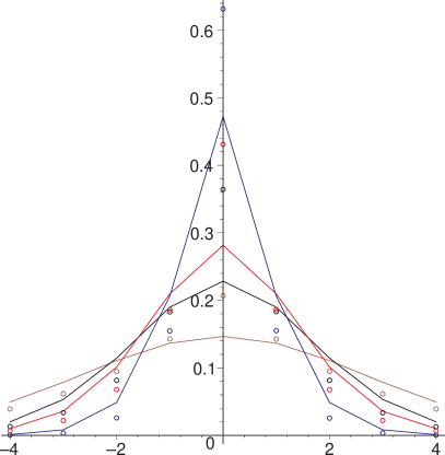
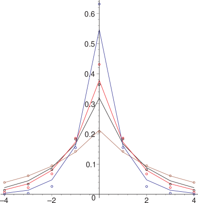
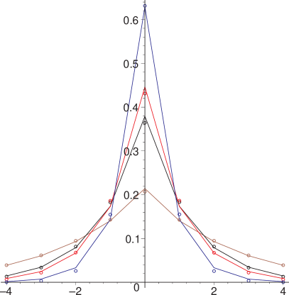
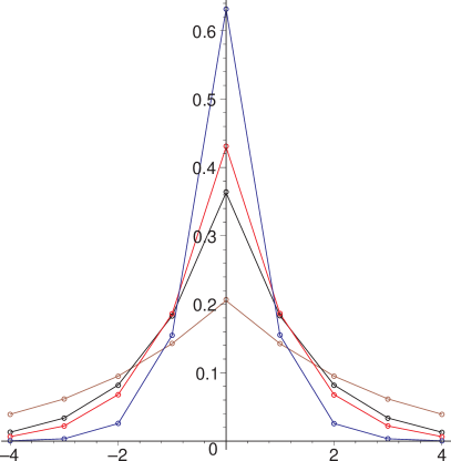
Figure 1: One-dimensional subdiffusive chemotaxis simulation results (circles) with $\beta=0.1$ showing the concentration profile at $t=0.4$ (blue), $t=2$ (red), $t=4$ (black), and $t=20$ (brown) compared with the numerical solution of the governing equations for models I (top left), II (top right), III (bottom left) and IV (bottom right) (solid lines).

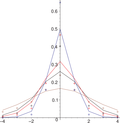
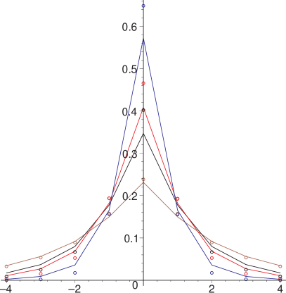
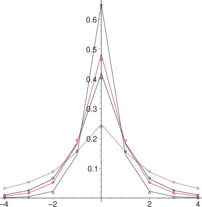
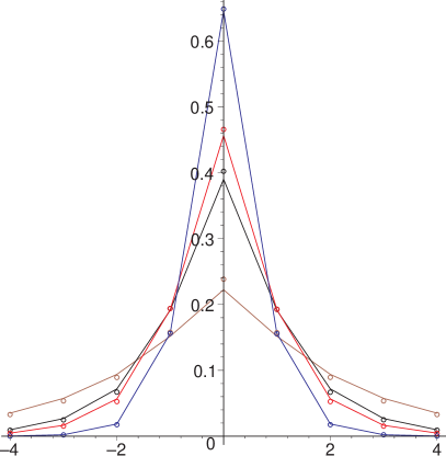
Figure 2: One-dimensional subdiffusive chemotaxis simulation results (circles) with $\beta=1.0$ showing the concentration profile at $t=0.4$ (blue), $t=2$ (red), $t=4$ (black), and $t=20$ (brown) compared with the numerical solution of the governing equations for models I (top left), II (top right), III (bottom left) and IV (bottom right) (solid lines).

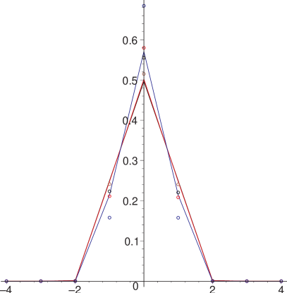
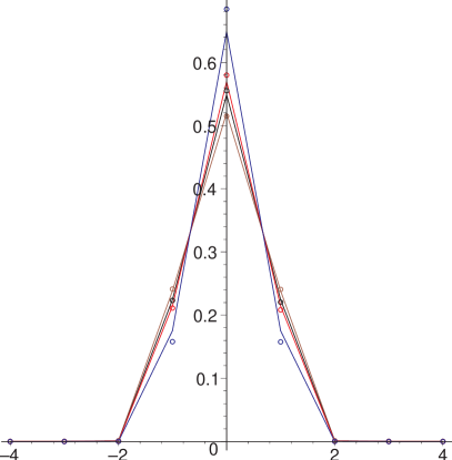
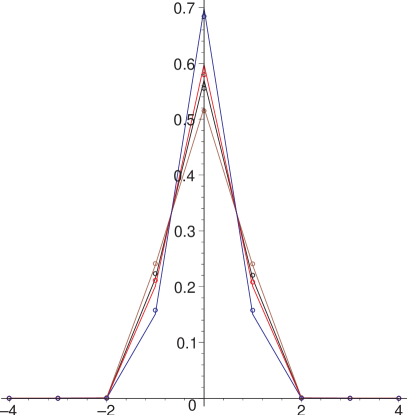
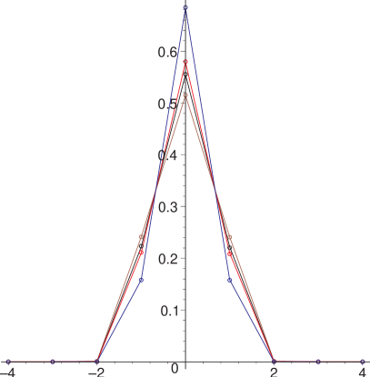
Figure 3: One-dimensional subdiffusive chemotaxis simulation results (circles) with $\beta=10.0$ showing the concentration profile at $t=0.4$ (blue), $t=2$ (red), $t=4$ (black), and $t=20$ (brown) compared with the numerical solution of the governing equations for models I (top left), II (top right), III (bottom left) and IV (bottom right) (solid lines).

V Summary and Discussion

The correct form of the fractional Fokker-Planck for particles undergoing anomalous subdiffusion in an external space and time varying force field has been an open problem. In the absence of a force field, subdiffusion can be modelled with a fractional temporal derivative operating on the spatial Laplacian. For subdiffusion in a purely space dependent force field the fractional temporal derivative can be put to the left of the standard terms on the right hand side of the standard Fokker-Planck equation Metzler et al. (1999); Barkai et al. (2000); Metzler and Klafter (2000); I. M. Sokolov (2001) as in Eq.(6). However the consensus has been that for subdiffusion in an external space-time-dependent force field the fractional temporal derivative should not operate on the force field Heinsalu et al. (2007); Weron et al. (2008); Heinsalu et al. (2009), as in Eq.(7). The modelling is further complicated if the force itself is affected directly or indirectly by the subdiffusing particles. This is the case in fractional electro-diffusion and fractional chemotaxis diffusion, the case considered here.

In this article we have introduced and investigated four models for particles undergoing anomalous subdiffusion in the presence of chemotactic forcing. The first being based on an adhoc extension to the fractional Brownian motion equation (Model I), two models based on Continuous Time Random Walk (CTRW) master equations where concentration-dependent jump probabilities were evaluated before (Model II) or after (Model IV) the particle waiting, and a fourth model derived from a generalized master equation (Model III). Concentration-dependent jump probabilities were used to incorporate the effect of chemotaxis in discrete space representations of the models and in the Monte Carlo (MC) simulations.

Evaluating the jump probabilities prior to waiting in the CTRW formulation (Model II) resulted in a macroscopic equation (valid in the long time limit) with the fractional derivative acting upon the chemotactic gradient. Conversely, using a generalized master equation approach with the probabilities evaluated after waiting but prior to jumping gave a macroscopic equation where the fractional derivative does not act upon the gradient (Model III). The CTRW formulation with the jump probabilities evaluated after waiting (Model IV) could only be reduced to a Fractional Fokker-Planck continuum equation in the asymptotic limit for long and short times. For long-times Models II and IV coincide whilst for short-times we found Models III and IV coincide asymptotically if a Mittag-Leffler density is used.

We also introduced Monte Carlo methods for simulating anomalous sub-diffusion in a chemotactic force field. In the Monte Carlo simulations the chemotactically influenced jump lengths were computed at the end of the waiting times, similar to Models III and IV. This could explain the excellent agreement we found between numerical solutions for Models III and IV and the Monte Carlo simulations. The numerical solutions for Model II also showed good agreement at long times. The numerical solutions based on the fractional Brownian motion equation, did not agree well with the Monte Carlo results.

The fractional chemotaxis diffusion models were further generalized to incorporate linear reaction dynamics. As in previous research, B. I. Henry et al. (2006); T. A.M. Langlands et al. (2008); I.M. Sokolov et al. (2006) we found that the incorporation of linear reactions required the replacement of the Riemann Liouville fractional derivative with a modified version, in addition to including the linear reaction term.

The fractional chemotaxis diffusion equations developed in this paper provide a new class of models for biological transport influenced by chemotactic forcing, macro-molecular crowding and traps. We have recently generalized these models to include arbitrary space-and-time dependent forces B.I. Henry et al. (2010).

Appendix A Monte Carlo Simulations

In this section we briefly describe the Monte Carlo method used to simulate chemotaxis on a periodic one-dimensional lattice with long-tailed waiting-time density (subdiffusion). For each simulation run, the following steps are conducted

1. Set the number of grid points, simulation time, and the initial number of particles.

2. Initialise the parameters for the waiting-time and jump-length probability density functions.

3. Set up the initial particle positions.

4. For each particle generate a random waiting-time, $\delta t$, (time of the first jump).

5. Initialise the output time $t_{out}=\Delta{t}$.

6. Find the time of the next jump by finding the minimum of all jumping times, $t_{jump}$.

7. If $t_{jump}>t_{out}$ then go to step (8) otherwise go to step (9).

8. Store the current particle positions. Add $\Delta{t}$ to $t_{out}$. If $t_{out}$ exceeds the simulation time then simulation ends otherwise go to step (7).

9. Generate a random jump-length, $\delta{x}$ (see below).

10. Generate a new waiting time and update this particle’s jumping time and position ($t_{jump}=t_{jump}+\delta{t}$ $x_{new}=x_{old}+\delta{x}$ ).

11. Go to step (6)

A.1 Generation of Waiting Times

The waiting times for each particle/jumper were generated by comparing a uniform random number, $r\in(0,1)$, with the cumulative probability function of the waiting-time density. We use the Pareto density (24) as the density which has used by Yuste, Acedo, and Lindeberg S.B. Yuste et al. (2004). The generated waiting-time is given as

$$\delta t=\tau\left(\left(1-r\right)^{-\frac{1}{\gamma}}-1\right)$$ (85)

where $r\in(0,1)$ is a uniform random number.

A.2 Generation of Jump Distances

The jump distance for each particle/jumper is generated by comparing an uniform random number, $r\in(0,1)$, with the cumulative probability function of the jump-length density.

For the simulations we use the jump-length probability density nearest neighbour jumps only:

$$\delta x=\left\{\begin{array}[]{cl}-\Delta{x},&\>0\leq r<p_{l},\\ \Delta{x},&\>p_{l}\leq r<1\end{array}\right.$$ (86)

where $\Delta x$ is the grid spacing and $p_{l}=p_{l}(x_{i},t)$ is the probability of jumping to the left given previously in Eqs. (11) and (13).

To evaluate the probabilities of jumping to the left or right for Eq. (86), requires the approximation of the chemoattractant concentration, $c(x_{i},t)$, in Eq. (13). This is estimated by the proportion of chemoattractant particles at the grid point, $x_{i}$, compared with the total number of particles in the system.

References

• Wadhams and Armitage (2004) G. Wadhams and J. Armitage, Nature Reviews: Molecular Cell Biology 5, 1024 (2004).
• Van Haastert and Devreotes (2004) P. Van Haastert and P. Devreotes, Nature Reviews, Molecular Cell Biology 5, 626 (2004).
• Owen et al. (2009) M. Owen, T. Alarcon, P. Maini, and H. Byrne, J. Math. Biol. 58, 689 (2009).
• M.J. Saxton (2007) M.J. Saxton, Biophys. J. 92, 1178 (2007).
• Dix and Verkman (2008) J. Dix and A. Verkman, Annu. Rev. Biophys. 37, 247 (2008).
• R.N. Ghosh and W.W. Webb (1994) R.N. Ghosh and W.W. Webb, Biophys. J. 66, 1301 (1994).
• T.J. Feder et al. (1996) T.J. Feder, I. Brust-Mascher, J.P. Slattery, B. Baird, and W.W. Webb, Biophys. J. 70, 2767 (1996).
• M.J. Saxton (1996) M.J. Saxton, Biophys. J. 70, 1250 (1996).
• E.D. Sheets et al. (1997) E.D. Sheets, G.M. Lee, R. Simson, and K. Jacobson, Biochem. 36, 12449 (1997).
• P.R. Smith et al. (1999) P.R. Smith, I.E.G. Morrison, K.M. Wilson, N. Fernandez, and R.J. Cherry, Biophys. J. 76, 3331 (1999).
• E.B. Brown et al. (1999) E.B. Brown, E.S. Wu, W. Zipfel, and W.W. Webb, Biophys. J. 77, 2837 (1999).
• Simson et al. (1998) R. Simson, B. Yang, S.E. Moore, P. Doherty, F.S. Walsh, and K.A. Jacobson, Biophys. J. 74, 297 (1998).
• Metzler and Klafter (2000) R. Metzler and J. Klafter, Phys. Rep. 339, 1 (2000).
• M.J. Saxton (2001) M.J. Saxton, Biophys. J. 81, 2226 (2001).
• Weiss et al. (2003) M. Weiss, H. Hashimoto, and T. Nilsson, Biophys. J 84, 4043 (2003).
• D.S. Banks and Fradin (2005) D.S. Banks and C. Fradin, Biophys. J 89, 2960 (2005).
• Ozarslan et al. (2006) E. Ozarslan, P. J. Basser, T. M. Shepherd, P. E. Thelwall, B. C. Vemuri, and S. J. Blackband, J. Magnetic Resonance 183, 315 (2006).
• Keller and L.A. Segel (1971) E. Keller and L.A. Segel, J. Theor. Biol. 30, 225 (1971).
• Adelman (1976) S. Adelman, J. Chem. Phys. 64, 124 (1976).
• K.G. Wang and C.W. Lung (1990) K.G. Wang and C.W. Lung, Physics Letters A 151, 119 (1990).
• K.G. Wang et al. (1994) K.G. Wang, L.K. Dong, X.F. Wu, F.W. Zhu, and T. Ko, Physica A 203, 53 (1994).
• Montroll and Weiss (1965) E. Montroll and G. Weiss, J. Math. Phys. 6, 167 (1965).
• Scher and Lax (1973) H. Scher and M. Lax, Phys. Rev. B. 7, 4491 (1973).
• Lutz (2001) E. Lutz, Physical Review E 64, 051106 (2001).
• He et al. (2008) Y. He, S. Burov, R. Metzler, and E. Barkai, Physical Review Letters 101, 058101 (2008).
• Lubelski and Klafter (2008) A. Lubelski and J. Klafter, Biophysical Journal 94, 4646 (2008).
• Magdziarz et al. (2009) M. Magdziarz, A. Weron, K. Burnecki, and J. Klafter, Physical Review Letters 103, 180602 (2009).
• B. I. Henry et al. (2010) B. I. Henry, T. A.M. Langlands, and P. Straka, in Complex Physical, Biophysical and Econophysical Systems: World Scientific Lecture Notes in Complex Systems, edited by R. L. Dewar and F. Detering (World Scientific, Singapore, 2010), vol. 9, pp. 37–90.
• Barkai et al. (2000) E. Barkai, R. Metzler, and J. Klafter, Phys. Rev. E 61, 132 (2000).
• I. M. Sokolov and Klafter (2006) I. M. Sokolov and J. Klafter, Phys. Rev. Lett. 97, 140602 (2006).
• I. M. Sokolov (2001) I. M. Sokolov, Phys. Rev. E 63, 056111 (2001).
• Heinsalu et al. (2007) E. Heinsalu, M. Patriarca, I. Goychuk, and P. Hänggi, Phys. Rev. Lett. 99, 120602 (2007).
• Weron et al. (2008) A. Weron, M. Magdziarz, and K. Weron, Phys. Rev. E 77, 036704 (2008).
• Heinsalu et al. (2009) E. Heinsalu, M. Patriarca, I. Goychuk, and P. Hänggi, Phys. Rev. E 79, 041137 (2009).
• B. I. Henry et al. (2008) B. I. Henry, T. A.M. Langlands, and S. L. Wearne, Phys. Rev. Lett. 100, 128103 (2008).
• T. A.M. Langlands et al. (2009) T. A.M. Langlands, B. I. Henry, and S. L. Wearne, J. Math. Biol 59, 761 (2009).
• Stevens (2000) A. Stevens, SIAM Journal on Applied Mathematics 61, 172 (2000).
• Margolin (2004) G. Margolin, Physica A 334, 46 (2004).
• Scalas et al. (2003) E. Scalas, R. Gorenflo, F. Mainardi, and M. Raberto, Fractals 11, 281 (2003).
• Podlubny (1999) I. Podlubny, Fractional differential equations, vol. 198 of Mathematics in Science and Engineering (Academic Press, New York and London, 1999).
• S.B. Yuste et al. (2004) S.B. Yuste, L. Acedo, and K. Lindenberg, Phys. Rev. E 69, 036126 (2004).
• A.V. Chechkin et al. (2005) A.V. Chechkin, R. Gorenflo, and I.M. Sokolov, J. Phys. A: Math. Gen. 38, L679 (2005).
• I. M. Sokolov and Klafter (2007) I. M. Sokolov and J. Klafter, Chaos, Solitons and Fractals 34, 81 (2007).
• B. I. Henry et al. (2006) B. I. Henry, T. A.M. Langlands, and S. L. Wearne, Phys. Rev. E 74, 031116 (2006).
• I.M. Sokolov et al. (2006) I.M. Sokolov, M.G.W. Schmidt, and F. Sagués, Phys. Rev. E 73, 031102 (2006).
• Yadav and Horsthemke (2006) A. Yadav and W. Horsthemke, Phys. Rev. E 74, 066118 (2006).
• Fedotov (2010) S. Fedotov, Phys. Rev. E 81, 011117 (2010).
• Oldham and Spanier (1974) K. Oldham and J. Spanier, The Fractional Calculus: Theory and Applications of Differentiation and Integration to Arbitrary Order, vol. 111 of Mathematics in Science and Engineering (Academic Press, New York and London, 1974).
• T.A.M. Langlands and B.I. Henry (2005) T.A.M. Langlands and B.I. Henry, Journal of Computational Physics 205, 719 (2005).
• Metzler et al. (1999) R. Metzler, E. Barkai, and J. Klafter, Europhys Letts 46, 431 (1999).
• T. A.M. Langlands et al. (2008) T. A.M. Langlands, B. I. Henry, and S. L. Wearne, Phys. Rev. E 77, 021111 (2008).
• B.I. Henry et al. (2010) B.I. Henry, T. A.M. Langlands, and P. Straka, in preparation (2010).