Simple Sets of Measurements for Universal Quantum Computation and Graph State Preparation

Abstract

We consider the problem of minimizing resources required for universal quantum computation using only projective measurements. The resources we focus on are observables, which describe projective measurements, and ancillary qubits. We show that the set of observables $\{Z\otimes X,(\cos\theta)X+(\sin\theta)Y\ {\rm all}\ \theta\in[0,2\pi)\}$ with one ancillary qubit is universal for quantum computation. The set is simpler than a previous one in the sense that one-qubit projective measurements described by the observables in the set are ones only in the $(X,Y)$ plane of the Bloch sphere. The proof of the universality immediately implies a simple set of observables that is approximately universal for quantum computation. Moreover, the proof implies a simple set of observables for preparing graph states efficiently.

1 Introduction

In 2001, Raussendorf and Briegel proposed a new model for quantum computation, which is called cluster state computation [1]. Later, in 2003, based on the idea of Gottesman and Chuang [2], Nielsen proposed a new model, which is called teleportation-based quantum computation [3]. In contrast to conventional models, such as the quantum circuit model [4], these new models use only projective measurements for universal quantum computation and thus suggest a new way of realizing a quantum computer. Minimizing the resources required for universal quantum computation is important for realizing a quantum computer based on these new models.

We consider the problem under the assumption that, as in the teleportation-based quantum computation and its simplified version [5, 6], we can use only projective measurements and do not have initial cluster states. The resources we focus on are observables, which describe projective measurements, and ancillary qubits. There have been many studies in this direction [5, 6, 7, 8, 9]. In particular, in 2005, Jorrand and Perdrix showed that the set of observables

$$\{Z\otimes X,Z,(\cos\theta)X+(\sin\theta)Y\ {\rm all}\ \theta\in[0,2\pi)\}$$

with one ancillary qubit is universal for quantum computation [8], where $X$, $Y$, and $Z$ are Pauli matrices. It has not been known whether a simpler universal set of observables can be constructed without increasing the number of ancillary qubits.

In this paper, we show that the set of observables

$${\cal S}_{1}=\{Z\otimes X,(\cos\theta)X+(\sin\theta)Y\ {\rm all}\ \theta\in[0,2\pi)\}$$

with one ancillary qubit is universal for quantum computation. The set is simpler than Jorrand and Perdrix’s [8] in the sense that one-qubit projective measurements described by the observables in ${\cal S}_{1}$ are ones only in the $(X,Y)$ plane of the Bloch sphere. In the proof of the universality, the key idea is to use $Y$-measurements appropriately in place of other one-qubit projective measurements, such as $X$- and $Z$-measurements. In contrast to Jorrand and Perdrix’s proof [8], our proof connects a simple universal set of observables with a simple approximate universal one. More precisely, our proof immediately implies the best known result for the approximate universality by Perdrix [9] that a set of two one-qubit observables and one two-qubit observable with one ancillary qubit is approximately universal for quantum computation. For example, our proof immediately implies that the set of observables

$${\cal S}_{2}=\{Z\otimes X,Y,(X+Y)/\sqrt{2}\}$$

with one ancillary qubit is approximately universal for quantum computation.

We also consider the problem of minimizing the resources required for preparing graph states efficiently. It is important to investigate this problem since graph states play a key role in quantum information processing [10]. In 2006, Høyer et al. showed that, for any graph $G=(V,E)$, some signed graph state $|G\rangle$ can be prepared by a quantum circuit consisting of one-qubit and two-qubit projective measurements with size $O(|V|+|E|)$, depth $O(|E|)$, and one ancillary qubit [11]. The circuit uses the set of observables in [5]. Even if its improved version in [9] is used in the circuit, two one-qubit observables and one two-qubit observable are required.

Using the proof of the universality of ${\cal S}_{1}$, we show that the set of observables

$${\cal S}_{3}=\{Z\otimes X,Y\}$$

with one ancillary qubit is sufficient for preparing graph states efficiently. More precisely, we show that, for any graph $G=(V,E)$, the (exact) graph state $|G\rangle$ can be prepared by a quantum circuit consisting of one-qubit and two-qubit projective measurements described by the observables in ${\cal S}_{3}$ with size and depth $O(|V|+|E|)$ and one ancillary qubit. The depth is $O(|E|)$ for the graphs in which we are interested. Though the usual method for preparing graph states performs controlled-$Z$ operations repeatedly, it is difficult to do so since ${\cal S}_{3}$ has only $Z\otimes X$ and $Y$. The key idea is to perform operations similar to controlled-$Z$ operations and to remove the side effects of the similar operations by using $Y$-measurements.

2 Preliminaries

2.1 Simulation of a unitary operation by measurements

Frequently used observables are Pauli matrices $X$, $Y$, and $Z$ defined by

$$\left(\begin{array}[]{cc}0&1\\ 1&0\end{array}\right),\left(\begin{array}[]{cc}0&-i\\ i&0\end{array}\right),\left(\begin{array}[]{cccc}1&0\\ 0&-1\end{array}\right),$$

respectively. They describe the one-qubit projective measurements in the basis $\{|+_{0}\rangle,|-_{0}\rangle\}$, $\{|+_{\frac{\pi}{2}}\rangle,|-_{\frac{\pi}{2}}\rangle\}$, and $\{|0\rangle,|1\rangle\}$, respectively, where

$$|+_{\theta}\rangle=\frac{|0\rangle+e^{i\theta}|1\rangle}{\sqrt{2}},\ |-_{\theta}\rangle=\frac{|0\rangle-e^{i\theta}|1\rangle}{\sqrt{2}}$$

for any $\theta\in[0,2\pi)$. Each basis corresponds to the classical outcomes $1$ and $-1$, respectively. We denote $|\pm_{0}\rangle$ as $|\pm\rangle$. Pauli matrices also denote unitary operations and we use $\sigma_{x}$, $\sigma_{y}$, and $\sigma_{z}$ in the case. In general, the observable $(\cos\theta)X+(\sin\theta)Y$ for any $\theta\in[0,2\pi)$ describes the one-qubit projective measurement in the basis $\{|+_{\theta}\rangle,|-_{\theta}\rangle\}$, where the corresponding classical outcomes are 1 and $-1$, respectively. This is a projective measurement in the $(X,Y)$ plane of the Bloch sphere. We also consider two-qubit observables such as $Z\otimes X$, where $\otimes$ denotes the tensor product. The projective measurement described by $Z\otimes X$ has only two possible classical outcomes $1$ and $-1$. It consists of two projections: one is on the space spanned by $|0\rangle|+\rangle$ and $|1\rangle|-\rangle$ and the other is on the space spanned by $|0\rangle|-\rangle$ and $|1\rangle|+\rangle$.

Let $\cal S$ be a set of observables and $U$ be a unitary operation. The simulation of $U$ by using projective measurements described by the observables in $\cal S$ is decomposed into the following steps [9]:

1. Simulation step: $\sigma U$ is probabilistically implemented by using projective measurements described by the observables in $\cal S$, where $\sigma$ is $\sigma_{x}$, $\sigma_{y}$, $\sigma_{z}$, or an identity operation $I$ when $U$ is on one qubit, and is known by the classical outcomes of the measurements. When $U$ is on multiple qubits, $\sigma$ is allowed to be a tensor product of these operations.

2. Correction step: If $\sigma U$ is implemented in the simulation step where $\sigma\neq I$, $\sigma$ is implemented by using projective measurements described by the observables in $\cal S$ to obtain $\sigma\sigma U=U$.

2.2 Universality of a set of observables

In the quantum circuit model, a set of gates is said to be universal for quantum computation if any unitary operation can be implemented exactly by a quantum circuit consisting only of gates in the set. The approximate universality of a set of gates is defined similarly [4]. It is known that the set of all one-qubit gates and controlled-$Z$ gate $\Lambda Z$ are universal for quantum computation [12] and that the set of Hadamard gate $H$, $\pi/8$ gate $Z(\pi/4)$, and $\Lambda Z$ are approximately universal for quantum computation [13], where $H$, $Z(\theta)$, and $\Lambda Z$ are defined by

$$\frac{1}{\sqrt{2}}\left(\begin{array}[]{cc}1&1\\ 1&-1\end{array}\right),\left(\begin{array}[]{cccc}1&0\\ 0&e^{i\theta}\end{array}\right),\left(\begin{array}[]{cccc}1&0&0&0\\ 0&1&0&0\\ 0&0&1&0\\ 0&0&0&-1\end{array}\right),$$

respectively, for any $\theta\in[0,2\pi)$. Moreover, it is known that $J(\theta)=HZ(\theta)$ generates any one-qubit gate [8, 14]. A set of observables $\cal S$ is said to be universal (resp. approximately universal) for quantum computation if there exists a universal (resp. approximately universal) set of gates such that any gate (that is, unitary operation) in the set can be simulated by using projective measurements described by the observables in $\cal S$.

3 Our Universal Set of Observables

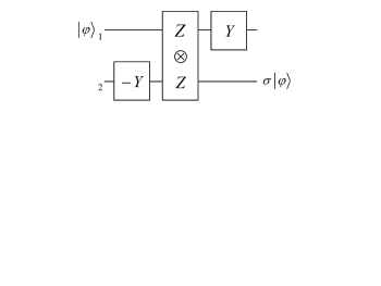
Figure 1: The state transfer based on $Y$-measurements.

The simulation step of $J(\theta)$ in [8] is based on the state transfer, which is a simplified version of quantum teleportation and uses $X$- and $Z\otimes Z$-measurements. For example, it implies a simulation step of $J(0)=H$ using $Z$-, $X$-, and $Z\otimes X$-measurements. To simplify this, our idea is to use the state transfer based on $Y$-measurements depicted in Fig. 1, which transfers the input state $|\varphi\rangle$ from qubit 1 to qubit 2 (up to Pauli operations). As in [8], this implies a simulation step of a unitary operation using projective measurements depending on the operation. For example, we can obtain a simulation step of $H$ by replacing $-Y$ and $Z\otimes Z$ with $H(-Y)H^{\dagger}=Y$ and $Z\otimes(HZH^{\dagger})=Z\otimes X$, respectively. The simulation step is simpler than the previous one since it uses only $Y$- and $Z\otimes X$-measurements.

On the basis of the idea, we show the following theorem:

Theorem 1

The set of observables

$${\cal S}_{1}=\{Z\otimes X,(\cos\theta)X+(\sin\theta)Y\ {\rm all}\ \theta\in[0,2\pi)\}$$

with one ancillary qubit is universal for quantum computation.

Proof. The set of gates

$$\{(P^{-1}\otimes HP^{-1})\Lambda Z(I\otimes H),J(\theta)\ {\rm all}\ \theta\in[0,2\pi)\}$$

is universal for quantum computation, where $P=Z(\pi/2)$ (and thus $P^{-1}=\sigma_{z}P$). This is because $J(\theta)$ generates any one-qubit gate and $\{\Lambda Z,J(\theta)\ {\rm all}\ \theta\in[0,2\pi)\}$ is universal for quantum computation [8, 14]. Thus, to show the theorem, it suffices to simulate any gate in the above set by projective measurements described by the observables in ${\cal S}_{1}$.

To give the simulation step of $J(\theta)$, we consider the procedure depicted in Fig. 2, which is obtained by replacing $-Y$, $Z\otimes Z$, and $Y$ in Fig. 1 with $H(-Y)H^{\dagger}=Y$, $(Z(\theta)^{\dagger}ZZ(\theta))\otimes(HZH^{\dagger})=Z\otimes X$, and $Z(\theta)^{\dagger}YZ(\theta)=\cos(\pi/2-\theta)X+\sin(\pi/2-\theta)Y$, respectively. Let $|\varphi\rangle=\alpha|0\rangle+\beta|1\rangle$ and $s_{1},s_{2},s_{3}\in\{1,-1\}$ be the classical outcomes of the measurements $Y^{(2)}$, $Z^{(1)}\otimes X^{(2)}$, and $(\cos(\pi/2-\theta)X+\sin(\pi/2-\theta)Y)^{(1)}$, respectively. The first measurement transforms the input state into

$$(I\otimes\sigma^{\frac{1-s_{1}}{2}}_{z})(\alpha|0\rangle+\beta|1\rangle)|+_{\frac{\pi}{2}}\rangle.$$

The second measurement transforms the state into

$$(\sigma^{\frac{1-s_{1}s_{2}}{2}}_{z}\otimes\sigma^{\frac{1-s_{2}}{2}}_{z})(\alpha|0\rangle|+\rangle-i\beta|1\rangle|-\rangle).$$

The third measurement transforms it into

$$(\sigma^{\frac{1-s_{3}}{2}}_{z}\otimes\sigma^{\frac{1-s_{2}}{2}}_{z}\sigma^{\frac{1+s_{1}s_{2}s_{3}}{2}}_{x})|+_{\frac{\pi}{2}-\theta}\rangle(\alpha|+\rangle+e^{i\theta}\beta|-\rangle),$$

which is the desired output state since $J(\theta)|\varphi\rangle=\alpha|+\rangle+e^{i\theta}\beta|-\rangle$. Thus, the procedure depicted in Fig. 2 is a simulation step of $J(\theta)$, where $\sigma=I,\ \sigma_{x},\ \sigma_{z},$ or $\sigma_{z}\sigma_{x}$ $(=\sigma_{y}$ up to a global phase). It can be shown that each $\sigma$ occurs with the same probability, 1/4.

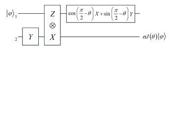
Figure 2: The simulation step of $J(\theta)$.

To give the simulation step of $(P^{-1}\otimes HP^{-1})\Lambda Z(I\otimes H)$, we consider the procedure depicted in Fig. 3. Let $|\varphi\rangle=\alpha|00\rangle+\beta|01\rangle+\gamma|10\rangle+\delta|11\rangle$ and $s_{1},s_{2},s_{3},s_{4}\in\{1,-1\}$ be the classical outcomes of the measurements $Y^{(3)}$ (the left one), $Z^{(1)}\otimes X^{(3)}$, $Z^{(3)}\otimes X^{(2)}$, and $Y^{(3)}$ (the right one), respectively. The first measurement transforms the input state into

$$(I\otimes I\otimes\sigma^{\frac{1-s_{1}}{2}}_{z})(\alpha|00\rangle+\beta|01\rangle+\gamma|10\rangle+\delta|11\rangle)|+_{\frac{\pi}{2}}\rangle.$$

The second measurement transforms the state into

$$(\sigma^{\frac{1-s_{1}s_{2}}{2}}_{z}\otimes I\otimes\sigma^{\frac{1-s_{2}}{2}}_{z})(\alpha|0\rangle|0\rangle|+\rangle+\beta|0\rangle|1\rangle|+\rangle-i\gamma|1\rangle|0\rangle|-\rangle-i\delta|1\rangle|1\rangle|-\rangle).$$

The third measurement transforms the state into

$$(\sigma^{\frac{1-s_{1}s_{2}s_{3}}{2}}_{z}\otimes\sigma^{\frac{1-s_{2}}{2}}_{x}\otimes\sigma^{\frac{1-s_{3}}{2}}_{x}) (\alpha|0\rangle\frac{|+\rangle|0\rangle+|-\rangle|1\rangle}{\sqrt{2}}+\beta|0\rangle\frac{|+\rangle|0\rangle-|-\rangle|1\rangle}{\sqrt{2}}$$

$$-i\gamma|1\rangle\frac{|+\rangle|0\rangle-|-\rangle|1\rangle}{\sqrt{2}}-i\delta|1\rangle\frac{|+\rangle|0\rangle+|-\rangle|1\rangle}{\sqrt{2}}).$$

The fourth measurement transforms it into

$$(\sigma^{\frac{1-s_{1}s_{2}s_{3}}{2}}_{z}\otimes\sigma^{\frac{1-s_{2}s_{3}s_{4}}{2}}_{x}\otimes\sigma^{\frac{1-s_{4}}{2}}_{z}) (\alpha|0\rangle\frac{|+\rangle-i|-\rangle}{\sqrt{2}}+\beta|0\rangle\frac{|+\rangle+i|-\rangle}{\sqrt{2}}$$

$$-i\gamma|1\rangle\frac{|+\rangle+i|-\rangle}{\sqrt{2}}-i\delta|1\rangle\frac{|+\rangle-i|-\rangle}{\sqrt{2}})|+_{\frac{\pi}{2}}\rangle,$$

which is the desired output state since

$$(P^{-1}\otimes HP^{-1})\Lambda Z(I\otimes H)|\varphi\rangle = \alpha|0\rangle\frac{|+\rangle-i|-\rangle}{\sqrt{2}}+\beta|0\rangle\frac{|+\rangle+i|-\rangle}{\sqrt{2}}$$

$$-i\gamma|1\rangle\frac{|+\rangle+i|-\rangle}{\sqrt{2}}-i\delta|1\rangle\frac{|+\rangle-i|-\rangle}{\sqrt{2}}.$$

Thus, the procedure depicted in Fig. 3 is a simulation step of $(P^{-1}\otimes HP^{-1})\Lambda Z(I\otimes H)$, where $\sigma=I\otimes I,\ I\otimes\sigma_{x},\ \sigma_{z}\otimes I,$ or $\sigma_{z}\otimes\sigma_{x}$. It can be shown that each $\sigma$ occurs with the same probability, 1/4.

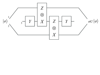
Figure 3: The simulation step of $U=(P^{-1}\otimes HP^{-1})\Lambda Z(I\otimes H)$.

To implement $\sigma_{x}$, we consider the procedure depicted in Fig. 4. Let $|\varphi\rangle=\alpha|0\rangle+\beta|1\rangle$ and $s_{1},s_{2},s_{3}\in\{1,-1\}$ be the classical outcomes of the measurements $Y^{(2)}$ (the left one), $X^{(1)}\otimes Z^{(2)}$, and $Y^{(2)}$ (the right one), respectively. The first measurement transforms the input state into

$$(I\otimes\sigma^{\frac{1-s_{1}}{2}}_{z})(\alpha|0\rangle+\beta|1\rangle)|+_{\frac{\pi}{2}}\rangle.$$

The second measurement transforms the state into

$$(I\otimes\sigma^{\frac{1-s_{1}}{2}}_{z}\sigma^{\frac{1-s_{2}}{2}}_{y})\frac{1}{\sqrt{2}}((\alpha|0\rangle+\beta|1\rangle)|+_{\frac{\pi}{2}}\rangle+(\alpha|1\rangle+\beta|0\rangle)|-_{\frac{\pi}{2}}\rangle).$$

The third measurement transforms the state into

$$(\sigma^{\frac{1-s_{1}s_{3}}{2}}_{x}\otimes\sigma^{\frac{1-s_{3}}{2}}_{z})(\alpha|0\rangle+\beta|1\rangle)|+_{\frac{\pi}{2}}\rangle.$$

It can be shown that $\sigma_{x}$ is implemented with the probability 1/2.

To implement $\sigma_{z}$, we consider the procedure depicted in Fig. 5. Let $|\varphi\rangle=\alpha|0\rangle+\beta|1\rangle$ and $s_{1},s_{2},s_{3}\in\{1,-1\}$ be the classical outcomes of the measurements $Y^{(2)}$ (the left one), $Z^{(1)}\otimes X^{(2)}$, and $Y^{(2)}$ (the right one), respectively. The first measurement transforms the input state into

$$(I\otimes\sigma^{\frac{1-s_{1}}{2}}_{z})(\alpha|0\rangle+\beta|1\rangle)|+_{\frac{\pi}{2}}\rangle.$$

The second measurement transforms the state into

$$(\sigma^{\frac{1-s_{1}s_{2}}{2}}_{z}\otimes\sigma^{\frac{1-s_{2}}{2}}_{z})(\alpha|0\rangle|+\rangle-i\beta|1\rangle|-\rangle).$$

The third measurement transforms the state into

$$(\sigma^{\frac{1-s_{1}s_{3}}{2}}_{z}\otimes\sigma^{\frac{1-s_{3}}{2}}_{z})(\alpha|0\rangle+\beta|1\rangle)|+_{\frac{\pi}{2}}\rangle.$$

It can be shown that $\sigma_{z}$ is implemented with the probability 1/2.

In the correction step, we repeat the procedures until the desired gate $(\sigma_{x}$ or $\sigma_{z})$ is implemented (as in [9]). The gate $\sigma_{y}$ is implemented by combining the procedures. Thus, any gate in the set described at the beginning of the proof can be simulated by projective measurements described by the observables in ${\cal S}_{1}$. $\Box$

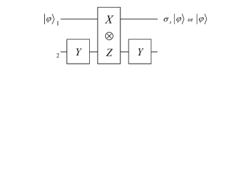
Figure 4: The implementation of $\sigma_{x}$ in the correction step.

Figure 5: The implementation of $\sigma_{z}$ in the correction step.

The proof of Theorem 1 immediately implies Perdrix’s result [9]:

Theorem 2

The set of observables

$${\cal S}_{2}=\{Z\otimes X,Y,(X+Y)/\sqrt{2}\}$$

with one ancillary qubit is approximately universal for quantum computation.

Proof. The set of gates $\{H,J(\pi/4),(P^{-1}\otimes HP^{-1})\Lambda Z(I\otimes H)\}$ is approximately universal for quantum computation. This is because $\{H,Z(\pi/4),\Lambda Z\}$ is approximately universal for quantum computation [4, 13], $H^{2}=I$, and $(HJ(\pi/4))^{2}=P$. On the basis of the set of gates, it is easy to show the theorem since the simulation steps of the gates and the correction steps in the proof of Theorem 1 use projective measurements described by the observables only in ${\cal S}_{2}$. $\Box$

We can also immediately imply other approximately universal sets of observables using other approximately universal sets of gates [15].

4 Efficient Graph State Preparation

Let $G=(V,E)$ be a graph with a set of vertices $V=\{1,\ldots,n\}$ and a set of edges $E\subseteq V\times V$. The graph state $|G\rangle$ that corresponds to the graph $G$ is the quantum state obtained by the following procedure, where we assume that we have the initial state $|0\rangle_{1}\cdots|0\rangle_{n}$ and call the $k$-th qubit the qubit corresponding to the vertex $k$:

1. Apply $H$ to the qubit corresponding to the vertex $k$ for any $k\in V$.

2. Apply $\Lambda Z$ to the pair of qubits corresponding to the vertices $k_{1}$ and $k_{2}$ for any $(k_{1},k_{2})\in E$.

We call this procedure the standard procedure. For example, the graph state $|G\rangle$ corresponding to the graph $G$ depicted in Fig. 6 is obtained by

$$\Lambda Z_{14}\Lambda Z_{23}\Lambda Z_{24}\Lambda Z_{34}H_{1}H_{2}H_{3}H_{4}|0\rangle_{1}|0\rangle_{2}|0\rangle_{3}|0\rangle_{4}.$$

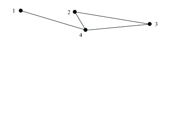
Figure 6: The graph $G$ with $V=\{1,2,3,4\}$ and $E=\{(1,4),(2,3),(2,4),(3,4)\}$.

We consider a quantum circuit for preparing graph states, where the circuit consists only of projective measurements. As in the standard quantum circuit model, the complexity measures of a quantum circuit are the number of qubits in it and its size and depth [16]. The size is the number of projective measurements and the depth is the number of layers in the circuit, where a layer consists of projective measurements that can be performed simultaneously. A quantum circuit can use ancillary qubits, which start in state $|0\rangle$.

We show that the set of observables ${\cal S}_{3}=\{Z\otimes X,Y\}$ with one ancillary qubit is sufficient for preparing graph states efficiently. From the proof of Theorem 1, we can simulate $H$ and $(P^{-1}\otimes HP^{-1})\Lambda Z(I\otimes H)$ using projective measurements described by the observables in ${\cal S}_{3}$. Thus, we can simulate $(P^{-1}\otimes P^{-1})\Lambda Z$. However, since ${\cal S}_{3}$ has only $Z\otimes X$ and $Y$, it is difficult to simulate $P$ and thus $\Lambda Z$. This means that it is difficult to use the standard procedure directly.

Our circuit consists of three steps. In Step 2, we use $(P^{-1}\otimes P^{-1})\Lambda Z$ in place of $\Lambda Z$ in Step 2 of the standard procedure. Since $P^{-1}$ and $\Lambda Z$ commute, this step is equivalent to Step 2 of the standard procedure up to local unitary gates generated by $P^{-1}$. We need to remove the side effects, that is, the local unitary gates, to obtain an exact graph state. If the degree of the vertex $k$ (that is, the number of edges incident to $k$) is even, $P^{-1}$ is applied to the qubit corresponding to the vertex $k$ even times and thus the local unitary gate is $(P^{-1})^{2}=\sigma_{z}$ or $(P^{-1})^{4}=I$. Similarly, if the degree is odd, the local unitary gate is $P^{-1}$ or $(P^{-1})^{3}=\sigma_{z}P^{-1}$.

Our idea of removing the side effects is that, in Step 1 of our circuit, we apply $H$ (or $\sigma_{z}H$) to the qubit corresponding to a vertex if the degree of the vertex is even and we perform a $Y$-measurement on the qubit to prepare $|-_{\frac{\pi}{2}}\rangle=P^{-1}H|0\rangle$ (or $|+_{\frac{\pi}{2}}\rangle=\sigma_{z}P^{-1}H|0\rangle$) if the degree is odd. Combining Step 1 with Step 2 transforms the side effects in Step 2 to only $\sigma_{z}$ or $I$. In Step 3, $\sigma_{z}$ is removed if needed. For example, our circuit for preparing the graph state $|G\rangle$ corresponding to the graph $G$ depicted in Fig. 6 is based on the circuit (in the standard quantum circuit model) depicted in Fig. 7. An ancillary qubit is reused to simulate $(P^{-1}\otimes P^{-1})\Lambda Z$ and $\sigma_{z}$.

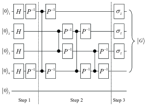
Figure 7: The quantum circuit for preparing $|G\rangle$ corresponding to the graph $G$ depicted in Fig. 6. The gate represented by two solid circles connected by a line is $\Lambda Z$. An ancillary qubit is reused to simulate $(P^{-1}\otimes P^{-1})\Lambda Z$ and $\sigma_{z}$.

On the basis of the idea, we show the following theorem, where we assume that we have a classical description of a given graph and can thus use the degree of a vertex to construct a quantum circuit:

Theorem 3

For any graph $G=(V,E)$, the graph state $|G\rangle$ can be prepared by a quantum circuit consisting of one-qubit and two-qubit projective measurements described by the observables in ${\cal S}_{3}=\{Z\otimes X,Y\}$ with size and depth $O(n+m)$ and one ancillary qubit, where $n=|V|$ and $m=|E|$.

Proof. Let $\deg(k)$ be the degree of the vertex $k$. We assume that we have the initial state $|0\rangle_{1}\cdots|0\rangle_{n+1}$ and the $(n+1)$-th qubit is an ancillary qubit. Our circuit is constructed by using the following procedure:

1. For $k=1,\ldots,n$:

   • If $\deg(k)\equiv 0\ \rm mod\,2$, apply the simulation step of $H$ where the qubit corresponding to the vertex $k$ is used as an ancillary qubit and the qubit corresponding to the vertex $k+1$ (in state $|0\rangle$) is used as an input qubit. Let $t_{k}$ be the classical outcome of the $Z\otimes X$-measurement in the simulation step. The resulting state of the qubit corresponding to the vertex $k$ is $H|0\rangle$ if $t_{k}=1$ and $\sigma_{z}H|0\rangle$ otherwise.

   • If $\deg(k)\equiv 1\ \rm mod\,2$, perform a $Y$-measurement on the qubit corresponding to the vertex $k$. Let $u_{k}$ be the classical outcome of the measurement. The resulting state of the qubit is $|+_{\frac{\pi}{2}}\rangle=\sigma_{z}P^{-1}H|0\rangle$ if $u_{k}=1$ and $|-_{\frac{\pi}{2}}\rangle=P^{-1}H|0\rangle$ otherwise.

2. Apply $(P^{-1}\otimes P^{-1})\Lambda Z$ as in Step 2 of the standard procedure, where we reuse an ancillary qubit.

3. For $k=1,\ldots,n$:

   If one of the following conditions holds, apply $\sigma_{z}$ to the qubit corresponding to the vertex $k$, where we reuse an ancillary qubit:

   • $\deg(k)\equiv 0\ \rm mod\,4$ and $t_{k}=-1$.

   • $\deg(k)\equiv 1\ \rm mod\,4$ and $u_{k}=-1$.

   • $\deg(k)\equiv 2\ \rm mod\,4$ and $t_{k}=1$.

   • $\deg(k)\equiv 3\ \rm mod\,4$ and $u_{k}=1$.

From the proof of Theorem 1, the above procedure can be done by using projective measurements described by the observables in ${\cal S}_{3}$. It is easy to show that the circuit works correctly and that the size and depth are $O(n+m)$ and the circuit uses only one ancillary qubit. $\Box$

The depth of our circuit is larger than Høyer et al.’s one. Since the graph states corresponding to connected graphs seem to be particularly useful in quantum information processing, we are interested in such graphs. For a connected graph, $m=\Omega(n)$ and thus the depth of our circuit is $O(m)$ in this case, which is asymptotically the same as Høyer et al.’s one.

5 Conclusions and Future Work

We showed that the set of observables $\{Z\otimes X,(\cos\theta)X+(\sin\theta)Y\ {\rm all}\ \theta\in[0,2\pi)\}$ with one ancillary qubit is universal. This improves Jorrand and Perdrix’s result and the proof immediately implies the best known result for the approximate universality by Perdrix. The proof also implies that the set of observables $\{Z\otimes X,Y\}$ with one ancillary qubit is sufficient for preparing graph states efficiently. It would be interesting to investigate whether our result can be improved or not. For example, is there a set of one one-qubit observable and one two-qubit observable that is approximately universal for quantum computation using one ancillary qubit?

References

- [1] R. Raussendorf and H. J. Briegel, A one-way quantum computer, Phys. Rev. Lett. 86 (2001) 5188–5191.
- [2] D. Gottesman and I. L. Chuang, Quantum teleportation as a universal computational primitive, Nature 402 (1999) 390–393.
- [3] M. A. Nielsen, Quantum computation by measurement and quantum memory, Phys. Lett. A 308 (2003) 96–100.
- [4] M. A. Nielsen and I. L. Chuang, Quantum Information and Quantum Computation (Cambridge University Press, 2000).
- [5] S. Perdrix, State transfer instead of teleportation in measurement-based quantum computation, International Journal of Quantum Information, Vol. 3 No. 1 (2005) 219–223.
- [6] A. M. Childs, D. W. Leung, and M. A. Nielsen, Unified derivation of measurement-based schemes for quantum computation, Phys. Rev. A 71 (2005) 032318.
- [7] D. W. Leung, Quantum computation by measurements, International Journal of Quantum Information, Vol. 2 No. 1 (2004) 33–43.
- [8] P. Jorrand and S. Perdrix, Unifying quantum computation with projective measurements only and one-way quantum computation, Proc. SPIE Quantum Informatics 2004, Vol. 5833 (2005) 44–51.
- [9] S. Perdrix, Towards minimal resources of measurement-based quantum computation, New Journal of Physics 9 (2007) 206.
- [10] M. Hein, W. Dür, J. Eisert, R. Raussendorf, M. Van den Nest, and H. J. Briegel, Entanglement in graph states and its applications, Proc. International School of Physics “Enrico Fermi” on “Quantum Computers, Algorithms and Chaos”, (2005).
- [11] P. Høyer, M. Mhalla, and S. Perdrix, Resources required for preparing graph states, Proc. International Symposium on Algorithms and Computation 2006, LNCS Vol. 4288 (2006) 638–649.
- [12] A. Barenco, C. H. Bennett, R. Cleve, D. P. DiVincenzo, N. Margolus, P. Shor, T. Sleator, J. A. Smolin, and H. Weinfurter, Elementary gates for quantum computation, Phys. Rev. A, Vol. 52 No. 5 (1995) 3457–3467.
- [13] P. O. Boykin, T. Mor, M. Pulver, V. Roychowdhury, and F. Vatan, A new universal and fault-tolerant quantum basis, Information Processing Letters, Vol. 75 No. 3 (2000) 101–107.
- [14] V. Danos, E. Kashefi, and P. Panangaden, Parsimonious and robust realizations of unitary maps in the one-way model, Phys. Rev. A 72 (2005) 064301.
- [15] Y. Shi, Both Toffoli and Controlled-NOT need little help to do universal quantum computing, Quantum Information and Computation, Vol. 3 No. 1 (2003) 84–92.
- [16] Y. Takahashi, Quantum arithmetic circuits: a survey, IEICE Trans. Fundamentals, Vol. E92-A No. 5 (2009) 1276–1283.