Rigorous formulation of oblique incidence scattering from dispersive media

Abstract

We formulate a finite-difference time-domain (FDTD) approach to simulate electromagnetic wave scattering from scatterers embedded in layered dielectric or dispersive media. At the heart of our approach is a derivation of an equivalent one-dimensional wave propagation equation for dispersive media characterized by a linear sum of Debye-, Drude- and Lorentz-type poles. The derivation is followed by a detailed discussion of the simulation setup and numerical issues. The developed methodology is tested by comparison with analytical reflection and transmission coefficients for scattering from a slab, illustrating good convergence behavior. The case of scattering from a sub-wavelength slit in a dispersive thin film is explored to demonstrate the applicability of our formulation to time- and incident angle-dependent analysis of surface waves generated by an obliquely incident plane wave.

I INTRODUCTION

The study of obliquely incident plane wave upon planar interfaces is of fundemantal interest to electromagnetic (EM) wave propagation. It underlies Snell’s law of refraction and leads to important concepts such as total reflection and Brewster’s angle.Jackson ; Wolf One can easily relate to the concept of an obliquely incident plane wave by the daily experience of looking into a mirror. In practice, oblique incidence is vastly applied in EM related applications such as fiber optics,Hecht underground object detection,Jol and RF-human body interaction.Vorst

In the growing field of nanoplasmonics,Barnes ; Ozbay oblique incidence finds applications particularly in exciting surface plasmon polaritons (SPPs), exemplified by the common experimental setup in which subwavelength defects or attenuated total reflection are utilized to couple the obliquely incident plane wave into propagating SPPs.Lopez ; Coe By taking advantage of the incident angle degree of freedom, several experiments have demonstrated SPP near-field manipulation,Yin ; Liu ; Doui which has been proposed as a direct approach to measuring SPP generation efficiency.Wang Most recently, it has been shown that SPP’s can be directly generated on a planar metal surface by interfering incoming light beams with different incident angles in a four-wave mixing scheme.Renger

The effects of light incident at oblique angle on sub-wavelength defects in metallic layered media have been studied by frequency-domain calculations based on either coupled wave analysis or a semi-analytical model. These references have explored the obliquely incident light transmission through a single defect,Vidal1 ; Vidal2 ; Gordon and the SPP generation efficiency.Lalanne ; Kim Our work is largely motivated by recent experimental study of SPP dynamics excited or controlled by a femto-second (fs) laser pulse obliquely incident on a SPP propagating interface.MacDonald ; footnote0 To describe such experiments, a time-domain method is desirable because of the ultrafast nature of the exciting or controlling laser pulse. The major challenge in developing such a method, is to accurately treat the oblique incidence as well as the material dispersiveness. This poses a special challenge for mesh-based propagation method (such as the finite-difference time domain method) because even in the absence of the inhomogeneous media the wave front not aligned with the Cartesian mesh is required to be uniform and to have arbitrary incident angle and time profile.

In this paper, we develop a numerical method to rigorously treat obliquely incident plane wave scattering at embedded scatterers in layered dielectric and dispersive media. To the best of our knowledge, such a method was not published as yet.ftnt1 Targetted mainly at time-domain studies of EM wave phenomena that involve SPP excitation and propagation in metallic films, the developed method is formulated within the framework of the finite-difference time-domain (FDTD) method. This method has enjoyed a wide range of applications in the field of nanoplasmonics,Taflove ; Teixeira and its time-domain nature makes it particularly well suited to ultrafast phenomena. Our treatment of the oblique plane wave is an extension of the total field / scatter field (TF/SF) technique to describe media characterized by the combination of Debye-, Drude- and Lorentz-type poles.Ung ; Lee The TF/SF technique has been applied successfully in the FDTD study of free-standing scatterers, layered dielectrics and dispersive media describable by a single Debye pole.Taflove ; Winton ; Capoglu ; Jiang It is based on the linearity of Maxwell’s equations and decomposes the total field into an incident and a scattered field components,Taflove

$$\psi^{\rm tot}=\psi^{\rm inc}+\psi^{\rm sca}.$$ (1)

By setting up an artificial boundary between the TF and SF regions in the FDTD simulations, a plane wave of arbitrary time profile and incident angle can be achieved by matching the known incident field at the TF and SF boundary. In presenting our method, we will focus on the derivation of an equivalent one-dimensional (1D) wave equations for the TF/SF boundary condition, suitable for various types of material dispersiveness, and explain in detail the numerical considerations involved. This will be followed by extensive numerical tests of the convergence properties of the method. For clarity, several important concepts from the previous literature are reemphasized.

This paper is organized as follows: In Section II, we derive the equivalent 1D wave equations, show the numerical flow chart for matching the TF/SF boundary condition, and discuss several practical simulation details, including stability, interface treatment, and leakage. Section III tests our approach by comparison of numerical with analytical results for model problems. Finally, concluding remarks are provided in Section IV.

II THEORY AND NUMERICAL METHOD

In the following, we provide the equations and numerical method for solving the transverse magnetic (TM) mode in two dimensions (magnetic field perpendicular to the two-dimensional plane). Special emphasis is placed on the TM mode because of its relevance to SPP excitation.Raether The numerical approach for solving the transverse electric (TE) mode equations is similar to that for the TM mode, and the corresponding equations are given in Appendix A. The media considered are vacuum, linear dielectric media (characterized by a dielectric constant), and linear dispersive media (characterized by a finite sum of Debye, Lorentz, and Drude types of poles).

II.1 TM mode wave propagation: two-dimensional and equivalent one-dimensional equations

Our starting point is Maxwell’s equations in the frequency domain for the TM mode,

$$\frac{\partial E_{y}}{\partial x}-\frac{\partial E_{x}}{\partial y}=i\omega\mu_{0}H_{z},$$ (2)

$$\frac{\partial H_{z}}{\partial y}=-i\omega\epsilon_{0}\epsilon(\omega)E_{x},$$ (3)

$$\frac{\partial H_{z}}{\partial x}=i\omega\epsilon_{0}\epsilon(\omega)E_{y},$$ (4)

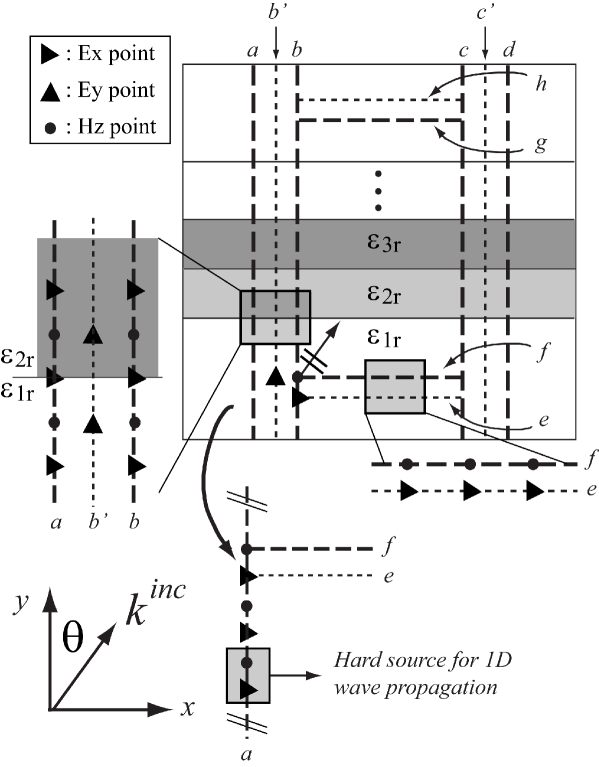
Figure 1: Simulation geometry: the layered media are distinguished by different shades and denoted by $\epsilon_{1r}$, $\epsilon_{2r}$, etc. Thick, dashed (thin, dotted) lines denote the boundaries to which the $H-$ ($E-$) field is assigned. The left, lower left, and lower right panels show the specific field point assignment at the interface, along line $a$, and at the horizontal boundaries, respectively. The $x$-coordinates of lines $a$, $b^{\prime}$, $b$, $c$, $c^{\prime}$, $d$ are $i_{1}-1/2$, $i_{1}$, $i_{1}+1/2$, $i_{2}-1/2$, $i_{2}$, and $i_{2}+1/2$, respectively. The $y$-coordinates of lines $e$, $f$, $g$, and $h$ are $j_{1}$, $j_{1}+1/2$, $j_{2}-1/2$, and $j_{2}$, respectively.

where the coordinate system is defined in Fig. 1, $\epsilon_{0}$ is the free space permitivity, $\mu_{0}$ is the free space permeability, and $\epsilon(\omega)$ is the dielectric function for a dispersive media, which reduces to a constant for vacuum and dielectric media.

In the case studies below, we assume a dispersive medium with a single (non-zero) Drude pole $\epsilon_{m}=\epsilon(\infty)-\omega_{D}^{2}/(\omega^{2}+i\Gamma_{D}\omega)$ and provide two separate sets of equations for solving Eqs. (2-4). The first set of equations is based on the auxiliary differential equation (ADE) approach with polarization currents to account for the dispersiveness. In this case, we further assume that media other than vacuum are not extended into the absorbing boundary, which allows us to use Berenger’s PML absorbing boundary condition.Berenger The second set of equations is formulated within the general context of the Uniaxial Perfectly Matched Layers (UPML) absorbing boundary conditions,Gedney and involves a different approach to treat the dispersiveness. In this case, we can effectively absorb the outgoing waves exiting the simulation domain in the dielectric and dispersive media. Separate tests have been done to ensure that the two approaches provide the same solution.footnote1 In the following, we assume that the 2D electric and magnetic fields propagate on the Yee mesh with the dependence $u|^{n}_{i,j}=u(i\Delta x,j\Delta y,n\Delta t)$. $\Delta x=\Delta y$ is the size of a unit cell, and $\Delta t$ is unit time step. Details on the FDTD equations in both ADE and UPML approaches are given in Appendix B.

If we now consider TM mode wave propagation with obliquely incident plane wave on layered media with translational invariance, the 2D equations of motion can be reduced to an equivalent 1D wave propagation problem along the direction perpendicular to the interfaces between the media.Winton ; Capoglu We proceed to derive the equivalent 1D wave equation for the TM mode, which will serve as a means of introducing incident fields along the TF/SF boundary. The corresponding derivation for the TE mode is provided in Appendix A.

Substituting Eq. (4) into Eq. (2) yields,

$$\frac{\partial E_{x}}{\partial y}=-i\omega\mu_{0}H_{z}+\frac{1}{i\omega\epsilon_{0}\epsilon(\omega)}\frac{\partial^{2}H_{z}}{\partial x^{2}}.$$ (5)

Because of the translational invariance and phase matching across the interfaces between different layers, ${\partial^{2}H_{z}}/{\partial x^{2}}=-k_{x}^{2}H_{z}$, with $k_{x}$ being a wavevector that is identical for waves in different layers.footnote2 If we further assume that an oblique plane wave is incident from a dielectric medium with relative permitivity $\epsilon_{1r}$, then $k_{x}=\omega\sqrt{\mu_{0}\epsilon_{0}\epsilon_{1r}}\sin(\theta)$, which can be substituted into Eq. (5) to give,

$$\frac{\partial E_{x}}{\partial y}=-i\omega\mu_{0}\left[\frac{\epsilon(\omega)-\epsilon_{1r}\sin^{2}(\theta)}{\epsilon(\omega)}\right]H_{z}.$$ (6)

Equations (3) and (6) constitute a system of equations for 1D TM wave propagation across the interfaces between the media. To translate those equations into FDTD equations, Jiang et al. introduced a convenient method to overcome the difficulty of time-domain convolution between the term in the square bracket and $H_{z}$ in Eq. (6). In this method,Jiang Eq. (6) is first split into a pair of equations as,

$$\frac{\partial E_{x}}{\partial y}=-i\omega\mu_{0}H_{z}^{\prime},$$ (7)

$$H_{z}^{\prime}=\frac{\epsilon(\omega)-\epsilon_{1r}\sin^{2}(\theta)}{\epsilon(\omega)}H_{z}.$$ (8)

Equations (3), (7) and (8) then lead to the following set of FDTD equations,

$$E_{x1D}|^{n+1}_{j} = a_{x1}E_{x1D}|^{n}_{j}+a_{x2}(H_{z1D}|^{n+1/2}_{j+1/2}-H_{z1D}|^{n+1/2}_{j-1/2})$$ (9)

$$+a_{x3}J_{x1D}|^{n+1/2}_{j},$$

$$J_{x1D}|^{n+3/2}_{j} = a_{x4}J_{x1D}|^{n+1/2}_{j}+a_{x5}E_{x1D}|^{n+1}_{j},$$ (10)

$$H^{\prime}_{z1D}|^{n+3/2}_{j+1/2} = b_{y1}H^{\prime}_{z1D}|^{n+1/2}_{j+1/2}+b_{y2}(E_{x1D}|^{n+1}_{j+1}-E_{x1D}|^{n+1}_{j}),$$ (11)

$$H_{z1D}|^{n+3/2}_{j+1/2} = b_{y3}H_{z1D}|^{n+1/2}_{j+1/2}+b_{y4}H_{z1D}|^{n-1/2}_{j+1/2}$$ (12)

$$+b_{y5}H^{\prime}_{z1D}|^{n+3/2}_{j+1/2}+b_{y6}H^{\prime}_{z1D}|^{n+1/2}_{j+1/2}$$

$$+b_{y7}H^{\prime}_{z1D}|^{n-1/2}_{j+1/2}.$$

In obtaining Eq. (12), we have multiplied both sides of Eq. (8) by $\epsilon(\omega)$ and Fourier transformed the result into the time domain. We have also made the assumption that a Drude model is used, $\epsilon_{m}=\epsilon(\infty)-\omega_{D}^{2}/(\omega^{2}+i\Gamma_{D}\omega)$. The updating coefficients in Eq. (12) are

$$\begin{cases}b_{y3}=b_{y4}=b_{y6}=b_{y7}=0\\ b_{y5}=\epsilon_{r}/\left[\epsilon_{r}-\epsilon_{1r}\sin^{2}(\theta)\right]\\ \end{cases}$$ (13)

in vacuum ($\epsilon_{r}=1$) and dielectric media (constant $\epsilon_{r}$), and

$$\begin{cases}b_{y3}=\frac{4\left[\epsilon(\infty)-\epsilon_{1r}\sin^{2}(\theta)\right]}{(2+\Gamma_{D}\Delta t)\left[\epsilon(\infty)-\epsilon_{1r}\sin^{2}(\theta)\right]+\omega_{D}^{2}\Delta t^{2}},\\ b_{y4}=-\frac{(2-\Gamma_{D}\Delta t)\left[\epsilon(\infty)-\epsilon_{1r}\sin^{2}(\theta)\right]+\omega_{D}^{2}\Delta t^{2}}{(2+\Gamma_{D}\Delta t)\left[\epsilon(\infty)-\epsilon_{1r}\sin^{2}(\theta)\right]+\omega_{D}^{2}\Delta t^{2}},\\ b_{y5}=\frac{(2+\Gamma_{D}\Delta t)\epsilon(\infty)+\omega_{D}^{2}\Delta t^{2}}{(2+\Gamma_{D}\Delta t)\left[\epsilon(\infty)-\epsilon_{1r}\sin^{2}(\theta)\right]+\omega_{D}^{2}\Delta t^{2}},\\ b_{y6}=\frac{-4\epsilon(\infty)}{(2+\Gamma_{D}\Delta t)\left[\epsilon(\infty)-\epsilon_{1r}\sin^{2}(\theta)\right]+\omega_{D}^{2}\Delta t^{2}},\\ b_{y7}=\frac{(2-\Gamma_{D}\Delta t)\epsilon(\infty)+\omega_{D}^{2}\Delta t^{2}}{(2+\Gamma_{D}\Delta t)\left[\epsilon(\infty)-\epsilon_{1r}\sin^{2}(\theta)\right]+\omega_{D}^{2}\Delta t^{2}}\\ \end{cases}$$ (14)

in Drude media. Here, we note the similarity between the updates of the $(H^{\prime},H)$ pair and the $(P,D)$ pair in the UPML formulation, which results from the fact that both pairs involves updating an auxiliary variable before the treatment of the material dispersiveness. In the case that $\epsilon(\omega)$ contains a linear sum of different types of poles (e.g., to accurately describe metals near inter-band transition energiesLee ), direct Fourier transform may not be as efficient because of higher-order derivatives with respect to time. For a systematic treatment of this situation, interested readers are referred to Appendix C. The updating coefficients in Eqs. (9) to (11) are identical to those in Eqs. (35), (36) and (40), which are given in Eqs. (42-46). We note that the updating coefficients corresponding to Berenger’s PML formulation can be used here provided that the two end media in the layers are vacuum. In the case of non-vacuum semi-infinite media at the two ends, 1D UPML can be used to effectively absorb the outgoing waves, for example, equations similar to Eqs. (47-49, 53, 54) can be used by setting $\kappa_{x}=1$ and $\sigma_{x}=0$ in Eqs. (59) and (61).

II.2 Simulation setup and flow chart

The main panel of Fig. 1 illustrates the geometry of the FDTD simulation region. The layered media are denoted by $\epsilon_{1r}$, $\epsilon_{2r}$, etc. and are stacked along the $y$ direction. The thick, dashed (thin, dotted) lines denote the TF/SF boundaries along which the incident $H$-field ($E$-field) is calculated. Incident field alignments on the boundaries are shown more explicitly in the zoom-in panels to the left and below the main panel. In this work, we assume that the oblique incidence field is introduced from the lower left corner (crossing point between lines $b$ and $f$ in the main panel of Fig. 1) with incident angle $\theta$ to the normal of the media interfaces ($y$ direction). We further assume that the two end media in the layers are vacuum. Consequently $\epsilon_{1r}=1$, so that field propagation along the horizontal boundaries $e$ through $h$ can be readily calculated by a delay of the free-space propagation time. In addition, the 1D field propagation along the vertical lines can be terminated by Berenger’s PML formulation. The perfectly matched layers absorbing boundaries are not shown in Fig. 1. They will be further illustrated and explained when we consider specific examples in Section III. The lower left panel in Fig. 1 shows the field alignment along line $a$ for the 1D wave propagation. The same setup applies to lines $b$, $c$ and $d$. Importantly, a 1D total field / scattered field approach is used here (the boundary points are highlighted in the shaded rectangle) because we must allow the wave from the multiple interface reflection to exit the 1D simulation and be absorbed at the bottom on the 1D simulation line.Capoglu

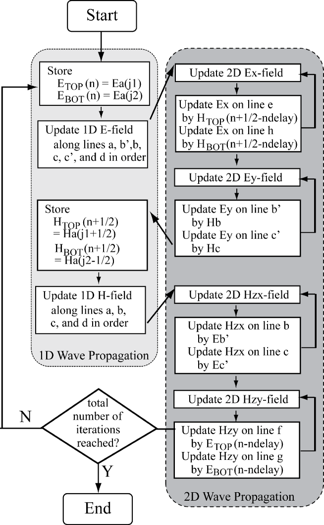
Figure 2: Simulation flow chart. Note that “TOP” (“BOT”) refers to a lower (higher) $y$ coordinate. For 1D field updates an Auxiliary Differential Equation (ADE) approach is used, while 2D field updates are performed by either the ADE approach or the equations consistent with the Uniaxial Perfectly Matched Layers (UPML) formulation.

Our simulation follows the flow chart shown in Fig. 2. The procedures belonging to 1D and 2D field updates are highlighted in the shaded rounded rectangles. In each iteration, the code updates the 1D $E$-field, 2D $E$-field, 1D $H$-field, and 2D $H$-field in a sequence. The order of 1D field storage and its matching to 2D simulation are important to ensure correct implementation of the 2D TF/SF scheme. Before updating the 1D field, the code needs to store at each time instant the 1D field values at the crossing points between line $a$ and lines $e$, $f$, $g$, and $h$.

The field matching at the TF/SF boundary is performed differently in accordance with the different updating schemes introduced in Section II.1. In the ADE approach, the TF/SF boundary matching equations on lines $e$, $f$, $b$ read,

$$E^{\rm sca}_{x}|^{n+1}_{i+1/2,j1} = E^{\rm sca}_{x}|^{n+1}_{i+1/2,j1}-a_{x2}H^{inc}_{zy}|^{n+1/2}_{i+1/2,j1+1/2},$$ (15)

$$H^{\rm tot}_{zy}|^{n+3/2}_{i+1/2,j1+1/2} = H^{\rm tot}_{zy}|^{n+3/2}_{i+1/2,j1+1/2}-b_{y2}E^{\rm sca}_{x}|^{n+1}_{i+1/2,j1},$$ (16)

$$H^{\rm tot}_{zx}|^{n+3/2}_{i1+1/2,j+1/2} = H^{\rm tot}_{zx}|^{n+3/2}_{i1+1/2,j+1/2}-b_{x2}E^{\rm sca}_{y}|^{n+1}_{i1,j+1/2}.$$ (17)

These updates are performed immediately after Eqs. (35), (40), and (39). For the $E_{y}$-field update on lines $b^{\prime}$ and $c^{\prime}$, because $J_{y}$ depends on the updated value of $E_{y}$ in Eq. (38), the $E_{y}$ boundary matching is performed in between Eqs. (37) and (38), for example, on line $b^{\prime}$,

$$E^{\rm sca}_{y}|^{n+1}_{i1,j+1/2}=E^{\rm sca}_{y}|^{n+1}_{i1,j+1/2}-a_{y2}H^{inc}_{zx}|^{n+1/2}_{i1+1/2,j+1/2}.\\$$ (18)

In the UPML formulation, the TF/SF boundary matching is carried out immediately after the $P$ and $B$ updates (before updating $D$ and $H$) in Eqs. (47-54), for example, the updates on lines $b$ and $b^{\prime}$ read

$$P^{\rm sca}_{y}|^{n+1}_{i1,j+1/2} = P^{\rm sca}_{y}|^{n+1}_{i1,j+1/2}-\alpha_{y1}H^{inc}_{z}|^{n+1/2}_{i1+1/2,j+1/2},$$ (19)

$$B^{\rm tot}_{z}|^{n+3/2}_{i1+1/2,j+1/2} = B^{\rm tot}_{z}|^{n+3/2}_{i1+1/2,j+1/2}-\beta_{2}E^{\rm sca}_{y}|^{n+1}_{i1,j+1/2}.$$ (20)

Because the above updates are performed between the updates of $P$ and $D$ or $B$ and $H$, they are indicated in the flow chart (Fig. 2) by the upward arrows on the right. We note that if the same type of PML absorbing boundary condition is used to terminate both the 1D and the 2D field propagation, one can allow them to have the same updating coefficients in the PML region and therefore remove the procedures of saving and matching the field components on lines $g$ and $h$ [$E_{\rm BOT}$ and $H_{\rm BOT}$].Jiang This particular setup is useful in the description of a very thick bottom layer (semi-infinite in the positive $y$ direction).

In the case of normal incidence, the code simplifies in two ways. First, in Eq. (8), $H=H^{\prime}$, and therefore Eq. (12) is removed from the 1D $H$-field update procedure. Second, it is not necessary to store and interpolate the field values $E_{\rm BOT}$, $E_{\rm TOP}$, $H_{\rm BOT}$, and $H_{\rm TOP}$, because field excitation is synchronized along lines $e$, $f$, $g$ and $h$, respectively.

The incident field values on lines $a$, $b$, $c$ and $d$ are calculated from Eqs. (9-12) using a 1D TF/SF scheme that allows fields reflected from the interfaces to exit the 1D simulation domain. Based on the geometry shown in the lower left panel in Fig. 1, we assume that the incoming $H$-field with time-dependence $f(t)$ excites the 1D field at point $(i1-1/2,j1-3/2)$. Paired with this excitation is an $E$-field of the form $g(t)=-\sqrt{\mu_{0}/\epsilon_{0}}f(t+\Delta x\cos(\theta)/2c)\cos(\theta)$, exciting the 1D field at point $(i1-1/2,j1-2)$. For example, on line $a$ in Fig. 1, the 1D TF/SF boundary matching equations read,

$$E^{\rm sca}_{a}|^{n+1}_{j1-2} = E^{\rm sca}_{a}|^{n+1}_{j1-2}-a_{x2}f|^{n+1/2},$$ (21)

$$H^{\rm\prime tot}_{a}|^{n+3/2}_{j1-3/2} = H^{\rm\prime tot}_{a}|^{n+3/2}_{j1-3/2}-b_{y2}g|^{n+1}.$$ (22)

The values of $f|^{n+1/2}$ and $g|^{n}$ are calculated from the known expressions of $f(t)$ and $g(t)$ using time-domain interpolation when necessary. These values are stored at each instant to generate the excitation fields for lines $b$, $c$, and $d$ by introducing a time delay $t_{delay}=N\Delta x\sin(\theta)/c$. The field values on the horizontal lines $e$, $f$, $g$ and $h$ are obtained in a similar fashion. One can also store the field values at each point on line $a$, and save the computation along lines $b$, $c$ and $d$ by introducing a proper time delay. This scheme reduces the computation time for the cost of larger memory requirement. Finally, the 2D TF/SF boundary values [$E^{\rm inc}_{y}$] along lines $b^{\prime}$ ($c^{\prime}$) are readily calculated from the $H$-field values on lines $a$ and $b$ ($c$ and $d$) using Eqs. (37) and (38). In addition, we note that the excitation and PML absorbing boundary conditions are enforced on $H^{\prime}$ in the 1D field updates.

Several practical issues should be considered. First, in vacuum, the projection of the phase velocity of the oblique incident field on the $y$-axis is $c/\cos(\theta)$. As the incident angle $\theta$ increases, the phase velocity can be very large and cause numerical instability if a fixed Courant criterium is enforced (e.g., $\Delta t=\Delta x/2c$). Based on this observation, we vary the Courant number $S=c\Delta t/\Delta x$ to ensure stability. When the incident angle is small, a small Courant number is used to ensure resolution of the time domain interpolation along the horizontal boundaries. In our simulation, the same Courant number is used for both 1D and 2D wave propagations, while an interpolation scheme to match different Courant numbers in 1D and 2D wave propagations is explained in Ref. Capoglu, . Second, as the dielectric function is discontinuous across the interface between layers of different media, we have used an average dielectric function for updating the fields at the interface.Zhao ; Mohammadi1 For example, in the left panel of Fig. 1, we use the dielectric function $\epsilon_{\rm eff}=(\epsilon_{1r}+\epsilon_{2r})/2$ for the $E_{x}$-field updates at the interface. In Section III, we will show that this scheme leads to faster convergence and/or higher accuracy as compared to the standard step-like change of $\epsilon$. Finally, we use a Gaussian ramping in the hard source time-response in Eqs. (21) and (22) to slowly ramp the field to continuous wave so as to avoid high-frequency component leakage out of the TF/SF domain. Specifically, $f(t)=\exp(-(t-\tau_{dealy})^{2}/\tau_{0}^{2})\sin(\omega t)$, $\tau_{delay}=30$ fs, $\tau_{0}=10$ fs, for the ramping phase $0<t<\tau_{delay}$.

II.3 Numerical tests

To test the accuracy of the TF/SF scheme, we compare our simulation results to analytical results by considering the oblique TM wave incident upon a slab sandwiched between two vacuum media. The analytical results for the reflection and transmission coefficients are given byWolf

$$r = \frac{r_{12}+r_{23}e^{2i\gamma}}{1+r_{12}r_{23}e^{2i\gamma}},$$ (23)

$$t = \frac{t_{12}t_{23}e^{i\gamma}}{1+r_{12}r_{23}e^{2i\gamma}}.$$ (24)

For TM wave,

$$r_{ij} = \frac{\cos(\theta_{i})/n_{i}-\cos(\theta_{j})/n_{j}}{\cos(\theta_{i})/n_{i}+\cos(\theta_{j})/n_{j}},$$ (25)

$$t_{ij} = \frac{2\cos(\theta_{i})/n_{i}}{\cos(\theta_{i})/n_{i}+\cos(\theta_{j})/n_{j}},$$ (26)

$$\sin(\theta_{i}) = \frac{n_{j}}{n_{i}}\sin(\theta_{j}),$$ (27)

$$\gamma = \frac{\omega}{c}n_{2}h\cos(\theta_{2}).$$ (28)

Here, $r_{ij}$ and $t_{ij}$ denote, respectively, the reflection and transmission coefficients at the interface between media $i$ and $j$, and $n_{i}=\sqrt{\epsilon_{i}(\omega)}$ denotes the refractive index of media $i$. We assume that medium $2$ is a slab of thickness $h$. The waves at the input side of the slab, where the incident and reflected waves propagate, and at the output side, where the transmitted wave propagates, can then be expressed as,

$$\psi^{\rm input} = \exp[i(k_{x}x+k_{y}y)]+r\exp[i(k_{x}x-k_{y}y)],$$ (29)

$$\psi^{\rm output} = t\exp[i(k_{x}x+k_{y}y)].$$ (30)

The above expressions indicate that the maximum field amplitude on the input and output sides are $1+|r|$ and $|t|$, respectively. These quantities can be obtained along a $y$-direction detection line in the TF/SF scheme for layered media without placing any scatterer inside the TF region. Using this scheme, we also test the leakage, defined as the ratio of the maximum field magnitude in the scattered field region to the maximum field magnitude in the total field region: ${\rm leakage}={\rm max}|\psi^{\rm sca}|^{n}_{i,j}|/{\rm max}|\psi^{\rm tot}|^{n}_{i,j}|$, where $\psi$ refers to $E_{x}$, or $E_{y}$, or $H_{z}$. In the ideal case, ${\rm leakage}=0$, whereas in practice, ${\rm leakage}<10^{-2}$ (or $-40$ dB) is desirable.Taflove Specific numerical examples of the tests are provided in Section III, where “leakage” refers to the largest leakage among $E_{x}$, or $E_{y}$, or $H_{z}$. In addition, we have tested the accuracy of the wave propagation in the layered media by inspecting the $x$ and $y$ projections of the wavelength [where, for instance, the $x$-projection is $2\pi/k_{x}$ and $k_{x}=k\sin(\theta)$]. In the case of a dispersive slab, we have also tested the skin depth (the distance where the field decays to $e^{-1}$ of its value at the surface, ca. 30 nm for the Drude model and parameters in our calculation), by considering a slab with thickness larger than $300$ nm. These tests all show an error within $5\%$ compared to analytical results.

III Numerical examples and discussions

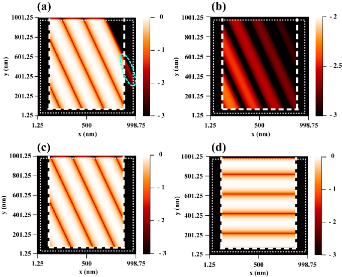
Figure 3: (color online) In panels (a–c), the incident plane wave enters the TF region from the lower left corner of the TF/SF boundary with incident angle $\theta=65^{\circ}$. (a) Magnetic ($H$) field snapshot at $3.00$ fs for a plane wave propagating in vacuum. The dashed oval indicates the leakage outside the TF/SF boundary as a result of the instantaneous turn-on of the field. Panels (b–d) show $H$-field snapshots for a plane wave propagation with initial Gaussian ramping. (b) $H$-field snapshot during ramping (at $7.34$ fs) and (c) after steady state is established (at $66.71$ fs). (d) $H$-field snapshot at $90.06$ fs for a plane wave propagating in the positive $y$ direction. For all calculations, the incident wavelength is $\lambda=400$ nm (period $T=1.33$ fs), and the steady-state amplitude of the incident magnetic field is $1$ A/m. The mesh size is $\Delta x=2.5$ nm, and the Courant number is $S=0.4$. A log color scale ($\log_{10}|H_{z}|$) is used in all plots. The thick, dashed (thin, dotted) rectangle indicates the TF/SF (inner PML) boundary.

To illustrate the generality of our formulation, we first consider the simple case of plane wave propagation in vacuum, illustrated in Fig. 3. In panels (a-c), the plane wave (wavelength $400$ nm) is injected from the lower left corner into the TF region (bounded by the thick, dashed lines) with incident angle $\theta=65^{\circ}$. In panel (d), the plane wave propagates in the positive $y$ direction. It is shown that as the field penetrates into the Berenger PML located at the top of the simulation domain, it is efficiently absorbed. Negligible leakage is introduced at the PML boundary as the 1D field updating equations acquire the same coefficients as the 2D equations [see Section II]. The dashed oval in panel (a) indicates considerable leakage ($3.292\times 10^{-2}$) outside the TF region because in this case the incident continuous wave (cw) field is turned on instantaneously. Consequently, the high frequency components in the leading wave front are not well matched at the TF/SF boundary, resulting in the leakage. As shown by panels (b) and (c), the leakage can be reduced by one order of magnitude by slow (Gaussian) ramping of the incident field to steady-state cw oscillations. In light of this, hereafter we use Gaussian ramping prior to cw in the excitation hard source $f(t)$ and $g(t)$. The maximum leakage in the calculations of panels (b–d) is $1.367\times 10^{-3}$ and the relative error in the vacuum wave impedance ($Z_{0}=\sqrt{\mu_{0}/\epsilon_{0}}$) is $0.41\%$.

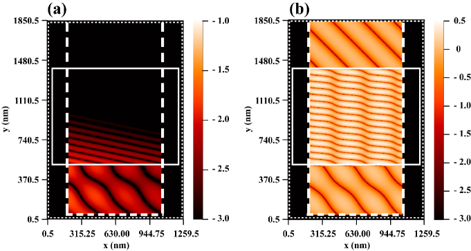
Figure 4: (color online) Magnetic field snapshots of a plane wave obliquely incident on a dielectric slab (indicated by a solid rectangle). Reflection and refraction (a) at the lower interface (at $10.01$ fs) and (b) after steady state is established (at $100.07$ fs). The incident plane wave enters the TF region from the lower left corner of the TF/SF boundary with incident angle $\theta=45^{\circ}$. The incident wavelength in vacuum is $\lambda=400$ nm (period $T=1.33$ fs), and the steady-state amplitude of the incident magnetic field is $1$ A/m in all calculations. The dielectric constant and thickness of the slab are $\epsilon_{r}=11.7$ and $900$ nm, respectively. The media above and below the slab are vacuum, the mesh size is $\Delta x=1.0$ nm, and the Courant number is $S=0.3$. A log color scale is used in all plots. The thick, dashed (thin, dotted) rectangle indicates the TF/SF (inner PML) boundary. The slab does not penetrate into the PML region.

As a second example, we study a plane wave obliquely incident on a dielectric slab.Winton ; Capoglu . In Fig. 4, we plot snapshots of the magnetic field of a plane wave (wavelength $400$ nm) incident at an angle $\theta=45^{\circ}$ on a $900$-nm thick dielectric slab (dielectric constant $\epsilon_{r}=11.7$). In both panels, the solid rectangle indicates the location of the slab, while the thick, dashed rectangle shows the TF/SF boundary. The plane wave is injected from the lower left corner and first impinges on the lower vacuum/dielectric interface. In panel (a), we observe the interference patterns of the reflected wave with the incident wave below the lower vacuum/dielectric interface while the refracted wave front propagates in the slab. The faint wave front in the dielectric slab is due to the slow Gaussian ramping of the incident field. After a steady state is established [Fig. 4(b)], the magnetic field pattern clearly reveals the interference between the reflected and incident waves, the interference within the dielectric slab, and the final transmission through the slab. In Fig. 4 (b), it is observed that the final transmitted wave maintains the same propagation direction as the incident wave ($45^{\circ}$ to $+y$ direction) because the media below and above the slab are both vacuum.

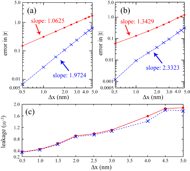
Figure 5: (color online) Relative error in the magnitude of (a) the reflection coefficient $r$ and (b) the transmission coefficient $t$ as a function of the mesh size $\Delta x$. (c) Maximum leakage as a function of mesh size $\Delta x$. In all calculations, the Courant number is $S=0.3$. In all figures, the red, solid (blue, dashed) curve shows the result without (with) the interface averaging of the dielectric constants. The parameters of the incident wave and the dielectric slab are as in the calculation leading to Fig. 4.

We proceed to examine the convergence of the magnitude of the reflection ($r$) and transmission ($t$) coefficients to the analytical results given by Eqs. (23) and (24). In Fig. 5, we plot the relative errors in (a) $|r|$ and (b) $|t|$ with respect to analytical results as a function of the mesh size $\Delta x$. The red, solid (blue, dashed) curve in Fig. 5 shows the convergence result without (with) the interface averaging of the dielectric constant. From the comparison, it is clear that calculations with interface correction lead to uniformly smaller error than that without the interface correction. The slope of each line in the log-log plot obtained by the least-square fit indicates that second order accuracy of Yee’s algorithm is maintained with the interface correction, while the accuracy degrades to first order without the interface correction. Similar effects have been reported in previous studies on the accuracy of FDTD results with dielectric interfaces,Hirono ; Hwang while here we observe such effects within the TF/SF formulation in the context of layered media. We note that the interface correction scheme does not entail additional computational and memory requirements and is thus always recommended. In Fig. 5 (c), we show that the maximum leakage with interface averaging is uniformly smaller than that without the interface averaging for different mesh sizes. Throughout, the maximum leakage is below $2.0\times 10^{-3}$, substantiating our confidence in the TF/SF scheme.Taflove

To further test the accuracy of the dielectric slab reflection and transmission upon oblique incidence of a plane wave, we compare the analytical results with FDTD calculated results at different incident wavelengths in Table 1 and at different incident angles in Table 2. As shown, the relative error (given in parentheses) is uniformly below $5\%$, except for incident angle $\theta=50^{\circ}$, where $|r|$ is below $0.01$. It is interesting to note that the relative error diminishes with increasing wavelength, while a non-monotonic trend is seen in the errors of both reflection and transmission coefficients for an increasing incident angle.

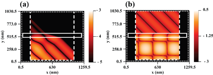
Figure 6: (color online) Magnetic field snapshots of a plane wave obliquely incident on a Drude metal slab (indicated by a solid rectangle). Reflection, refraction and transmission (a) before (at $2.50$ fs) and (b) after (at $60.04$ fs) steady state is established. In all calculations, the incident plane wave enters the TF region from the lower left corner of the TF/SF boundary (dashed lines) with incident angle $\theta=45^{\circ}$. The incident wavelength in vacuum is $\lambda=400$ nm (period $T=1.33$ fs), and the steady-state amplitude of the incident magnetic field is $1$ A/m. The metal slab is $80$ nm thick with Drude parameters: $\epsilon(\infty)=7.0246$, $\omega_{D}=1.5713\times 10^{16}$ rad/s, and $\Gamma_{D}=1.4003\times 10^{14}$ rad/s. The media above and below the slab are vacuum, the mesh size is $\Delta x=1.0$ nm, and the Courant number is $S=0.3$. A log color scale is used in all plots. The thick, dashed (thin, dotted) rectangle indicates the TF/SF (inner PML) boundary. The slab does not penetrate into the PML region.

Next we apply the TF/SF method to study the reflection and refraction of a plane wave obliquely incident upon a dispersive metal slab. Snapshots of the magnetic field are shown in Fig. 6 as the plane wave passes through the metal slab. Specifically, we consider an incident plane wave with wavelength $400$ nm and $\theta=45^{\circ}$ injected from the lower left corner of the TF region upon an $80$ nm thick dispersive metal slab described by the Drude model $\epsilon_{m}=\epsilon(\infty)-\omega_{D}^{2}/(\omega^{2}+i\Gamma_{D}\omega)$, with $\epsilon(\infty)=7.0246$, $\omega_{D}=1.5713\times 10^{16}$ rad/s, and $\Gamma_{D}=1.4003\times 10^{14}$ rad/s. This set of parameters is optimized to fit the dielectric data reported in Ref. Johnson, for bulk silver in the spectral range from $330$ to $500$ nm. Figures 6 (a) and (b) illustrate the magnetic field distribution before and after reaching a steady state, respectively. In Fig. 6 (b), the large curvatures at the interference minima between the incident and reflected fields below the lower interface indicate a large reflection coefficient ($>0.9$). Inside the metal, because of the complex dielectric function of the slab, the wave front is no longer a plane wave, as is clearly discernable in Fig. 6. However, the final transmitted wave exiting from the upper interface recovers a plane wave front and the same propagation constant as the incident wave, because the media below and above the dispersive slab are both vacuum. From Figs. 4(b) and 6(b), it is seen that the periodicity in the $x$ direction of the fields below, inside, and above the slab is the same. By further observing the field propagation after reaching the steady state in both cases (not shown), it is clear that the phase of the total field in the $x$ direction is matched. This observation confirms the phase matching condition parallel to the interface (same $k_{x}$ across the interfaces), which is critical to the derivation of the 1D field propagation, Eq. (6).

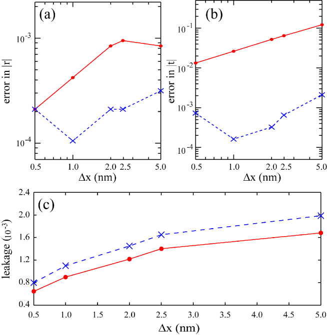
Figure 7: (color online) Relative error in the magnitude of the (a) the reflection coefficient $r$ and (b) the transmission coefficient $t$ as a function of the mesh size $\Delta x$. (c) Maximum leakage as a function of mesh size $\Delta x$. The Courant number is $S=0.3$ in all calculations. In all figures, the red, solid (blue, dashed) curve shows the result without (with) the interface averaging of the dielectric constants. The parameters of the incident wave and the metal slab are the same as in the calculations leading to of Fig. 6.

To examine the convergence of our results in the case of the metal slab, we use the same incident field condition as that in Fig. 6 and plot the relative error of the reflection and transmission coefficients as a function of the mesh size $\Delta x$ in Figs. 7 (a) and (b), respectively. It is seen that the results with interface averaging (blue, dashed curves) of the dielectric function yield uniformly lower error than the results without the interface averaging (red, solid curves). A first-order power law is seen in the error of the transmission coefficient as a function of the mesh size without interface averaging, all other errors are near and below $10^{-3}$, illustrating the convergence of the FDTD results. FDTD simulations on similar dispersive systems have been reported by Mohammodi et al., who suggested that the dispersive contour-path method is able to achieve smaller error even for a relatively large step-size ($\Delta x$).Mohammadi2 Fig. 7(c) shows that the leakage decreases with a decreasing mesh size, albeit in this case the leakage with the interface averaging of the dielectric function is slightly larger than that without the averaging [cf. Fig. 5(c)].

In Tables 3 and 4, we compare between the analytical and the FDTD calculated reflection and transmission coefficient magnitudes at various incident wavelengths and incident angles for the metal slab studied in Fig. 6. The FDTD results are obtained after steady state is reached under cw incident plane wave illumination. In the frequency domain, this corresponds to a fixed incident wavelength, and the Drude model provides a constant complex value of dielectric function, which can be used in Eqs. (23) and (24) to obtain the reflection and transmission coefficients. In Table 3, we list the free space wavelength in the $350$ to $500$ nm range, to which the fitted Drude model is applicable. The small relative errors ($<2.5\%$) shown in the parentheses in Tables 3 and 4 illustrates the reliability of our calculations using the TF/SF formulation in the case of layered dispersive media. The maximum leakage found in obtaining the data in Tables 3 and 4 is $1.201\times 10^{-2}$, which occurs at $\theta=80^{\circ}$.

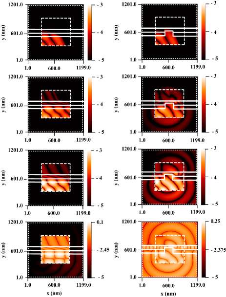
Figure 8: (color online) Magnetic field snapshots for a plane wave obliquely incident on two layers of materials. The interfaces between the layers and vacuum are indicated by solid horizontal lines. The lower layer is an $80$ nm thick Drude metal with parameters: $\epsilon(\infty)=7.0246$, $\omega_{D}=1.5713\times 10^{16}$ rad/s, and $\Gamma_{D}=1.4003\times 10^{14}$ rad/s. The upper layer is a $100$ nm dielectric with dielectric constant $\epsilon_{r}=11.7$. The media below and above the two layers are vacuum. The panels in the right column illustrate the scattering due to a slit of width $200$ nm and depth $120$ nm in the same layered structure as in the left column. Rows 1, 2, and 3 show snapshots at $1.60$, $3.20$, $4.80$ fs (before a steady state is established); Row 4 shows the snapshot at $60.04$ fs (after a steady state is established). For all calculations, the incident plane wave enters the TF region from the lower left corner of the TF/SF boundary with with incident angle $\theta=65^{\circ}$. The incidence wavelength is $\lambda=400$ nm (period $T=1.33$ fs), and the steady-state amplitude of the incident magnetic field is $1$ A/m. The mesh size is $\Delta x=2.0$ nm, and the Courant number is $S=0.3$. A log color scale is used in all plots. The thick, dashed (thin, dotted) rectangle indicates the TF/SF (inner PML) boundary. The slabs are extended into the UPML region.

Panels in the left column of Fig. 8 illustrate snapshots of the magnetic field as the wave propagates through two-layer media consisting of a lower layer of $80$-nm thick dispersive material and an upper layer of $100$-nm thick dielectric material under oblique plane wave incidence. The material parameters are given in the caption of Fig. 8. In these panels, the solid horizontal lines define the boundaries between different layers, which are extended into the UPML in the $x$ direction. The dashed box denotes the TF/SF boundary. The incident plane wave with wavelength $400$ nm and $\theta=65^{\circ}$ is injected from the lower left corner of the TF region. The magnetic field snapshots in the first column of Fig. 8 show that Snell’s law is obeyed when the field passes through the two layers of materials. In particular, the propagation direction in the high-index dielectric material exhibits a smaller angle to the normal than the incident wave, whereas the final transmitted wave propagates along the direction of the incident wave. More importantly, we observe that the phase of the waves across the different layers is matched in the $x$ direction after a steady state is established (bottom panel in the left column), which is again consistent with Eq. (6). In this case, the magnitude of the reflection and transmission coefficients calculated by FDTD is $|r|=0.9524$ and $|t|=0.0866$, respectively. The bottom panel in the left column also shows non-negligible leakage penetrating through the TF/SF box and propagating into the lower right corner of the simulation domain, nevertheless, the maximum value of the leakage in $H_{z}$ is $1.5461\times 10^{-4}$, which is insignificant in practice.

Panels in the second column of Fig. 8 are obtained under the same conditions as those in the first column except that a slit of $200$ nm width (in the $x$ direction) and $120$ nm depth (in the $y$ direction) is placed in the middle of the simulation domain. In the TF region, the slit causes strong scattering of the injected plane wave, which results in the observed interference patterns. The slit introduces entirely new physics: outside the TF/SF boundary, the purely scattered wave distribution is reminiscent of a dipole radiation pattern. Closer inspection reveals that the field distribution is asymmetric with respect to the slit center ($x=600$ nm). The scattered field is strongest near the lower surface of the dispersive slab and to the right of the TF/SF box and weakest above the upper surface of the dielectric slab and to the left of the TF/SF box. The asymmetric angular distribution is a clear signature of the oblique incidence of the exciting plane wave. By enlarging the SF region size, we find that the purely scattered wave along the lower surface of the metal thin film consists mainly of surface plasmon polariton (SPP) waves propagating away from the slit. These are identified by their wavelength - $~{}348$ nm in the $x$ direction compared with the analytical result for the wavelength of SPP at the interface between vacuum and metal, which is given by $\lambda_{0}/\rm{Re}\sqrt{\epsilon_{m}/(1+\epsilon_{m})}=348.25$ nm.

For the simulations in Fig. 8, we have updated the field at the horizontal and vertical interfaces using the averaging scheme discussed above, and have tested the convergence of the fields in the TF and SF regions with respect to mesh size ($\Delta x$), TF box size, and physical size of the simulation region. We note that UPML termination of the simulation domain is important because the scattered field due to the slit is significant. Our tests show that the maximum scattered field in the SF region is only one order of magnitude less than the maximum field in the TF region. Additionally, the UPML can effectively absorb the outgoing wave in the dispersive and dielectric layers. Furthermore, the boxed TF/SF boundary has advantage over the $\Pi$-shaped boundary considered previously, particularly when one is interested in the full angular distribution of the scattered field in the far-field zone.

IV Conclusions

Using Maxwell’s equations for the transverse magnetic wave, along with translational invariance and phase matching principles, we derived an equivalent one-dimensional wave propagation equation along the direction perpendicular to the interfaces between layered media. We then derived the corresponding finite-difference time-domain equations for layered dielectric media and dispersive media with a Drude pole pair. To utilize these equations for a plane wave with oblique incidence, we discussed the simulation setup and procedure in the framework of the total field / scattered field formulation with a special emphasis on techniques to match the fields at the total field / scattered field boundary. We have performed tests on vacuum propagation and on the reflection and refraction at a dielectric and a dispersive slab. Converged simulation results for various incident angles and wavelengths reveal that the errors in the reflection and refraction coefficients are uniformly below $5\%$ compared to analytic results. The numerical example of scattering at a nano-scale (sub-wavelength) slit in a dispersive medium invites interesting applications of our formulation to time-dependent studies of electromagnetic wave scattering at surface or embedded scatters in dispersive media, for example, the coupling of incident oblique plane wave into surface plasmon polaritons. For this purpose, the developed method offers the flexibility of choosing the total field region inside which the near-field exhibits interference pattern between incident and scattered fields, while outside which the scattered far-field can be detected at all angles.

Appendix A TE mode wave propagation

Maxwell’s equations in 2D in the frequency domain for the TE mode read,

$$\frac{\partial H_{y}}{\partial x}-\frac{\partial H_{x}}{\partial y}=-i\omega\epsilon_{0}\epsilon(\omega)E_{z},$$ (31)

$$\frac{\partial E_{z}}{\partial y}=i\omega\mu_{0}H_{x},$$ (32)

$$\frac{\partial E_{z}}{\partial x}=-i\omega\mu_{0}H_{y}.$$ (33)

Substituting Eq. (33) into Eq. (31) yields,

$$\frac{\partial H_{x}}{\partial y}=i\omega\epsilon_{0}\left[\epsilon(\omega)-\epsilon_{1r}\sin^{2}(\theta)\right]E_{z},\\$$ (34)

where $\epsilon_{1r}$ denotes the relative permitivity of the first medium (see Fig. 1). Equations (32) and (33) are used for 1D TE mode wave propagation. These equations can be readily solved using the same FDTD procedure as for Eqs. (2) and (3). The time-domain solution is facilitated by the fact that material dispersiveness introduces a factor $\left[\epsilon(\omega)-\epsilon_{1r}\sin^{2}(\theta)\right]$ in Eq. (34), whereas in Eq. (6) it introduces a factor $\left[\epsilon(\omega)-\epsilon_{1r}\sin^{2}(\theta)\right]/\epsilon(\omega)$, which entails more difficulty for the FDTD solution.footnote3 The simulation setup and flow chart in Section II can be used for the TE mode by exchanging the roles of the $E$ and $H$ fields.

Appendix B FDTD equations for 2D TM mode wave propagation

The FDTD equations based on the auxiliary differential equation (ADE) approach read,

$$E_{x}|^{n+1}_{i+1/2,j} = a_{x1}E_{x}|^{n}_{i+1/2,j}+a_{x2}(H_{zy}|^{n+1/2}_{i+1/2,j+1/2}-H_{zy}|^{n+1/2}_{i+1/2,j-1/2})+a_{x3}J_{x}|^{n+1/2}_{i+1/2,j},$$ (35)

$$J_{x}|^{n+3/2}_{i+1/2,j} = a_{x4}J_{x}|^{n+1/2}_{i+1/2,j}+a_{x5}E_{x}|^{n+1}_{i+1/2,j},$$ (36)

$$E_{y}|^{n+1}_{i,j+1/2} = a_{y1}E_{y}|^{n}_{i,j+1/2}+a_{y2}(H_{zx}|^{n+1/2}_{i+1/2,j+1/2}-H_{zx}|^{n+1/2}_{i-1/2,j+1/2})+a_{y3}J_{y}|^{n+1/2}_{i,j+1/2},$$ (37)

$$J_{y}|^{n+3/2}_{i,j+1/2} = a_{y4}J_{y}|^{n+1/2}_{i,j+1/2}+a_{y5}E_{y}|^{n+1}_{i,j+1/2},$$ (38)

$$H_{zx}|^{n+3/2}_{i+1/2,j+1/2} = b_{x1}H_{zx}|^{n+1/2}_{i+1/2,j+1/2}+b_{x2}(E_{y}|^{n+1}_{i+1,j+1/2}-E_{y}|^{n+1}_{i,j+1/2}),$$ (39)

$$H_{zy}|^{n+3/2}_{i+1/2,j+1/2} = b_{y1}H_{zy}|^{n+1/2}_{i+1/2,j+1/2}+b_{y2}(E_{x}|^{n+1}_{i+1/2,j+1}-E_{x}|^{n+1}_{i+1/2,j}),$$ (40)

$$H_{z} = H_{zx}+H_{zy}.$$ (41)

The coefficients in the $E$-field updating equations are medium dependent; specifically, in vacuum ($\epsilon_{r}=1$) and dielectric media (constant $\epsilon_{r}$),Taflove

$$\begin{cases}a_{x1}=a_{y1}=1,\\ a_{x2}=-a_{y2}=\Delta t/(\epsilon_{0}\epsilon_{r}\Delta x),\\ a_{x3}=a_{x4}=a_{x5}=a_{y3}=a_{y4}=a_{y5}=0,\end{cases}$$ (42)

in Drude media, $\epsilon_{m}=\epsilon(\infty)-\omega_{D}^{2}/(\omega^{2}+i\Gamma_{D}\omega)$,Gray

$$\begin{cases}a_{x1}=a_{y1}=1,\\ a_{x2}=-a_{y2}=\Delta t/\left[\epsilon_{0}\epsilon(\infty)\Delta x\right],\\ a_{x3}=a_{y3}=-\Delta t/\left[\epsilon_{0}\epsilon(\infty)\right],\\ a_{x4}=a_{y4}=(1-\Gamma_{D}\Delta t)/(1+\Gamma_{D}\Delta t),\\ a_{x5}=a_{y5}=\epsilon_{0}\omega_{D}^{2}\Delta t/(1+\Gamma_{D}\Delta t),\end{cases}$$ (43)

and in the PML region,

$$\begin{cases}a_{x1}=\exp(-\sigma_{y}\Delta t/\epsilon_{0}),\\ a_{x2}=\left[1-\exp(-\sigma_{y}\Delta t/\epsilon_{0})\right]/(\Delta x\sigma_{y}),\\ a_{x3}=a_{x4}=a_{x5}=0;\\ a_{y1}=\exp(-\sigma_{x}\Delta t/\epsilon_{0}),\\ a_{y2}=-\left[1-\exp(-\sigma_{x}\Delta t/\epsilon_{0})\right]/(\Delta x\sigma_{x}),\\ a_{y3}=a_{y4}=a_{y5}=0.\end{cases}$$ (44)

The coefficients in the $H$-field updating equations outside the PML regions are,

$$\begin{cases}b_{x1}=b_{y1}=1,\\ b_{x2}=-b_{y2}=-\Delta t/(\mu_{0}\Delta x),\end{cases}$$ (45)

whereas in the PML regions they read,

$$\begin{cases}b_{x1}=\exp(-\sigma^{*}_{x}\Delta t/\mu_{0}),\\ b_{x2}=-\left[1-\exp(-\sigma^{*}_{x}\Delta t/\mu_{0})\right]/(\Delta x\sigma^{*}_{x}),\\ b_{y1}=\exp(-\sigma^{*}_{y}\Delta t/\mu_{0}),\\ b_{y2}=\left[1-\exp(-\sigma^{*}_{y}\Delta t/\mu_{0})\right]/(\Delta x\sigma^{*}_{y}).\end{cases}$$ (46)

Here, we assume a polynomial grading of the PML parameters:Taflove $\sigma_{x,y}=\epsilon_{0}\sigma^{*}_{x,y}/\mu_{0}=\sigma_{m}(\rho/\delta)^{m}$, where $\sigma_{m}$ is the maximum conductance in the PML, $\rho$ is the distance into the PML, and $\delta$ is the thickness of the PML region. In this paper, we use a power $m=4$ and $\delta=20\Delta x$. $\sigma_{m}$ is optimized to give a maximum reflection error on the order of $10^{-7}$.

The FDTD equations based on the UPML formulation read,Gedney

$$P_{x}|^{n+1}_{i+1/2,j} = P_{x}|^{n}_{i+1/2,j}+\alpha_{x1}(H_{z}|^{n+1/2}_{i+1/2,j+1/2}-H_{z}|^{n+1/2}_{i+1/2,j-1/2}),$$ (47)

$$D_{x}|^{n+1}_{i+1/2,j} = \alpha_{x2}D_{x}|^{n}_{i+1/2,j}+\alpha_{x3}D_{x}|^{n-1}_{i+1/2,j}+\alpha_{x4}P_{x}|^{n+1}_{i+1/2,j}$$ (48)

$$+\alpha_{x5}P_{x}|^{n}_{i+1/2,j}+\alpha_{x6}P_{x}|^{n-1}_{i+1/2,j},$$

$$E_{x}|^{n+1}_{i+1/2,j} = \alpha_{x7}E_{x}|^{n}_{i+1/2,j}+\alpha_{x8}\alpha_{x9}D_{x}|^{n+1}_{i+1/2,j}+\alpha_{x8}\alpha_{x10}D_{x}|^{n}_{i+1/2,j},$$ (49)

$$P_{y}|^{n+1}_{i,j+1/2} = P_{y}|^{n}_{i,j+1/2}+\alpha_{y1}(H_{z}|^{n+1/2}_{i+1/2,j+1/2}-H_{z}|^{n+1/2}_{i-1/2,j+1/2}),$$ (50)

$$D_{y}|^{n+1}_{i,j+1/2} = \alpha_{y2}D_{y}|^{n}_{i,j+1/2}+\alpha_{y3}D_{y}|^{n-1}_{i,j+1/2}+\alpha_{y4}P_{y}|^{n+1}_{i,j+1/2}$$ (51)

$$+\alpha_{y5}P_{y}|^{n}_{i,j+1/2}+\alpha_{y6}P_{y}|^{n-1}_{i,j+1/2},$$

$$E_{y}|^{n+1}_{i,j+1/2} = \alpha_{y7}E_{y}|^{n}_{i,j+1/2}+\alpha_{y8}\alpha_{y9}D_{y}|^{n+1}_{i,j+1/2}+\alpha_{y8}\alpha_{y10}D_{y}|^{n}_{i,j+1/2},$$ (52)

$$B_{z}|^{n+3/2}_{i+1/2,j+1/2} = \beta_{1}B_{z}|^{n+1/2}_{i+1/2,j+1/2}$$ (53)

$$+\beta_{2}(E_{y}|^{n+1}_{i+1,j+1/2}-E_{y}|^{n+1}_{i,j+1/2}-E_{x}|^{n+1}_{i+1/2,j}+E_{x}|^{n+1}_{i+1/2,j+1}),$$

$$H_{z}|^{n+3/2}_{i+1/2,j+1/2} = \beta_{3}H_{z}|^{n+1/2}_{i+1/2,j+1/2}+\beta_{4}(B_{z}|^{n+3/2}_{i+1/2,j+1/2}-B_{z}|^{n+1/2}_{i+1/2,j+1/2}).$$ (54)

The coefficients in the $E$-field updating equations in all media are,

$$\alpha_{x1}=-\alpha_{y1}=\Delta t/\Delta x.$$ (55)

In vacuum ($\epsilon_{r}=1$) and dielectric media (constant $\epsilon_{r}$),

$$\begin{cases}\alpha_{x2}=\alpha_{x3}=\alpha_{x5}=\alpha_{x6}=\alpha_{y2}=\alpha_{y3}=\alpha_{y5}=\alpha_{y6}=0,\\ \alpha_{x4}=\alpha_{y4}=1/\epsilon_{r},\end{cases}$$ (56)

whereas in Drude media,

$$\begin{cases}\alpha_{x2}=\alpha_{y2}=\frac{4\epsilon(\infty)}{2\epsilon(\infty)+\epsilon(\infty)\Gamma_{D}\Delta t+\omega_{D}^{2}\Delta t^{2}},\\ \alpha_{x3}=\alpha_{y3}=\frac{-2\epsilon(\infty)+\epsilon(\infty)\Gamma_{D}\Delta t-\omega_{D}^{2}\Delta t^{2}}{2\epsilon(\infty)+\epsilon(\infty)\Gamma_{D}\Delta t+\omega_{D}^{2}\Delta t^{2}},\\ \alpha_{x4}=\alpha_{y4}=\frac{2+\Gamma_{D}\Delta t}{2\epsilon(\infty)+\epsilon(\infty)\Gamma_{D}\Delta t+\omega_{D}^{2}\Delta t^{2}},\\ \alpha_{x5}=\alpha_{y5}=\frac{-4}{2\epsilon(\infty)+\epsilon(\infty)\Gamma_{D}\Delta t+\omega_{D}^{2}\Delta t^{2}},\\ \alpha_{x6}=\alpha_{y6}=\frac{2-\Gamma_{D}\Delta t}{2\epsilon(\infty)+\epsilon(\infty)\Gamma_{D}\Delta t+\omega_{D}^{2}\Delta t^{2}}.\\ \end{cases}$$ (57)

outside the UPML regions,

$$\begin{cases}\alpha_{x7}=\alpha_{x9}=\alpha_{x10}=\alpha_{x7}=\alpha_{x9}=\alpha_{x10}=1,\\ \alpha_{x8}=\alpha_{y8}=1/\epsilon_{0},\\ \end{cases}$$ (58)

and in the UPML regions,

$$\begin{cases}\alpha_{x7}=\frac{2\epsilon_{0}\kappa_{y}-\sigma_{y}\Delta t}{2\epsilon_{0}\kappa_{y}+\sigma_{y}\Delta t},\\ \alpha_{x8}=\frac{1}{2\epsilon_{0}^{2}\kappa_{y}+\epsilon_{0}\sigma_{y}\Delta t},\\ \alpha_{x9}=\sigma_{x}\Delta t+2\epsilon_{0}\kappa_{x},\\ \alpha_{x10}=\sigma_{x}\Delta t-2\epsilon_{0}\kappa_{x},\\ \alpha_{y7}=\frac{2\epsilon_{0}\kappa_{x}-\sigma_{x}\Delta t}{2\epsilon_{0}\kappa_{x}+\sigma_{x}\Delta t},\\ \alpha_{y8}=\frac{1}{2\epsilon_{0}^{2}\kappa_{x}+\epsilon_{0}\sigma_{x}\Delta t},\\ \alpha_{y9}=\sigma_{y}\Delta t+2\epsilon_{0}\kappa_{y},\\ \alpha_{x10}=\sigma_{y}\Delta t-2\epsilon_{0}\kappa_{y}.\end{cases}$$ (59)

The coefficients in the $H$-field updating equations outside the UPML region are,

$$\begin{cases}\beta_{1}=\beta_{3}=1,\\ \beta_{2}=\Delta t/\Delta x,\\ \beta_{4}=1/\mu_{0},\end{cases}$$ (60)

and in the UPML regions,

$$\begin{cases}\beta_{1}=\frac{2\epsilon_{0}\kappa_{x}-\sigma_{x}\Delta t}{2\epsilon_{0}\kappa_{x}+\sigma_{x}\Delta t},\\ \beta_{2}=-\frac{2\epsilon_{0}\Delta t}{(2\epsilon_{0}\kappa_{x}+\sigma_{x}\Delta t)\Delta x},\\ \beta_{3}=\frac{2\epsilon_{0}\kappa_{y}-\sigma_{y}\Delta t}{2\epsilon_{0}\kappa_{y}+\sigma_{y}\Delta t},\\ \beta_{4}=\frac{2\epsilon_{0}}{(2\epsilon_{0}\kappa_{y}+\sigma_{y}\Delta t)\mu_{0}}.\end{cases}$$ (61)

Here, we assume a polynomial grading of the PML parameters,Taflove $\sigma_{x,y}=\sigma_{m}(\rho/\delta)^{m}$ and $\kappa_{x,y}=1+(\kappa_{m}-1)(\rho/\delta)^{m}$, where $\sigma_{m}$ and $\kappa_{m}$ denote the maxima of the UPML parameters $\rho$ is distance into the PML, and $\delta$ is the thickness of the PML. In this paper, we use power $m=4$, $\delta=20\Delta x$, $\kappa_{m}=1$, and $\sigma_{m}$ is optimized to give a maximum reflection error on the order of $10^{-7}$ for a simulation region consisting of vacuum and on the order of $10^{-4}$ for a simulation region consisting of Drude dispersive media.

Appendix C Systematic solution of one-dimensional wave propagation in the TM mode

In this appendix we provide a systematic solution for Eq. (8) when $0<\sin(\theta)<1$ and $\epsilon(\omega)$ consists of a linear superposition of Debye, Drude, and Lorentz types of poles. In this case, we first rearrange Eq. (8) as

$$\epsilon_{1r}\sin^{2}(\theta)H_{z}=\epsilon(\omega)(H_{z}-H^{\prime}_{z}),$$ (62)

where

$$\epsilon(\omega)=\epsilon(\infty)+\displaystyle\sum_{i}\epsilon_{i}(\omega),$$ (63)

andTaflove

$$\epsilon_{i}(\omega)=\begin{cases}\epsilon_{DB}(\omega)=\frac{\Delta\epsilon_{DB}}{1-i\omega\tau_{DB}},&\text{for a Debye pole}\\ \epsilon_{DR}(\omega)=-\frac{\omega^{2}_{DR}}{\omega^{2}+i\Gamma_{DR}\omega},&\text{for Drude pole pairs}\\ \epsilon_{L}(\omega)=-\frac{\Delta\epsilon_{L}\omega^{2}_{L}}{\omega^{2}-\omega^{2}_{L}+i2\Gamma_{L}\omega},&\text{for Lorentz pole pairs.}\\ \end{cases}$$ (64)

We introduce auxiliary variables $K_{i}$ to rewrite Eq. (62) as a system of equations,

$$\epsilon_{1r}\sin^{2}(\theta)H_{z} = K_{0}+\displaystyle\sum_{i}K_{i},$$ (65)

$$K_{0} = \epsilon(\infty)(H_{z}-H^{\prime}_{z}),$$ (66)

$$K_{i} = \epsilon_{i}(\omega)(H_{z}-H^{\prime}_{z}).$$ (67)

Equations (65) and (66) correspond to the set of FDTD equations,

$$\epsilon_{1r}\sin^{2}(\theta)H_{z}|^{n+3/2}-K_{0}|^{n+3/2}-\displaystyle\sum_{i}K_{i}|^{n+3/2}=0,$$ (68)

$$\epsilon(\infty)H_{z}|^{n+3/2}-K_{0}|^{n+3/2}=\epsilon(\infty)H^{\prime}_{z}|^{n+3/2}.$$ (69)

The translation of Eq. (67) into a set of FDTD equations depends on the type of pole(s) considered [see Eq. (64)]. For a single Debye pole ($K_{i}=K_{DB}$),

$$\Delta\epsilon_{DB}\Delta tH_{z}|^{n+3/2}-(2\tau_{DB}+\Delta t)K_{DB}|^{n+3/2}$$

$$=(\Delta t-2\tau_{DB})K_{DB}|^{n+1/2}$$

$$+\Delta\epsilon_{DB}\Delta t(H^{\prime}_{z}|^{n+3/2}+H^{\prime}_{z}|^{n+1/2}-H_{z}|^{n+1/2}).$$ (70)

For a Drude pole pair ($K_{i}=K_{DR}$),

$$\omega^{2}_{DR}\Delta t^{2}H_{z}|^{n+3/2}-(\Gamma_{DR}\Delta t+2)K_{DR}|^{n+3/2}$$

$$=-4K_{DR}|^{n+1/2}+(2-\Gamma_{DR}\Delta t)K_{DR}|^{n-1/2}$$

$$+\omega^{2}_{DR}\Delta t^{2}(H^{\prime}_{z}|^{n+3/2}+H^{\prime}_{z}|^{n-1/2}-H_{z}|^{n-1/2}).$$ (71)

For a Lorentz pole pair ($K_{i}=K_{L}$),

$$\Delta\epsilon_{L}\omega^{2}_{L}\Delta t^{2}H_{z}|^{n+3/2}-(\omega^{2}_{L}\Delta t^{2}+2\Gamma_{L}\Delta t+2)K_{L}|^{n+3/2}$$

$$=-4K_{L}|^{n+1/2}+(\omega^{2}_{L}\Delta t^{2}-2\Gamma_{L}\Delta t+2)K_{L}|^{n-1/2}$$

$$+\Delta\epsilon_{L}\omega^{2}_{L}\Delta t^{2}(H^{\prime}_{z}|^{n+3/2}+H^{\prime}_{z}|^{n-1/2}-H_{z}|^{n-1/2}).$$ (72)

Equations (68) through (72) form a linear system of equations for the unknowns $H_{z}|^{n+3/2}$ and $K_{i}|^{n+3/2}$ ($i=0,1,...$), which can be solved by existing numerical solvers for linear systems of equations. The solution is then used to replace Eq. (12) to proceed the 1D wave propagation for the TM mode Comparing to a direct Fourier transform of Eq. (6), the above procedure only requires the storage of the quantities at the previous two time instances and thus avoids the complexity of numerical high-order derivatives with respect to time. This procedure can be extended systematically to multi-poles in the material dispersiveness, although it involves solving a linear system of equations.

FIGURES

TABLES

Table 1: Comparison of the magnitude of the reflection ($r$) and transmission ($t$) coefficients between the analytical and numerical results for different incidence wavelengths ($\lambda$). Superscript $a$ denotes the analytical, and superscript $n$ denotes the numerical results. The percentages in brackets denote the relative errors in the numerical results. The mesh size is $\Delta x=1$ nm and the Courant number is $S=0.3$.

$\lambda$ (nm)	$|r^{a}|$	$|r^{n}|$(error)	$|t^{a}|$	$|t^{n}|$(error)
$300$	$0.2485$	$0.2600(4.63\%)$	$0.9686$	$0.9658(0.29\%)$
$400$	$0.1898$	$0.1949(2.69\%)$	$0.9818$	$0.9809(0.09\%)$
$500$	$0.1532$	$0.1558(1.70\%)$	$0.9882$	$0.9878(0.04\%)$
$600$	$0.1282$	$0.1298(1.25\%)$	$0.9912$	$0.9916(0.04\%)$
$700$	$0.6990$	$0.6988(0.03\%)$	$0.7152$	$0.7154(0.03\%)$
$800$	$0.7172$	$0.7171(0.01\%)$	$0.6969$	$0.6969(<0.02\%)$

Table 2: Comparison of the magnitude of the reflection ($r$) and transmission ($t$) coefficients between the analytical and numerical results for different incidence angles ($\theta$) and Courant numbers ($S$). Results are obtained for a plane wave with $400$ nm wavelength incident upon a $900$ nm thick dielectric slab ($\epsilon_{r}=11.7$). Superscript $a$ denotes the analytical, and superscript $n$ denotes the numerical results. The percentages in brackets denote the relative errors in the numerical results. The mesh size is $\Delta x=1$ nm.

$\theta$ (degree)	$S$	$|r^{a}|$	$|r^{n}|$(error)	$|t^{a}|$	$|t^{n}|$(error)
$0$	$0.3$	$0.8278$	$0.8281(0.04\%)$	$0.5610$	$0.5539(1.27\%)$
$10$	$0.1$	$0.8169$	$0.8174(0.06\%)$	$0.5767$	$0.5760(0.12\%)$
$20$	$0.2$	$0.7737$	$0.7747(0.13\%)$	$0.6335$	$0.6323(0.21\%)$
$30$	$0.3$	$0.6565$	$0.6588(0.35\%)$	$0.7543$	$0.7526(0.23\%)$
$40$	$0.3$	$0.3839$	$0.3884(1.17\%)$	$0.9234$	$0.9216(0.19\%)$
$50$	$0.3$	$0.0039$	$0.0089(128\%)$	$1.0000$	$1.0000(<0.01\%)$
$60$	$0.3$	$0.1981$	$0.1952(1.46\%)$	$0.9802$	$0.9808(0.06\%)$
$70$	$0.2$	$0.1152$	$0.1142(0.87\%)$	$0.9933$	$0.9935(0.02\%)$
$80$	$0.1$	$0.3395$	$0.3367(0.82\%)$	$0.9406$	$0.9470(0.68\%)$

Table 3: As in Table 1 for oblique incidence upon an $80$ nm thick silver slab. The Dielectric function of silver is described by the Drude model, $\epsilon_{m}=\epsilon(\infty)-\omega_{D}^{2}/(\omega^{2}+i\Gamma_{D}\omega)$, with $\epsilon(\infty)=7.0246$, $\omega_{D}=1.5713\times 10^{16}$ rad/s, and $\Gamma_{D}=1.4003\times 10^{14}$ rad/s. The mesh size is $\Delta x=5$ nm and the Courant number is $S=0.3$, except for the $\lambda=350$ nm case, where $\Delta x=2$ nm and the Courant number is $S=0.1$.

$\lambda$ (nm)	$|r^{a}|$	$|r^{n}|$(error)	$|t^{a}|$	$|t^{n}|$(error)
$350$	$0.8908$	$0.8908(<0.01\%)$	$0.2295$	$0.2295(<0.04\%)$
$400$	$0.9503$	$0.9500(0.03\%)$	$0.1231$	$0.1234(0.24\%)$
$450$	$0.9672$	$0.9672(<0.01\%)$	$0.0760$	$0.0761(0.13\%)$
$500$	$0.9743$	$0.9742(0.01\%)$	$0.0532$	$0.0533(0.19\%)$

Table 4: As in Table 2 for oblique incidence upon an $80$ nm thick silver slab. The dielectric function of silver is described by the Drude model, $\epsilon_{m}=\epsilon(\infty)-\omega_{D}^{2}/(\omega^{2}+i\Gamma_{D}\omega)$, with $\epsilon(\infty)=7.0246$, $\omega_{D}=1.5713\times 10^{16}$ rad/s, and $\Gamma_{D}=1.4003\times 10^{14}$ rad/s. The mesh size is $\Delta x=5$ nm.

$\theta$ (degree)	$S$	$|r^{a}|$	$|r^{n}|$(error)	$|t^{a}|$	$|t^{n}|$(error)
$0$	$0.3$	$0.9602$	$0.9592(0.10\%)$	$0.1202$	$0.1201(0.08\%)$
$10$	$0.1$	$0.9597$	$0.9596(0.01\%)$	$0.1204$	$0.1204(<0.08\%)$
$20$	$0.2$	$0.9580$	$0.9581(0.01\%)$	$0.1209$	$0.1210(<0.08\%)$
$30$	$0.3$	$0.9554$	$0.9560(0.06\%)$	$0.1218$	$0.1220(0.16\%)$
$40$	$0.3$	$0.9520$	$0.9520(<0.01\%)$	$0.1228$	$0.1230(0.16\%)$
$50$	$0.3$	$0.9488$	$0.9498(0.11\%)$	$0.1230$	$0.1234(0.33\%)$
$60$	$0.3$	$0.9478$	$0.9475(0.03\%)$	$0.1192$	$0.1197(0.42\%)$
$70$	$0.2$	$0.9532$	$0.9531(0.01\%)$	$0.1043$	$0.1048(0.48\%)$
$80$	$0.1$	$0.9711$	$0.9627(0.87\%)$	$0.0682$	$0.0665(2.49\%)$

References

- (1) J. D. Jackson, Classical Electrodynamics, 3rd ed. (John Wiley & Sons, New Jersey, 1998).
- (2) M. Born and E. Wolf, Principles of Optics, 6th ed. (Pergamon Press, Oxford, 1980).
- (3) J. Hecht, Understanding Fiber Optics, 5th ed. (Prentice Hall, New Jersey, 2005).
- (4) Ground Penetrating Radar: Theory and Applications, edited by H. M. Jol (Elsevier Science, Oxford, 2009).
- (5) A. Vander Vorst, A. Rosen, and Y. Kotsuka, RF/Microwave Interaction With Biological Tissues, (John Wiley & Sons, New Jersey, 2006).
- (6) W. L. Barnes, A. Dereux, and T. W. Ebbesen, Nature 424, 824 (2003).
- (7) E. Ozbay, Science 311, 189 (2006).
- (8) F. López-Tejeira, Sergio G. Rodrigo, L. Martín-Moreno, F. J. García-Vidal, E. Devaux, W. Ebbesen, J. R. Krenn, I. P. Radko, S. I. Bozhevolnyi, M. U. González., J. C. Weeber, and A. Dereux, Nat. Phys. 3, 324 (2007).
- (9) J. V. Coe, J. M. Heer, S. Teeters-Kennedy, H. Tian, and K. R. Rodriguez, Annu. Rev. Phys. Chem. 59, 179 (2008).
- (10) L. Yin, V. K. Vlasko-Vlasov, A. Rydh, J. Pearson, U. Welp, S.-H. Chang, S. K. Gray, G. C. Schatz, D. B. Brown, and C. W. Kimball, Appl. Phys. Lett. 85, 467 (2004).
- (11) Z. Liu, J. M. Steel, H. Lee, and X. Zhang, Appl. Phys. Lett. 88, 171108 (2006).
- (12) L. Douillard, F. Charra, Z. Korczak, R. Bachelot, S. Kostcheev, G. Lerondel, P.-M. Adam, and P. Royer, Nano Lett. 8, 935 (2008).
- (13) B. Wang, L. Aigouy, E. Bourhis, J. Gierak, J. P. Hugonin, and P. Lalanne, Appl. Phys. Lett. 94, 011114 (2009).
- (14) J. Renger, R. Quidant, N. van Hulst, S. Palomba, and L. Novotny, Phys. Rev. Lett. 103, 266802 (2009).
- (15) J. Bravo-Abad, L. Martín-Moreno, and F. J. García-Vidal, Phys. Rev. E, 69, 026601, (2004).
- (16) F. J. García-Vidal, E. Moreno, J. A. Porto, and L. Martín-Moreno, Phys. Rev. Lett. 95, 103901 (2005).
- (17) R. Gordon, Phys. Rev. B 75, 193401 (2007).
- (18) P. Lalanne, J. P. Hugonin, and J. C. Rodier, J. Opt. Soc. Am. A 23, 1608 (2006).
- (19) H. Kim and B. Lee, Plasmonics 4, 153 (2009).
- (20) K. F. MacDonald, Z. L. Sámson, M. I. Stockman, and N. Zheludev, Nat. Photonics 3, 55 (2009).
- (21) For a review, see A. Kubo, Y. S. Jung, H. K. Kim and H. Petek, J. Phys. B: At. Mol. Opt. Phys. 40, S259 (2007) and references therein.
- (22) We note that an obliquely incident beam in the finite-difference time-domain method has been developed previously. See, e.g., T.-W. Lee and S. K. Gray, Appl. Phys. Lett. 86, 141105 (2005); K. J. Willis, J. B. Schneider, and S. C. Hagness, Opt. Exp. 16, 1903 (2008). However, we stress that in these formulations the incident beam wave front is spatially non-uniform, in contrast to the formulation in this paper.
- (23) A. Taflove and S. C. Hagness, Computational Electrodynamics: The Finite-Difference Time-Domain Method, 3rd ed. (Artech House, Boston, 2005).
- (24) F. L. Teixeira, IEEE Trans. Antennas Propag. 56, 2150 (2008).
- (25) B. Ung and Y. Sheng, Opt. Exp. 15, 1182 (2007).
- (26) T.-W. Lee and S. Gray, Opt. Exp. 13, 9652 (2005).
- (27) S. C. Winton, P. Kosmas, and C. M. Rappaport, IEEE Trans. Antennas Propag. 53, 1721 (2005).
- (28) İ. R. Çapoǧlu and G. S. Smith, IEEE Trans. Antennas Propag. 56, 158 (2008).
- (29) Y.-N. Jiang, D.-B. Ge, and S.-J. Ding, Prog. Electromagn. Res. 83, 157 (2008).
- (30) H. Raether, Surface Plasmons (Springer, Berlin, 1988).
- (31) J.-P. Berenger, J. Comput. Phys. 114, 185 (1994).
- (32) S. D. Gedney, Electromagnetics 16, 399 (1996).
- (33) We note that, when incoporated with the Convolutional Perfectly Matched Layers absorbing boundary conditions, the ADE approach can systematically treat a general dispersive medium with a finite sum of Debye-, Lorentz- and Drude-type poles, while the UPML approach with higher order poles becomes increasingly difficult because of higher-order derivatives with respect to time. However, for a single Drude pole considered in this paper, the UPML approach is numerically tractable.
- (34) See Chap. 13 of Ref. Wolf, , Refs. Winton, , Capoglu, , and W. C. Chew, Waves and Fields in Inhomogeneous Media, (Van Nostrand Reinhold, New York, 1990), Chap. 2.
- (35) Y. Zhao and Y. Hao, IEEE Trans. Antennas Propag. 55, 3070 (2007).
- (36) A. Mohammadi and M. Agio, Opt. Exp. 14, 11330 (2006).
- (37) T. Hirono, Y. Shibata, W. W. Lui, S. Seki, and Y. Yoshikuni, IEEE Microwave Guided Wave Lett., 10, 359 (2000).
- (38) K.-P. Hwang and A. C. Cangellaris, IEEE Microw. Wirel. Compon. Lett. 11, 158 (2001).
- (39) P. B. Johnson and R. W. Christy, Phys. Rev. B 6, 4370 (1972).
- (40) A. Mohammadi, T. Jalali, and M. Agio, Opt. Exp. 16, 7397 (2008).
- (41) S. K. Gray and T. Kupka, Phys. Rev. B 68, 045415 (2003).
- (42) IF , total reflection occurs, and the solution of Eqs. (8) and (34) becomes unstable. In the examples provided in this paper, this situation is not allowed. Interested readers are referred to Ref. Capoglu, for a detailed discussion of the FDTD formulation and solution in this case.