On the trasductive arguments in statistics

Abstract

The paper argues that a part of the current statistical discussion is not based on the standard firm foundations of the field. Among the examples we consider are prediction into the future, semi-supervised classification, and causality inference based on observational data.

math.PR/0000512

t2Research supported by an ISF grant.

1 introduction

Let $Y_{1},\dots,Y_{T}$ be some time series. At time $T$ we want to predict the value of $Y_{T+1}$. This looks like a standard statistical problem, feasible under an assumption of enough stationarity in the sequence. For example, it may be assumed that $\varepsilon_{t}=Y_{t}-\beta_{1}Y_{t-1}-\beta_{2}Y_{t-2}$, $t=3,4,\dots$ are i.i.d.  The value $Y_{T+1}$ is going to be predicted by $\hat{}\beta_{T1}Y_{T}+\hat{}\beta_{T2}Y_{T-1}$, where $\hat{}\beta_{T1},\hat{}\beta_{T2}$ are estimated based on the sequence $Y_{1},\dots,Y_{T}$. Does this practical thinking have a good statistical foundations?

Another example. Let $(X_{1},Y_{1}),\dots,(X_{n},Y_{n})$ be an i.i.d. sample, where $Y_{i}\in\{0,1\}$ is a label attached to observation $i$. Suppose we also have a large sample of unlabeled data $X_{n+1},\dots,X_{N}$, where $N\gg n$. Can we use the unlabeled data when we want to find a good classification rule? Can we justify this algorithm?

Finally, let $(X_{1},Y_{1}),\dots,(X_{n},Y_{n})$ be a simple random sample, and $(X,Y)$ another copy, where, for simplicity, $X_{i}\in\{0,1\}$. We want to test whether $X$ is the cause of $Y$. Meaning, if we enforce $X$ to be 0, then the distribution of $Y$ will be different than if $X$ will be manipulated to be 1. Can this test be devised?

These three examples are typical to what we consider as a transduction inference, and we believe that most likely this type of inference go beyond the legitimate boundaries of standard statistical theory. In these examples, the statistician is extrapolating outside the observed model, to make prediction based on ungrounded belief.

A remark. The term statistics, as used in this paper, and its different derivatives like statistician, are not restricted to the research done by members of departments of statistics, who were also students in such a department. We mean by this anything related to inference done on the basis of empirically collected data, and by scientists that are dealing with anything from machine learning to neuroscience.

In the next section we will lay some of the standard foundation of the statistical practice. In Section 3 we explain what we mean by transduction. In the following three sections we describe in detail the three examples mentioned above. Some issues in time series are discussed in Section 4. Inference with partially labeled data is described in Section 5, and Section 6 deals with the causality argument. Some concluding remarks are given in Section 7.

2 Background: the theoretical foundation of statistic inference

Statistical inference is based on an experiment. The basic notion of statistics is based on the collection of data, the understanding that at least in some sense the data could be different, and then, finally, making a statement which goes beyond the description of the actual observed data. Formally, the (statistical) experiment $E$ is built out a few elements. There is a set $\Omega$, endued with a sigma field $\cal F$ and, a random element $Z$ which is measurable $\cal F$. There is a parameter set $\Theta$ and a family of probability measures $\{P_{\theta}:\;\theta\in\Theta\}$, such that for every $\theta\in\Theta$, $(\Omega,{\cal F},P_{\theta})$ is a probability space. We observe $Z$ and assume that it follows $P_{\theta}$ for some $\theta\in\Theta$. See, for example, [Berger and Wolpert (1988)].

The parameter $\theta$ is unknown, and is not directly observed. Some may call it the state of nature ([Berger (1993)]). In some very restrictive sense they are right. It certainly is some parameter of reality. Whatever it is, we want to infer something about it from the observable $X$. The statistician is reporting the evidence about $\theta$ arising from the experiment $E$ and $Z$ ([Birnbaum (1962)], [Berger and Wolpert (1988)]).

Different authors differ on the scope of the statical conclusion. [Le Cam (1986)] believes that “each element of the set $\Theta$ represents a particular ‘theory’ about the physical phenomena involved in the experiment.” In contrast, [Bickel and Doksum (2000)] write “Our aim is to use the data inductively, to narrow down in useful ways our ideas on what the ‘true’ $P$ is.” The difference between these two points of view may not seem apparent. We believe they answer differently the question of how far from the data the statistician can go. Le Cam speaks about a theory underlined the data, and hence the conclusion from the experiment may go very far from the data, as far as the theory reaches, while Bickel and Doksum believe the statistician is limited to generalizations from sample to population. Thus, [Cox (1958)] argues that “a statistical inference carries us from observations to conclusions about the populations sampled.” He contrasts this with “a scientific inference in the broader sense [which] is usually concerned with arguing from descriptive facts about populations to some deeper understanding of the system under investigation.” However, the leap from data to the deep understanding of Le Cam’s theory about Berger’s state of nature, is not statistical, or empirical, and most likely needs a leap of faith.

Thus, [Tukey (1960)] points to the “difference between ‘statistical conclusions’ and ‘experimenter’s conclusions’.” Statisticians aim at precise statements, hence Tukey continues and claim that “Both the statistician morale and integrity are tested …when he has to face the possibility of a really substantial systematic error just after he has used all his skill to reduce, …the effects of fluctuating errors to 95% of their former value.” The difficulty is when we go beyond the population, the safety net we create and proud of, like precise confidence interval, and P-values, are in doubt.

One of the basic concepts of the field is that any precise statement on $\vartheta$ is impossible. Statistical inference is done with error. In other words, a particular inference is rarely valid. Still, the field is proud in being able to make precise statements about the error. Whether this is done by presenting the object of inference as a random variable with a Bayesian a-posteriori distribution, or with a frequentist confidence interval, the result is a precise quantification of the inference error. However, if the conclusion is derived with unknown ‘systematic error’, then one may doubt the importance of the exact quantification of the ’statistical error’.

Statisticians are well aware of the danger of extrapolation. For a very cute example consider the prediction of a newborn ear length. [Altman and Bland (1998)] used the regression line presented in [Heathcote (1995)]: $\langle\;\text{Ear\_Length}=55.9+0.22\times\text{Age}\;\rangle$ where ear length is measured in millimeter and age in years. This equation, based on a sample, predicts a ear length of 55.9mm at age 0, which is an absurd. The solution is simple: The regression line was found by measuring the ear length of a sample of 30–93 years old men. A minimum demands from a proper statistical inference is that it will be supported by the data. Extrapolation is going beyond the data, and hence it is considered problematic. In the next section we consider a much further reaching extrapolation, in which the statistician is going not only beyond the data, but also beyond the model.

3 From induction and deduction to transduction

We argued that the legitimate statistical argument is from sample to population. For example, predicting the value of a random variable taken from the same distribution as the observed i.i.d. sample. We refer to this type of statistical inference by induction. A statistical deduction is the inference about the parameter describing the population from which the sample was taken. The difference between these two may be considered verbal, pointing to two different perspectives on the same object. Consider for example a Gaussian mixture model: $X=(X_{1},\dots,X_{n})\in{\mathbb{R}}^{n}$, $P_{\vartheta}=F_{\vartheta}^{n}$, and $F_{\vartheta}=\sum_{i=1}^{k}\alpha_{i}\mathcal{N}(\mu_{i},1)$, where , $\vartheta=(\alpha,\mu)$: $\alpha$ is a point in the $k$ dimensional simplex and $\mu\in{\mathbb{R}}^{k}$. The estimation of $F_{\vartheta}(x)$ is what we call an induction, while the estimation of $\alpha$ is our deduction.

The problem of the justification of the statistical induction and deduction is on the one hand too simple to dwell on it, and on the other it is too deep and goes beyond the scope of this note.

Our concern is another type of statical inference, which we call transduction. When transduction is used, the statistician goes well beyond the data. This type of inference was relatively rare when the standard model was simple. If the statistician believe in the i.i.d. shift normal model, there is very little that one can infer about except for the value of the mean (and maybe the variance) of the population distribution. When statistician started to work on more complex data structure, the possibilities and the dangers are abundant.

In fact, what is done here is extrapolating beyond the observed model, and not only beyond the range of the values observed in the sample. If the latter is dangerous, the former is much more so.

More formally. Let $\nu:\Theta\to{\mathcal{N}}$ be parameter of interest. Let $I_{\nu}(X;E)$ be any decision about $\nu(\vartheta)$ done in the context of the experiment $E$. Statistician are trained to report the distribution of $I_{\nu}(X;E)$. Thus, the 95% confidence interval is defined as a (random) set, which if the experiment will be repeated again and again, $X^{i}\sim F_{\vartheta_{i}}$, $i=1,\dots,N$, and we will decide $I_{\nu}(X^{1};E),\dots,I_{\nu}(X^{N};E)$ then the cardinality of the set $\{i:\vartheta_{i}\in I_{\nu}(X^{i};E)\}$ is approximately 0.95N. Taking care of the danger of extrapolation is a slightly more fuzzy. It means basically restricting the set of ‘legitimate’ questions $\nu$ the statistician may ask, and at least avoiding functions $\nu$ such that $\nu(\vartheta)$ is not a smooth function of $F_{\vartheta}$.

The gedankenexperiment described above is what enables us to run away from the particular inference, on which we usually can say very little to the general scheme, which can be exact to a known degree.

However, in much of modern statistical theory, the gedankenexperiment considered is different. In fact, the argument is based on conceiving a list of experiment. $E^{1},E^{2},\dots$. The claim is, this type of logic worked in the past, why would it not work in this particular setup? Assuming that $P(Y|X)$ is smooth relative to the distribution of $X$, worked in this best typical (hardly related) models, why wouldn’t it work for this new technique, for this very different model in a completely different field? We were able to prove that smoking is bad for your health, why wouldn’t the proof that hormone replacement therapy is a wonderful cure of the pitfalls of the middle age be valid?

In the following sections we will discuss in some length the examples given in the introduction.

4 Time series prediction

Analyzing the role of the economists in the recent economic crises, Paul Krugman wrote “the profession s blindness to the very possibility of catastrophic failures in a market economy. During the golden years, financial economists came to believe that markets were inherently stable indeed, that stocks and other assets were always priced just right. There was nothing in the prevailing models suggesting the possibility of the kind of collapse that happened last year” ([Krugman (2009)]). As he saw it, “the economics profession went astray because economists, as a group, mistook beauty, clad in impressive-looking mathematics, for truth.” We want to put this in a more general context (however, we do equate mathematical beauty with truth).

4.1 Two problems of predictions

We should distinguish between two very different problems.

Prediction problem 1 (PP1): Suppose $Y_{1},\dots,Y_{T},Y_{T+1}\in(-\infty,\infty)$. We observe $Y_{1},\dots,Y_{T}$ and want to predict $Y_{T+1}$. A good predictor is such that

$$L(T) =\bigl{(}\hat{Y}_{T+1}-Y_{T+1}\bigr{)}^{2}$$

is small.

Prediction problem 2 (PP2): Suppose that $Y_{1},Y_{2},\dots,Y_{T}\in[0,1]$. Suppose we want to predict $Y_{t+1}$ using its past, $Y_{1},\dots,Y_{t}$, for $t=2,3\dots,T$. Suppose that a predictor is good if

$$L(T) =\sum_{t=1}^{T}(\hat{Y}_{t+1}-Y_{t+1})^{2}$$

is small.

There are a few critical differences between these two problems. The first is that the first problem deals with a single event, while the second deals with a repeated one. As a result, the first problem asks for an unverified method, while the second problem asks for a method that can be checked and corrected as more data come in. The final difference between the two problems, is that the second has a built-in guarantee against catastrophe. The range of $Y_{t}$ was restricted to the unit interval. We believe that the first problem is less legitimate statistical problem than the second.

The main assumption underlined PP1 is that the future is in some sense like the past. In some sense, since, typically we observe a dynamic system. This assumption, is not statistical. Of course, PP1 is well grounded if the prediction is based on a well verified physical theory. However, this is rarely the case. In the typical case, something like an ARMA model is going to be fitted to the existing data. Theory, if exists at all, is based on similar models used in the past, where they seemingly worked nicely. In either case we are in the $E^{1},E^{2},\dots$ Gedankenexperiment, which prevents any possibility of giving sense to confidence intervals, or anything alike. The danger of the Black Swan phenomena is there, and it is real, [Taleb (2007)].

PP2 is different. One is not interested only in the flock, and anyway, the range of their color is restricted from white to bright gray. One needs very weak assumptions in order to solve it. In fact a very strong result can be claimed. We regress now into this model with a great detail. PP2 is directly related to the problem of self-calibrated deterministic forecaster, cf. [Dawid (1985)], [Oakes (1985)], [Foster (1999)], [Foster and Vohra (1998)], and [Fudenberg and Levine (1999)].

4.2 Regression. A solution to PP2

One can start with any presumed estimator. E.g., the auto-regression model, and fit the parameters, then unbiased the prediction, given the past prediction experience. The result will be an estimator that predicts without significant bias the next observations, and preforms well along the sequence. This is so, without any assumption on the generator of $Y_{1},Y_{2},\dots$. In fact, the $Y$ sequence can be generated by somebody who knows the algorithm used by the statistician and tries to fool him. Here are some details.

Suppose first that we are observing the series $Z_{1},Z_{2},\dots$, and we want to construct an unbiased predictor such that ${\rm E}\mathop{\!}\nolimits(Z_{t+1}-\hat{Z}_{t+1}\;\big{|}\;\hat{Z}_{t+1})=0$. To be more precise, we consider a sort of zero-sum game in which the the statistician chooses functions $f_{t}:[0,1]^{t}\to[0,1]$, $t=1,2,\dots$. His opponent chooses a sequence $Z_{1},Z_{2},\dots$ (not necessarily randomly. The statistician predicts $Z_{t+1}$ by $\hat{Z}_{t+1}=f_{t}(Z_{1},\dots,Z_{t})$. Let $\varepsilon>0$. The statistician wins if for any $z$, $|r_{t}(z)-z|>\varepsilon$ a finite number of times where

$$r_{t}(z) =\frac{\sum_{s=1}^{t}Z_{s}\mbox{\Large$\mathbf{1}$}(|\hat{Z}_{t}-z|<\varepsilon)}{\sum_{s=1}^{t}Z_{s}\mbox{\Large$\mathbf{1}$}(|\hat{Z}_{t}-z|<\varepsilon)}.$$

The suggested predictor slowly walks on a grid according to a moving average of the observations. Let ${\mathcal{S}}=\{\xi_{0},\dots,\xi_{K}\}$, $\xi_{j}=2j\eta$, $\eta=1/2K$, be the possible forecast values, and let $T$ be some large number, $T\gg K$. Informally our procedure is as follows. If we switch to the decision $\xi_{j}$ at the time $t_{i}$, we stick to this decision for a while. We give the history that lead to $\xi_{j}$ a weight of $T$, and accumulate new data. When the weighted mean deviates from $\xi_{j}$ by more than $\eta$, we walk to $\xi_{j\pm 1}$.

Formally, let $\phi_{0}\in{\mathcal{S}}$ and $t_{0}=1$. For $i\geq 0$ define

$$t_{i+1}=\inf\Bigl{\{}t>t_{i}:\;\frac{T\phi_{i}+\sum_{s=t_{i}+1}^{t}Z_{s}}{T+t-t_{i}}\not\in[\phi_{i}-\eta,\phi_{i}+\eta]\Bigr{\}},$$

where the infimum of an empty set is infinite, and

$$\phi_{i+1}=\begin{cases}\phi_{i}+2\eta,\quad&\frac{T\phi_{i}+\sum_{s=t_{i}+1}^{t_{i+1}}Z_{s}}{T+t_{i+1}-t_{i}}>\phi_{i}+\eta\\ \\ \phi_{i}-2\eta,&\frac{T\phi_{i}+\sum_{s=t_{i}+1}^{t_{i+1}}Z_{s}}{T+t_{i+1}-t_{i}}<\phi_{i}-\eta,\end{cases}$$

Note that $\phi_{i}\in{\mathcal{S}}$, $i=1,2,\dots$. The suggested forecast is $\hat{Z}_{t+1}=\phi_{i}$ for $t_{i}\leq t<t_{i+1}$.

Let

$$A_{j} =\bigcup\bigl{\{}t_{i},\dots,t_{i+1}-1:\;\phi_{i}=\xi_{j}\;\&\;\phi_{i+1}=\xi_{j-1}\bigr{\}}$$

$$B_{j} =\bigcup\bigl{\{}t_{i},\dots,t_{i+1}-1:\;\phi_{i}=\xi_{j-1}\;\&\;\phi_{i+1}=\xi_{j}\bigr{\}},\quad j=1,\dots,K,$$

and

$$R_{tj} =\frac{\sum_{s=1}^{t}{Z_{s}}\mbox{\Large$\mathbf{1}$}(s\in A_{j}\cup B_{j})}{\sum_{s=1}^{t}\mbox{\Large$\mathbf{1}$}(s\in A_{j}\cup B_{j})},\qquad t=1,2,\dots,j=1,\dots,K.$$

Then we have:

Theorem 4.1

Under the above strategy, if all of $t_{1},t_{2},\dots$ are finite, then, for any $j=1,\dots,K$, either $\hat{Z}_{t+1}=\xi_{j}$ a finite number of times, or $|R_{tj}-\xi_{j}|>2/K+K/T$ a finite number of times.

We return now to the the sequence $Y_{1},Y_{2},\dots$ of PP2. We start with $\tilde{Y}_{t+1}$, a favorite predictor. For example, in rain prediction $\tilde{Y}_{t+1}$ can be based on any time series methods applied to the rain history, with or without the information about the global weather map. The next stage is approximately unbiased it. The canonical construction of the final predictor is based on a partition $\{A_{1},\dots,A_{M}\}$ of the possible values of $\tilde{Y}_{t+1}$. For $m=1,\dots,M$ let $Z_{m1},Z_{m2},\dots$ be the subsequence $\{Y_{t}:\tilde{Y}_{t}\in A_{m}\}$. Apply the above scheme separately for each of these subsequences to obtain $\hat{Z}_{mt}$. Then finally we use the predictor $\hat{Y}_{t+1}=\sum_{m}Z_{mT_{m}(t)}\mbox{\Large$\mathbf{1}$}(\tilde{Y}_{t+1}\in A_{m})$, where $T_{m}(t)=\#\{s:s\leq t\text{ and }\tilde{Y}_{t+1}\in A_{m}\}$.

4.3 Conclusion: the difference between PP1 and PP2

The compound decision approach of PP2 saved the analysis, because it moved us from a particular inference (about $Y_{T}$, for q very particular $T$), to the general inference setup (about $Y_{1},Y_{2},\dots$). Also, we have restricted the possible values of the $Y$’s to avoid catastrophe by missing a single event.

We do not argue that prediction in time series is impossible. It is possible when it is a general scheme done under control (i.e., like PP2). We believe that predicting the future, that is, predicting one most important future event, is not a statistical task.

5 Semi-supervising classification.

It is very frustrating to waste good data, even when it is hardly related to the problem at hand. It is very tempting to use them, even if an unverified transductive argument is used in justifying the exercise.

5.1 Can Classification be based on clustering?

Consider a standard classification problem. A unit is characterized by a vector of variables $X$ and a label $Y$. The statistical task is to find a classification rule by which the label $Y$ can be predicted based on the value of $X$. It is quite standard that the data are collected electronically but judged by humans. It may then happen that most data points are not labeled. This is the semi-supervised situation, and typical examples are satellite photography of terrains, or electronic espionage, but more down to earth examples exist, e.g., results of routine medical test may be in abundant, but a relatively few patients passed a through examination.

Formally, let $(X_{1},Y_{1}),\dots,(X_{n},Y_{n})$ be an i.i.d. sample, where $Y_{i}\in\{0,1\}$ is a label attached to observation $i$. Suppose we also have a large sample of unlabeled data $X_{n+1},\dots,X_{N}$, where $N\gg n$. In fact, $N$ may be large enough to be considered infinity for all practical purposes. See, for example, [Joachims (1999)], [Belkin and Niyogi (2004)], [Amini and Gallinari (2005)], and references given there.

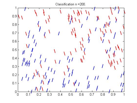
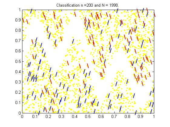
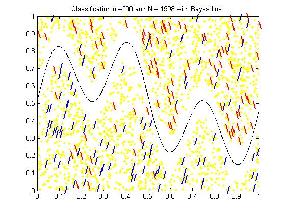
(a) (b) (c)

Figure 1: (a) The classified data; (b) Unlabeled data was added; (c) The boundary of the Bayes classifier was added

Semi-supervising classification is tempting. Consider Figure 1(a). The problem is finding the best classifier. Geometrically, we want to find the boundary between the area were most of the slashes are normal to area where there are mostly the back slashes. It is not an easy task. In Figure 1(b) we added unlabeled points. Now, it seems not that difficult to find the boundary. Since the figures were created by simulation, we can add the optimal boundary corresponding to the Bayes classifier. It is given in Figure 1(c), lying exactly where most readers thought it should be.

Here is an example where it is easy to see what is going on. Suppose $u_{1},u_{2},\dots,u_{K}$ are i.i.d. exponential with mean $\sigma$, $v_{1},v_{2},\dots,v_{K}$ are i.i.d. exponential with mean $\tau$. Let $a_{1}<b_{1}<a_{2}<b_{2}<\dots<a_{K}<b_{K}$, be such that $b_{i}-a_{i}={u_{i}}/(\sum u_{j}+\sum v_{j})$, and $a_{i+1}-b_{i}={v_{i}}/(\sum u_{j}+\sum v_{j})$. Now let the covariate $X_{1},X_{2},\dots,X_{N}$ be i.i.d. uniform on $\cup(a_{i},b_{i})$, the variables $p_{1},p_{1},\dots,p_{K}$ be i.i.d. $P(p_{i}=1)=P(p_{i}=0)=1/2$. Finally let the labels $Y_{1},\dots,Y_{n}$ be independent $P(Y_{i}=1|X)=\sum p_{j}\mbox{\Large$\mathbf{1}$}\Bigl{\{}X\in(a_{j},b_{i})\Bigr{\}}$. Consider now the asymptotic as $n\to\infty$, $n/N\to 0$, $n/K\to\gamma>0$, $\sigma/\tau\to\infty$, and $N\tau/\log(N)K\to\infty$.

The length of the support is 1, and there are $N$ observations uniformly distributed in it. Hence the largest spacing between observations belonging to same interval is $\mathcal{O}_{p}(\log(N)/N)$. The distance between adjacent intervals is approximately exponential, and hence the minimal distance between two adjacent intervals of the support is $\mathcal{O}_{p}(\tau/K)$. The ratio between these two is $\mathcal{O}_{p}\bigl{(}\log(N)K/N\tau\bigr{)}=\text{$\mathcal{O}$}_{p}(1)$. It follows, therefore, we can know where the spacing between any pair of adjacent unclassified observations is small and the two members belong to the same interval, and where the spacing is large and they belong to different intervals. Let $A_{j}$ and $B_{j}$ be the smallest and largest observed $X$ inside the interval $(a_{j},b_{j})$. Then $\sum|B_{j}-A_{n}|/\sum|b_{j}-a_{j}|\nearrow 1$. Hence with the unclassified data it is easy to reconstruct the interval structure. If $\gamma$ is large, an almost perfect classifier can be constructed: $\hat{Y}(x)=Y_{i(x)}$ where $i(x)$ is the first $i\in\{1,\dots,m_{n}\}$ such that $X_{i}$ and $x$ are in the same interval $[A_{j},B_{j}]$, and $1/2$ otherwise.

Let $(X_{(1)},Y_{(1)}),\dots,(X_{(n)},Y_{(n)})$ be the fully observed sample sorted such that $X_{(1)}<X_{(2)}<\dots<X_{(n)}$. Since $\sigma/\tau\to\infty$, most of the $(0,1)$ interval belongs to the support. Further, $\gamma$ is finite, hence we cannot know whether $X_{(i)}$ and $X_{(i+1)}$ belong to the same interval or not. If $Y_{(i)}\neq Y_{(i+1)}$, we know that $P(Y=1|x)$ is not constant on the interval $(X_{(i)},X_{(i+1)}))$, but not much more than that. The change point is almost uniformly distributed (it is if $\gamma$ is very small). If $Y_{(i)}=Y_{(i+1)}$, we know that it is quite likely that $P(Y=1|x)$ is not constant on the interval $(X_{(i)},X_{(i+1)}))$. In any case we cannot know perfectly well ${\rm E}\mathop{\!}\nolimits(Y|X)$ for a random $X$.

Clearly the classification error of an estimator based only on the unlabeled data is $1/2$—there is no way to know the values of the $p$’s given only the $X$’s. At the same time, any classifier based only on the label points is very weak and its classification error is close to the maximal $1/2$. However, the classification error of an classifier based on all the data is close to the minimal 0. The semi-supervising approach works because the way $P(Y=1|x)$ is constructed is strongly tied to the way the support of $X$ is constructed, and the statistician knows these ties pretty well.

Can we justify the transduction from the experiment with observations $X$ to the experiment with $(X,Y)$? From the distribution of $X$ to the conditional distribution of $Y$ given $X$? Certainly the answer is yes, when simulations are done. However, can we give a statistical (empirical) justification for that? The answer to this difficulty is usually, something like “see, it worked these many times, in this many best typical examples.” We suggest to take these answers with the same grain of salt, as answers who dismiss the need of confidence sets, or P-values (or their Bayesian counterparts), because “rejecting the null was typically successful”.

The transduction argument was successful in the above two simulations, because, the data was generated by a mechanism that tied together the value of the regression function, and the underlined covariate distributions. Note, however the following pseudo-theorem. Cf. [Bickel et al. (1998)] for a precise formulations and examples.

Meta-theorem 5.1

Suppose $(X,Y),(X_{1},Y_{1}),(X_{2},Y_{2})\dots,$ are i.i.d.. Suppose that $X\sim H$, $P(Y=1|X=x)=p_{\vartheta,\nu}(x)$, $(H,\nu)\in{\mathcal{H}}\times{\mathcal{N}}$. Then, the semiparametric bound for estimating $\vartheta=\vartheta(\nu)$ is the same whether the distribution $H$ of $X$ is known or unknown.

As we read the theorem it implies that there is no data dependent way to use the covariate distribution in a regular inference about the conditional distribution, at least locally and at the $\sqrt{n}$ rate. Any use of the covariate distribution, is based on a-priori assumed connection and cannot be quantified or justified empirically.

5.2 Preprocessing PCA

Preprocessing PCA is another version of the semi-supervised transduction, cf. [Jolliffe (1972)], [Jolliffe (1973)], and [Cook and Forzani (2008)]. Suppose that $X,X_{1},\dots,X_{N}$ are i.i.d., $X\in{\mathbb{R}}^{p}$. This sample is partially labeled with a $Y\in{\mathbb{R}}$, such that $(X,Y),(X_{1},Y_{1},),\dots,(X_{n},Y_{n})$ are i.i.d., and $(X,Y)$ follows a linear regression model. We consider the case where both $N\gg n$ and $p\gg n$. A common practice when there are too many variables, which is readily available in the semi-supervised state of mind, is reducing the number of variables using PCA (principal component analysis). This can be done using the all $X$ sample. After the PCA, we can regress $Y$ on the dominant $s$ main principal components, where $s\ll n$, and is chosen either $a-priori$, or in a data depended way (depending on $X_{1},\dots,X_{N}$).

The logic is irresistible. If $X=(X^{1},\dots,X^{p})^{\scriptstyle{\mathsf{T}}}$ and $\mathop{\rm cor}\nolimits(X^{1},X^{2})\approx 1$, we certainly can retain only the average $(X^{1}+X^{2})/2$, and ignore their difference. Thus reducing the number of variables by one. No much information is lost by this. However, this logic is transductive, and cannot be justified using the experimental $X$ data. It again based on some magic connection between the marginal distribution of $X$ and that of $Y$ given $X$. It appeals to some principal that says roughly that nothing is accidental. But this appeal to ‘justice’ is clearly fallible. It may that $Y$ is a function of the mismatch between $X^{1}$ and $X^{2}$, and not so much or their conjunction. For example, let $X^{1}$ be the optical power of the lenses a patient needs (in diopters), and $X^{2}$ those he actually uses. Luckily they are highly correlated, but presumably headache is caused by their small difference. For another example, tension within a couple maybe caused more by education difference than by education average.

5.3 Saving the transduction

We have a real problem if by semi-supervised learning we understand what [Gammerman et al. (1998)] refer to by: “This is the problem of transduction in the sense that we are interested in the classification of a particular example rather than in the general rule for classifying future examples.” However, with large data set a different point of view can be considered, and a more gentle interpretation is possible. Suppose we want to use the sample for prediction. The best predictor is nonparametric, and a-priori belongs to a very large set of potential predictors, too large to make useless any empirical risk minimizer which is based on the unlabeled data. However, one may use the unlabeled sample essentially for suggesting a small set of potential predictors. The final predictor to be chosen, is going to be selected from these potential predictors, and this selection is going to be done solely based on the labeled sample. This predictor can be compared to the predictor which is based solely on the unlabeled data, and the best of them can be used. In this way, if the unverifiable assumptions used for the semi-supervising reasoning are approximately valid, then they will be utilized, and if they yield a bad predictor, they will be discarded.

Let us repeat. The unlabeled data are used only in suggesting potential predictors, and not in the decision on the final predictor.

A similar argument can be used in the preprocessing PCA and the modified method is easily defensible. Co-linearity is not really a problem for prediction. With LASSO like techniques ([Tibshirani (1996)]), $p\gg n$ can be handled, as long as there is an approximation with only $p_{0}\ll n$ non-zero coefficients, cf. [Greenshtein and Ritov (2004)]. PCA preprocessing can be used to generate a new set of $q$, $q\ll p$ variables $Z^{1},\dots,Z^{q}$. One can regress $Y$ on $Z^{1},\dots,Z^{q}$, but for this one needs extra assumptions. One can regress $Y$ on $Z^{1},\dots,Z^{q},X^{1},\dots,X^{p}$ with very little extra assumptions. Then if the PCA step happened to be smart, it will be effective, and if information was lost in the PCA reduction, it will be regained.

6 Counterfactual causality

The counterfactual theory of causality.(cf. [Rubin (1974)], [Holland (1988)] and others)

• Each individual is characterized by two outcomes $(Y^{C},Y^{T})$. One under the control condition and one under the treatment condition.

• The “causal effect” is the difference between these two potential outcomes, i.e., $\delta=Y^{T}-Y^{C}$

• However,as mentioned, only one of these potential outcome is observed. The observation on subject $i$ is $(Y_{i},T_{i},X_{i})$, where

  $$Y_{i}=Y_{i}^{C}+T_{i}(Y_{i}^{T}-Y_{i}^{C}),\quad T\in\{0,1\}.$$

For example, each participant carries two outcomes (from birth?), the first would be expressed if he will smoke all his life, and the other if he wouldn’t. But the same subject may participate in another experiment, and therefore he has another couple of outcomes, where the first outcome will be measured if he would learn German in one type of program, and the other will be expressed if he would learn it by another.

The model can be summarized by $Y_{i}=Y_{i}^{C}+T_{i}\delta_{i},\quad T\in\{0,1\}$ When we are dealing with a well designed experiment with a random allocations of units, $T$ is independent of $(Y^{C},Y^{T})$, and the mean causal effect is easily estimated

$$\hat{}\delta =\frac{1}{n}_{1}\sum_{T_{i}=1}Y_{i}-\frac{1}{n}_{0}\sum_{T_{i}=0}Y_{i}$$

However, this metaphysics is used exactly when $T$ is not exogenous and in particular it is not independent of $(Y^{C},Y^{T})$. The different solutions of this basic “difficulty” are based on the assumption that $T$ is independent of $(Y^{C},Y^{T})$ conditional on a linear function of $X$.

Using a heavily loaded metaphysics in a naturally positivistic science as statistics is justified when either

1. It justifies in one sharp Ockhamian cut many many problems.

2. It really simplifies the analysis.

3. It unifies the terminology.

Neither of these conditions is satisfied here. First, is the ax sharp? Can the counterfactual theory of causality contribute anything a simple model cannot? What would be the case if the treatment is continuous? In reality, most “treatments” are continuous even if measured as either-or. People are not either passive smoker or passive non-smoker, study to the exam or come unprepared, either take the drug or not. In medical experiment, even if the control condition is objectively defined, the experiment condition is typically arbitrary chosen from a continuous set of doses, treatment durations, Should we use a continuity of counterfactuals? What happens if the “treatment” is multivariate? (Passive smoker in the work place, only once a hour, and once a week in pub…) A function of time? Simple it ain’t.

Does the counterfactual point of view simplifies the terminology? The natural terminology of the standard model $({\mathcal{Z}},{\mathcal{F}},\{P_{\vartheta}\})$ is that of conditional distribution. Hence we ask, does the model $Y=Y^{C}+T(Y^{T}-Y_{C})$ has any additive value over: The conditional distribution of $Y$ given $T=0$ has a different mean than its conditional distribution given $T=1$? We cannot dispense the conditional terminology altogether because we need to talk on the conditional distribution of $(T,Y^{C},Y^{T})$ given the covariate $X$. Hence, the counterfactual presentation does not simplifies the causality lexicon. It just adds new terms.

Some may say that it adds. It tells us about two different statistical models: $(Y,{\mathcal{F}},\{Q^{C}_{\vartheta}\}$ and $(Y,{\mathcal{F}},\{Q^{T}_{\vartheta}\}$. These models are useful if we want to consider the distribution of $Y$ if the unit is “enforced” to be in one of the two groups. After all this is what we really want. We want to know what the impact of a new no-smoking rule will have on life expectancy.

However, if we consider different statistical models, we could talk about a plentitude of them, not only on two. We can consider $(Y,{\mathcal{F}},\{Q^{t}_{\vartheta}\}$, $t\in\mathop{\rm supp}\nolimits T$, and certainly it may that $P_{\vartheta}^{t}(Y\in A)=P_{\vartheta}(Y\in A\;\big{|}\;T=t)$, and for this we do not need the counter factual terminology.

This last presentation is a transduction over the standard statistical model which talks only about ${P_{\vartheta}}$. We don’t have manipulated data in the sample, and hence any conclusion on manipulation is beyond the statistical reasoning. Typically it is just a wishful thinking. See for example [Bound et al. (1995)], for a causality argument based self-evident assumptions that happened not to be true. Wishes sometimes come true, but more often than not, they do not. Thus [Pearl (2009)] claims that “confounding bias cannot be detected or corrected by statistical methods alone”. More specifically. “This information must be provided by causal assumptions which identify relationships that remain invariant when external conditions change.” But, most often than not, this is petitio principii, or begging the question. One start with causal assumptions which are the empirical conclusion is disguise.

7 Conclusions

Transduction inference is unavoidable. One cannot avoid causality questions in the name of statistical integrity. One should realize that decision should be made, but one should recognize that they are not based on statistical safe ground. Certainly, quoting P-values and confidence intervals may be done only for the sake of style.

However, when we discussed the problems of prediction and semi-supervised learning we argued that when done carefully, almost transductive arguments can be used. In fact, one can use procedures that work nicely if his assumptions are valid, and do not fail him if they are not. If the time series is indeed stationary, then his predictors will be meaningful. If it is not, they would be trivial but right. The unlabeled data would be used to construct a better classifier if the right smoothness exists, otherwise it would not mislead the careful statistician.

References

- Altman and Bland (1998) Altman, D. G. and Bland, J. M. (1998). Generalisation and extrapolations. British Medical Journal, 317, 409–410.
- Amini and Gallinari (2005) Amini, R. and Gallinari, P. (2005). Semi-supervised learning with an imperfect supervisor. Knowledge and Information Systems, 8, 385–413.
- Belkin and Niyogi (2004) Belkin, M. and Niyogi, P. (2004). Semi-supervised learning on riemannian manifolds. Machine Learning, 56, 209–239.
- Berger (1993) Berger, J. O. (1993). Statistical Decision Theory And Bayesian Analysis (2nd ed.). Springer-Verlag, New York.
- Berger and Wolpert (1988) Berger, J. O. and Wolpert, R. L. (1988). The Likelihood Principle: A Review, Generalizations, and Statistical Implications (2nd ed.)., volume 6 of Lecture Notes—Monograph Series. IMS, Hayward, California.
- Bickel and Doksum (2000) Bickel, P. J. and Doksum, K. A. (2000). Mathematical Statistics, volume I. Prentice-Hall, Englewood Cliffs.
- Bickel et al. (1998) Bickel, P. J., Klaassen, C. A. J., Ritov, Y., and Wellner, J. A. (1998). Efficient and Adaptive Estimation for Semiparametric Models (Revised paperbound edition ed.). Springer, New York.
- Birnbaum (1962) Birnbaum, A. (1962). On the foundations of statistical inference. Journal of the American Statistical Association,, 57, 269–306.
- Bound et al. (1995) Bound, J., Jaeger, D. A., and Baker, R. M. (1995). Problems with instrumental variables estimation when the correlation between the instruments and the endogeneous explanatory variable is weak. Journal of the American Statistical Association, 90, 443–450.
- Cook and Forzani (2008) Cook, R. D. and Forzani, L. (2008). Principal fitted components for dimension reduction in regression. Statistical Science, 23, 485–501.
- Cox (1958) Cox, D. R. (1958). Some problems connected with statistical inference. The Annals of Mathematical Statistics, 29, 357–372.
- Dawid (1985) Dawid, A. P. (1985). Self-calibrating priors do not exist: Comment. Journal of the American Statistical Association, 80, 340–341.
- Foster and Vohra (1998) Foster, D. and Vohra, R. (1998). Asymptotic calibration. Biometrika, 85, 379–390.
- Foster (1999) Foster, D. P. (1999). A proof of calibration via blackwell s approachability theorem. Games and Economic Behavior, 29, 73–78.
- Fudenberg and Levine (1999) Fudenberg, D. and Levine, D. (1999). An easier way to calibrate. Games Econ. Behavior, 29, 131–137.
- Gammerman et al. (1998) Gammerman, A., Vovk, V., and Vapnik, V. (1998). Learning by transduction. In In Uncertainty in Artificial Intelligence, (pp. 148–155). Morgan Kaufmann.
- Greenshtein and Ritov (2004) Greenshtein, E. and Ritov, Y. (2004). Persistence in high-dimensional linear predictor selection and the virtue of overparametrization. Bernoulli, 10, 971–988.
- Heathcote (1995) Heathcote, J. A. (1995). Why do old men have big ears? British Medical Journal, 311, 1688.
- Holland (1988) Holland, P. (1988). Causal inference, path analysis, and recursive structural equations models. In C. Clogg (Ed.), Sociological Methodology (pp. 449–484). American Sociological Association, Washington, D. C.
- Joachims (1999) Joachims, T. (1999). Transductive inference for text classification using support vector machines. International Conference on Machine Learning (ICML), , 200–209.
- Jolliffe (1972) Jolliffe, I. I. (1972). Discarding variables in a principal component analysis. i: Artificial data. Journal of the Royal Statistical Society. Series C (Applied Statistics), 21, 160–173.
- Jolliffe (1973) Jolliffe, I. I. (1973). Discarding variables in a principal component analysis. ii: Real data. Journal of the Royal Statistical Society. Series C (Applied Statistics), 22, 21–31.
- Krugman (2009) Krugman, P. (2009). How did economists get it so wrong? New York Times, September 2.
- Le Cam (1986) Le Cam, L. (1986). Asymptotic Methods in Statistical Decision Theory. Springer-Verlag, New York.
- Oakes (1985) Oakes, D. (1985). Self-calibrating priors do not exist. Journal of the American Statistical Association, 80, 339.
- Pearl (2009) Pearl, J. (2009). Causal inference in statistics: An overview. Statistical Surveys, 3, 96–146.
- Rubin (1974) Rubin, D. (1974). Estimating causal effects of treatments in randomized and nonrandomized studies. Journal of Educational Psychology, 66, 688–701.
- Taleb (2007) Taleb, N. N. (2007). Black swans and the domain of statistics. The American Statistician, 61, 198–200.
- Tibshirani (1996) Tibshirani, R. (1996). Regression shrinkage and selection via the lasso. Journal of the Royal Statistical Society. Series B (Methodological), 58(1), 267–288.
- Tukey (1960) Tukey, J. W. (1960). Conclusions vs decisions. Technometrics, 2, 423–433.