Single-shot discrimination of quantum unitary processes

Abstract

We formulate minimum-error and unambiguous discrimination problems for quantum processes in the language of process positive operator valued measures (PPOVM). In this framework we present the known solution for minimum-error discrimination of unitary channels. We derive a “fidelity-like” lower bound on the failure probability of the unambiguous discrimination of arbitrary quantum processes. This bound is saturated (in a certain range of apriori probabilities) in the case of unambiguous discrimination of unitary channels. Surprisingly, the optimal solution for both tasks is based on the optimization of the same quantity called completely bounded process fidelity.

1 Introduction

Quantum Theory is intrinsically a statistical theory, which means that our predictions and conclusions are typically probabilistic (see for example [1, 2]). For instance, even having the best possible knowledge on the photon polarization and polarizer filter we cannot predict whether an individual photon will pass the polarizer, or not. For us, as observers, this event is random except for very specific cases. Consequently, the predictive abilities of Quantum Theory are necessarily formulated in the language of probabilities.

On the other hand, in experiments we do not meet directly with probabilities. If the statistical samples are sufficiently large to estimate the probabilities, our conclusions about the identities of quantum objects could have a deterministic flavor. The remaining uncertainties are related to potential incompleteness of the information contained in the measured probabilities. For example, a measurement of the $z$th component of the spin (by means of Stern-Gerlach experiment) does not tell us almost anything about the $x$th coordinate of the spin. However, after sufficiently many (infinitely) repetitions the $z$th component is determined perfectly without any uncertainty.

In this paper we shall focus on our ability to make conclusions based on measurements repeated at most finite (small) number of times. Our primary aim is to investigate the distinguishability of quantum channels having access only to limited number of tests. We shall be interested in two particular statistical tasks: minimum-error discrimination and unambiguous discrimination. Both of them were extensively studied in the case of states, however, the discrimination of quantum processes is still rather an unexplored research area. In particular, researchers investigated the minimum error distinguishability of unitary channels [3, 4]. Partial results were obtained also in the unambiguous discrimination [5, 6] and minimum-error discrimination of specific channels [8, 9, 7, 10, 11, 12].

This paper is structured as follows: In Sections I, II, and III we will introduce the necessary concepts and mathematical tools. The case of state discrimination is very briefly discussed in Section IV. The Section V presents the general framework for discrimination of channels and the discrimination of unitary channels is analyzed in details in Section VI.

2 Description of experiments

An experiment is a time ordered set of instructions that are divided into three procedures: i) preparation, ii) processing, iii) measurement. In quantum theory the quantum systems are associated with Hilbert spaces and the mathematical description of quantum objects (preparators, processes and measurements) is formulated in terms of specific operators and structures defined on the underlying Hilbert space ${\cal H}$.

The goal of preparations is to design a source of systems in particular quantum states, which are represented by density operators, i.e. positive linear operators of a unit trace. Let us denote by ${\cal S}({\cal H})$ the set of quantum states, i.e. ${\cal S}({\cal H})=\{\varrho:\varrho\geq O,{\rm tr}[\varrho]=1\}$. The events observed in the performed measurement are described by positive operators $O\leq E\leq I$ called also effects. Let us note that the positivity $A\geq O$ means that ${\langle\psi|}{A\psi\rangle}\geq 0$ for all $\psi\in{\cal H}$ and $A\geq B$ is equivalent to positivity of $A-B\geq O$. The probability to observe an effect $E$ providing that the measured state was $\varrho$ is given by the relation $p={\rm tr}[\varrho E]$. The whole measurement is described by a collection of effects $E_{1},\dots,E_{n}$ associated with $n$ mutually exclusive events forming a so-called positive operator valued measure (POVM), i.e. the normalization $\sum_{j}E_{j}=I$ holds. Thus, the observed probability distribution of outcomes $E_{1},\dots,E_{n}$ reads $p_{j}={\rm tr}[\varrho E_{j}]$.

In some cases it is convenient to include the processing part into either the preparation, or the measurement. However, in this paper the processes will be tested in experiments and therefore we shall consider them as devices independent of preparators and measurements. Mathematically, the processes are modeled as channels, i.e. completely positive trace-preserving linear maps defined on the set of trace-class operators ${\cal T}({\cal H})(\supset{\cal S}({\cal H}))$. In particular, a linear map ${\cal E}:{\cal T}({\cal H})\to{\cal T}({\cal H})$ is completely positive, if ${\cal I}\otimes{\cal E}[\Omega_{+}]\geq O$, where ${\cal I}$ denotes the identity map, $\Omega_{+}=\sum_{jk}|\varphi_{j}\otimes\varphi_{j}\rangle\langle\varphi_{k}\otimes\varphi_{k}|$ and $\varphi_{1},\dots,\varphi_{d}$ is an orthonormal basis of ${\cal H}$. It is trace-preserving if ${\rm tr}[{\cal E}[X]]={\rm tr}[X]$ for all trace-class operators $X\in{\cal T}({\cal H})$.

3 Classes of discrimination problems

In the discrimination problem the goal is to design an experiment in which an unknown quantum device (preparator, process, measurement) is used only once (or finite number of times) and from the observed outcome (sequence of outcomes) we want to determine which of $N$ expected elements “best” fits as the description of the unknown device. Let us denote by $X=\{x_{j}\}_{j\in J}$ the possible outcomes and let $\Omega=\{\omega_{1},\dots,\omega_{N}\}$ be the set of $N$ conclusions. The set $\Omega$ plays a dual role. It also represents the apriori information on the identity of the discriminated object in a sense that we know that the unknown device is one of the elements in $\Omega$. The conditional probability $p(x_{j}|\omega_{k})$ gives the probability to observe an outcome $x_{j}$ providing that the device is actually described by $\omega_{k}$. Defining the apriori distribution $\eta:\Omega\to[0,1]$ and using the Bayes rule we get the conditional probability

$$p(\omega_{k}|x_{j})=\frac{\eta_{k}p(x_{j}|\omega_{k})}{\sum_{l}\eta_{l}p(x_{j}|\omega_{l})}$$ (1)

evaluating the reliability of the conclusion $\omega_{k}$ providing that the outcome $x_{j}$ is observed. Let us note that $p_{j}=\sum_{l}\eta_{l}p(x_{j}|\omega_{l})$ is the total probability to observe the outcome $x_{j}$. If $p(\omega_{k}|x_{j})=1$ for some $\omega_{k}$, then the outcome $x_{j}$ uniquely determines conclusion $\omega_{k}$. We shall call such outcome and the related conclusion unambiguous. In all other cases, the conclusions are necessarily erroneous. In particular, $1-p(\omega_{k}|x_{j})$ is the related conditional error probability, when we choose the conclusion $\omega_{k}$ for the outcome $x_{j}$.

We can formulate many different discrimination problems. In what follows we shall consider two variations: minimum-error discrimination and unambiguous discrimination. In the so-called minimum-error discrimination [1], the goal is to minimize on average the errors we made in our conclusions. For simplicity, let us assume that the outcome $x_{j}$ leads to conclusion $\omega_{j}$. Then the average error reads

$$\overline{p}_{\rm error}=1-\sum_{j\in J}\eta_{j}p(x_{j}|\omega_{j})\,.$$ (2)

In the unambiguous discrimination problem the goal is either to achieve an unambiguous conclusion, or do not make any conclusion [13, 14, 15]. Therefore, the conclusions, if made, are error-free. However, not making any conclusion results in a nonvanishing failure probability, which on average reads

$$\overline{p}_{\rm fail}=\sum_{k\in J_{\rm inc}}\sum_{\omega_{j}\in\Omega}\eta_{j}p(x_{k}|\omega_{j})\,,$$ (3)

where $J_{\rm inc}$ denotes the set of indices associated with inconclusive outcomes. The aim is to minimize this quantity while satisfying the unambiguity of conclusions.

4 Discrimination of states

Discrimination problems for quantum states were investigated from many different perspectives, but in some versions the complete solutions are still not known. Let us briefly mention the basic results in the minimum-error discrimination of a preparator, which is known to produce one of the states $\varrho_{1}$, $\varrho_{2}$ with apriori probabilities $\eta_{1},\eta_{2}$, respectively. The statistics of the most general experiment we can perform might be formulated in the language of POVM, i.e. a pair of positive operators $E_{1},E_{2}$ such that $E_{1}+E_{2}=I$. That is, $\Omega=\{\varrho_{1},\varrho_{2}\}$ and $X=\{E_{1},E_{2}\}$, where outcome associated with $E_{j}$ is used to conclude $\varrho_{j}$. Since the probabilities are given by the formula $p(E_{j}|\varrho_{k})={\rm tr}[E_{j}\varrho_{k}]$ we get [1]

$$\overline{p}_{\rm error} = \min_{\rm POVM}\left(1-\eta_{1}{\rm tr}[E_{1}\varrho_{1}]-\eta_{2}{\rm tr}[E_{2}\varrho_{2}]\right)$$ (4)

$$= \frac{1}{2}\min_{\rm POVM}\left(1-{\rm tr}[(E_{1}-E_{2})(\eta_{1}\varrho_{1}-\eta_{2}\varrho_{2})]\right)$$

$$= \frac{1}{2}(1-{\rm tr}|\eta_{1}\varrho_{1}-\eta_{2}\varrho_{2}|)$$

$$= \frac{1}{2}(1-||\eta_{1}\varrho_{1}-\eta_{2}\varrho_{2}||_{\rm tr})\,,$$

where $||\cdot||_{\rm tr}={\rm tr}|\cdot|$ is the trace norm. The minimum is achieved for $E_{1}=\Pi_{+}$, where $\Pi_{+}$ is a projector onto the eigenvectors of the operator $\Delta=\eta_{1}\varrho_{1}-\eta_{2}\varrho_{2}$ associated with the positive eigenvalues.

Unlike the minimum-error discrimination the unambiguous one does not have a nontrivial solution for a general pair of states $\varrho_{1},\varrho_{2}$. There are cases in which the unambiguity requirements ${\rm tr}[E_{1}\varrho_{2}]={\rm tr}[E_{2}\varrho_{1}]=0$ cannot be satisfied. In the unambiguous discrimination we are looking for effects $E_{1},E_{2}$ such that $E_{1}+E_{2}\leq I$ and an effect $I-E_{1}-E_{2}$ represents the inconclusive outcome. In particular, the unambiguous discrimination is possible only if the supports of $\varrho_{1}$ and $\varrho_{2}$ do not coincide. Interestingly, if $\varrho_{1}$, $\varrho_{2}$ are apriori equally probable pure states $\psi,\varphi$, then $\overline{p}_{\rm fail}=|{\langle\psi|}{\varphi\rangle}|$ (see for example [13, 14, 15, 16, 17]). Although many interesting results have been discovered [17, 18, 19, 20, 21], we are lacking a closed formula for the optimal value of $\overline{p}_{\rm fail}$ in the general situation.

5 Discrimination of channels

In this section we shall formulate analogous discrimination problems for quantum processes, i.e. channels. A general experiment for probing them is described by the so-called process POVM in the same sense as POVM describes general experiment measuring the properties of quantum states. Process POVM provides a compact representation of the statistics generated by the most general experimental setup probing the properties of quantum channels.

The framework of PPOVM exploits a specific representation of channels defined via so-called Choi-Jamiolkowski isomorphism [22, 23, 24]. According to this theorem a channel on $d$ dimensional system can be represented by a positive operator acting on $d\times d$ system. In particular, a channel ${\cal E}$ is represented by an operator $\Omega_{\cal E}=({\cal I}\otimes{\cal E})[\Omega_{+}]$, where $\Omega_{+}=\sum_{j,k}|\varphi_{j}\otimes\varphi_{j}\rangle\langle\varphi_{k}\otimes\varphi_{k}|$. Let us note that $\Omega_{+}$ is not a projector, because it is not normalized and ${\rm tr}[\Omega_{+}]=d$. The operator $\frac{1}{d}\Omega_{+}$ is a one-dimensional projector onto the maximally entangled state $\psi_{+}=\frac{1}{\sqrt{d}}\sum_{j}\varphi_{j}\otimes\varphi_{j}\in{\cal H}\otimes{\cal H}$.

Process POVM is defined [25, 26] as a collection of positive operators (effects) $M_{1},\dots,M_{n}$ such that $\sum_{j}M_{j}=\xi^{T}\otimes I$ for some state $\xi\in{\cal S}({\cal H})$. An event that can be observed in the experiment consists of a preparation of the test state $\varrho$ and an observation of the effect $E_{j}$ in the measurement $E$ of the output state. Let us note that in the experiment we are allowed to use an ancilla of arbitrary size, i.e. $\varrho$ and $E_{j}$ are operators defined on $d_{\rm anc}\times d$-dimensional Hilbert space. The conditioned probability to observe an event consisting of the state preparation $\varrho$ and the observation of an effect $E_{j}$ providing that channel ${\cal E}$ is tested equals

$$p(\varrho,E_{j}|{\cal E})={\rm tr}[E_{j}({\cal I}\otimes{\cal E})[\varrho]]\,.$$ (5)

Using the Choi-Jamiokowski relation $\varrho=({\cal R}_{\varrho}\otimes{\cal I})[\Omega_{+}]$, where ${\cal R}_{\varrho}:{\cal T}({\cal H})\to{\cal T}({\cal H}_{\rm anc})$ is a completely positive map, and the duality relation ${\rm tr}[Y{\cal F}[X]]={\rm tr}[{\cal F}^{*}[Y]X]$ determining the dual channel ${\cal F}^{*}$ we can write

$$p(\varrho,E_{j}|{\cal E}) = {\rm tr}[({\cal R}_{\varrho}^{*}\otimes{\cal I})[E_{j}]({\cal I}\otimes{\cal E})[\Omega_{+}]]$$ (6)

$$= {\rm tr}[M_{j}\Omega_{\cal E}]\,,$$

where $M_{j}$ is an element of PPOVM. By definition $M_{j}$ is positive and $\sum_{j}M_{j}=({\cal R}^{*}_{\varrho}\otimes{\cal I})[I]=\xi^{T}\otimes I$, where $\xi={\rm tr}_{\rm anc}[\varrho]$. Thus, any experiment in which the channel is used once can be formalized as a PPOVM and the converse also holds [25], i.e. any PPOVM can be experimentally implemented.

5.1 Minimum-error discrimination

The framework of PPOVM is very useful for the formulation of the discrimination problems, because we do not have to consider all the details related to preparation of the test states and measurements. Let us formulate the minimum-error discrimination problem for a pair of channels ${\cal E}_{1},{\cal E}_{2}$ represented by operators $\Omega_{1},\Omega_{2}$. Analogously as in the case of states the aim is to design a PPOVM (given by $M_{1},M_{2}$) minimizing the error probability

$$\overline{p}_{\rm error}=\frac{1}{2}\min_{\rm PPOVM}\left(1-{\rm tr}[(M_{1}-M_{2})(\eta_{1}\Omega_{1}-\eta_{2}\Omega_{2})]\right)\,,$$

where $M_{1}+M_{2}=\xi^{T}\otimes I$ for some state $\xi$. Although this formula is similar to the one for the state discrimination, the optimization is due to the freedom in the normalization of the PPOVM more complex and not yet sufficiently understood. In fact, $\xi^{T}$ cannot be $I$, because ${\rm tr}[\xi^{T}]=1$. Therefore, the optimization for channels does not reduce to an optimization for states. For instance, pure states can be perfectly distinguished only if they are orthogonal, however, for unitary channels the orthogonality (with respect to the Hilbert-Schmidt scalar product) is only a sufficient condition [3, 4].

For every PPOVM there exists a pure test state realization, i.e. $M_{j}={\cal R}_{\psi}^{*}\otimes{\cal I}[F_{j}]$ for some pure test state represented by a unit vector $\psi\in{\cal H}\otimes{\cal H}$ and $\{F_{1},F_{2}\}$ is a POVM defined in ${\cal H}\otimes{\cal H}$ system. Expressing PPOVM elements in this way we obtain a well-known formula for the minimum error probability (see for example [27, 9])

$$\overline{p}_{\rm error} = \frac{1}{2}-\frac{1}{2}\sup_{\psi,F_{1},F_{2}}{\rm tr}[(F_{1}-F_{2})({\cal I}\otimes(\eta_{1}{\cal E}_{1}-\eta_{2}{\cal E}_{2}))[P_{\psi}]]$$ (7)

$$= \frac{1}{2}-\frac{1}{2}\sup_{\psi}{\rm tr}|({\cal I}\otimes(\eta_{1}{\cal E}_{1}-\eta_{2}{\cal E}_{2}))[P_{\psi}]|$$

$$= \frac{1}{2}(1-||\eta_{1}{\cal E}_{1}-\eta_{2}{\cal E}_{2}||_{\rm cb})$$

where $||\cdot||_{\rm cb}$ is the so-called norm of complete boundedness [28] and $P_{\psi}=|\psi\rangle\langle\psi|$.

A simple upper bound on this probability is given by an experiment in which the maximally entangled state $\psi_{+}$ is used as the test state, i.e. $M_{j}=\frac{1}{d}F_{j}$, where $F_{j}$ are effects forming the performed POVM, hence $M_{1}+M_{2}=\frac{1}{d}I\otimes I$. The bound reads

$$\overline{p}_{\rm error}\leq\frac{1}{2}(1-\frac{1}{d}{\rm tr}|\eta_{1}\Omega_{1}-\eta_{2}\Omega_{2}|)\,.$$ (8)

Another interesting bound comes from the experiments in which no ancilla is used, i.e. $M_{j}=|\psi\rangle\langle\psi|^{T}\otimes F_{j}$, where $F_{j}$ is the POVM measurement of the output state. In such case

$$\overline{p}_{\rm error}\leq\frac{1}{2}(1-\max_{\psi\in{\cal H}}||(\eta_{1}{\cal E}_{1}-\eta_{2}{\cal E}_{2})[P_{\psi}]||_{\rm tr})\,.$$ (9)

5.2 Unambiguous discrimination

In the case of the unambiguous discrimination the problem is formulated by means of the following equations

$${\rm tr}[M_{1}\Omega_{2}]={\rm tr}[M_{2}\Omega_{1}]=0$$ (10)

$$\overline{p}_{\rm failure}=\min_{M_{0}}{\rm tr}[M_{0}(\eta_{1}\Omega_{1}+\eta_{2}\Omega_{2})]$$ (11)

under the PPOVM constraint

$$M_{0}+M_{1}+M_{2}=\xi^{T}\otimes I$$ (12)

for some state $\xi\in{\cal S}({\cal H})$.

In the following proposition we shall formulate a lower bound on the probability of failure, which is analogous to the bound known for the unambiguous discrimination of two mixed states (see for instance [19]).

Proposition 5.1.

Let ${\cal E}_{1},{\cal E}_{2}$ be channels and $\eta_{1},\eta_{2}$ be their apriori probabilities. Then

$$\overline{p}_{\rm failure}\geq 2\sqrt{\eta_{1}\eta_{2}}\min_{\xi\in{\cal S}({\cal H})}{\rm tr}|\sqrt{\Omega_{1}}(\xi^{T}\otimes I)\sqrt{\Omega_{2}}|\,,$$ (13)

where $\Omega_{j}=({\cal I}\otimes{\cal E}_{j})[\Omega_{+}]$.

Proof 5.2.

Since for all numbers $a^{2}+b^{2}\geq 2ab$ and setting $a=\eta_{1}{\rm tr}[M_{0}\Omega_{1}]$, $b=\eta_{2}{\rm tr}[M_{0}\Omega_{2}]$ we get

$$\overline{p}^{2}_{\rm failure}\geq 4\eta_{1}\eta_{2}{\rm tr}[M_{0}\Omega_{1}]{\rm tr}[M_{0}\Omega_{2}]\,.$$ (14)

Using the Cauchy-Schwartz inequality we obtain

$${\rm tr}[M_{0}\Omega_{1}]{\rm tr}[M_{0}\Omega_{2}]=$$

$$\quad={\rm tr}[U\Omega_{1}^{\frac{1}{2}}M_{0}^{\frac{1}{2}}M_{0}^{\frac{1}{2}}\Omega_{1}^{\frac{1}{2}}U^{\dagger}]{\rm tr}[\Omega_{2}^{\frac{1}{2}}M_{0}^{\frac{1}{2}}M_{0}^{\frac{1}{2}}\Omega_{2}^{\frac{1}{2}}]$$

$$\quad\geq({\rm tr}[U\sqrt{\Omega_{1}}M_{0}\sqrt{\Omega_{2}}])^{2}\,.$$

By definition $M_{0}=\xi^{T}\otimes I-M_{1}-M_{2}$. Since the no-error conditions $\Omega_{1}M_{2}=M_{1}\Omega_{2}=O$ hold, it follows that $\sqrt{\Omega_{1}}M_{0}\sqrt{\Omega_{2}}=\sqrt{\Omega_{1}}(\xi^{T}\otimes I)\sqrt{\Omega_{2}}$, thus,

$$\overline{p}_{\rm failure}\geq 2\sqrt{\eta_{1}\eta_{2}}|{\rm tr}[U\sqrt{\Omega_{1}}(\xi^{T}\otimes I)\sqrt{\Omega_{2}}]|\,.$$ (15)

Using the identity $\sup_{U}|{\rm tr}[XU]|={\rm tr}|X|$ holding for all operators $X$ the inequality reads

$$\overline{p}_{\rm failure}\geq 2\sqrt{\eta_{1}\eta_{2}}{\rm tr}|\sqrt{\Omega_{1}}(\xi^{T}\otimes I)\sqrt{\Omega_{2}}|\,,$$ (16)

which proves the lemma after the optimalization over the PPOVM normalization is taken into account.

The function $D(\Omega_{1},\Omega_{2})=\min_{\xi}{\rm tr}|\sqrt{\Omega_{1}}(\xi\otimes I)\sqrt{\Omega_{2}}|$ we shall call completely bounded process fidelity in analogy with the completely bounded norm $||\cdot||_{\rm cb}$. Let us note that both $\xi$ and $\xi^{T}$ are states, thus the transposition is irrelevant in the formula for $D$. This quantity was introduced in Ref.[29] under the name minimax fidelity as the abstract channel analogy of the state fidelity. Since [29]

$$1-\frac{1}{2}||{\cal E}_{1}-{\cal E}_{2}||_{\rm cb}\leq D(\Omega_{1},\Omega_{2})\leq\sqrt{1-\frac{1}{4}||{\cal E}_{1}-{\cal E}_{2}||_{\rm cb}^{2}}\,,$$ (17)

we get $2\overline{p}_{\rm error}\leq D(\Omega_{1},\Omega_{2})$ for $\eta_{1}=\eta_{2}=1/2$. Consequently, if the identity $D({\cal E}_{1},{\cal E}_{2})=\min_{\xi}{\rm tr}|\sqrt{\Omega_{1}}(\xi\otimes I)\sqrt{\Omega_{2}}|=0$ holds, the channels ${\cal E}_{1},{\cal E}_{2}$ can be perfectly discriminated. Equivalently, the condition

$$\Omega_{1}(\xi\otimes I)\Omega_{2}=O$$ (18)

(holding for some density operator $\xi$) implies that the channels represented by $\Omega_{1},\Omega_{2}$ are perfectly distinguishable, and vice versa [30].

6 Unitary channels

In this section we shall focus on the discrimination of a pair of unitary channels. The minimum-error approach was investigated in [3, 4] and the unambiguous approach was adopted by Chefles et al. in [5]. Unitary channels are associated with Choi-Jamiokowski operators proportional to one-dimensional projectors. In particular, ${\cal E}_{U}=U\cdot U^{\dagger}$ is represented by $\Omega_{U}=d|\psi_{U}\rangle\langle\psi_{U}|$, where $\psi_{U}=(I\otimes U)\psi_{+}$. Given a pair of unitary channels $U,V$, then the joint support of $\Omega_{U},\Omega_{V}$ specifies a two-dimensional subspace ${\cal Q}$ of ${\cal H}\otimes{\cal H}$, which is relevant for both discrimination problems.

6.1 Minimum-error approach

Evaluation of the cb-norm $||\eta_{U}{\cal E}_{U}-\eta_{V}{\cal E}_{V}||_{\rm cb}$ will give us the solution for the minimum-error discrimination. Each unit vector $\psi$ can be expressed as $\psi=(A\otimes I)\psi_{+}$, thus, $P_{\psi}=({\cal R}_{\psi}\otimes{\cal I})[\Omega_{+}]=\frac{1}{d}(A\otimes I)\Omega_{+}(A^{\dagger}\otimes I)$. Moreover, since the following identity holds for any pair of vectors $\psi,\varphi$ and apriori probabilities $\eta_{\psi},\eta_{\varphi}$

$${\rm tr}|\eta_{\psi}|\psi\rangle\langle\psi|-\eta_{\varphi}|\varphi\rangle\langle\varphi||=\sqrt{1-4\eta_{\psi}\eta_{\varphi}|{\langle\psi|}{\varphi\rangle}|^{2}}$$

we get [4] the formula

$$\overline{p}_{\rm error} = \frac{1}{2}(1-||\eta_{U}{\cal E}_{U}-\eta_{V}{\cal E}_{V}||_{\rm cb})$$ (19)

$$= \frac{1}{2}(1-\sqrt{1-4\eta_{U}\eta_{V}D^{2}})\,,$$

where

$$D = \min_{A:{\rm tr}[A^{\dagger}A]=d}|{\langle(A\otimes U)\psi_{+}|}{(A\otimes V)\psi_{+}\rangle}|$$ (20)

$$= \frac{1}{d}\min_{A}|{\rm tr}[(A^{\dagger}A)^{T}U^{\dagger}V]|$$

$$= \min_{\xi\in{\cal S}({\cal H})}|{\rm tr}[\xi U^{\dagger}V]|\,.$$

We used the identities $(A\otimes I)\psi_{+}=(I\otimes A^{T})\psi_{+}$ and $dA^{\dagger}A={\rm tr}_{\rm anc}|(A\otimes I)\psi_{+}\rangle\langle(A\otimes I)\psi_{+}|=\xi^{T}$, where $\xi$ denotes the reduced state of the subsystem entering the tested quantum channel.

6.2 Unambiguous approach

Since supports of $\Omega_{U}$ and $\Omega_{V}$ are different, two unitaries can be always unambiguously distinguished. Let us denote by $Q$ a projector onto the linear subspace ${\cal Q}$ spanned by vectors $\psi_{U},\psi_{V}$. The unambiguous no-error conditions require that on the relevant subspace ${\cal Q}$ the operators $M_{U},M_{V}$ are rank-one and take the form

$$M_{U}^{\cal Q} = c_{U}(Q-|\psi_{V}\rangle\langle\psi_{V}|)\,,$$ (21)

$$M_{V}^{\cal Q} = c_{V}(Q-|\psi_{U}\rangle\langle\psi_{U}|)\,.$$ (22)

In addition, $M_{U}+M_{V}\leq\xi^{T}\otimes I$ for some state $\xi$. The success probability $\overline{p}_{\rm success}=1-\overline{p}_{\rm failure}$ reads

$$\overline{p}_{\rm success}=\max_{\rm PPOVM}\left(\eta_{U}{\rm tr}[M_{U}\Omega_{U}]+\eta_{V}{\rm tr}[M_{V}\Omega_{V}]\right)$$

$$\quad=\max_{\rm PPOVM}\left(\eta_{U}{\rm tr}[M_{U}^{\cal Q}\Omega_{U}]+\eta_{V}{\rm tr}[M_{V}^{\cal Q}\Omega_{V}]\right)$$

$$\quad=\max_{\varphi}\max_{\rm POVM}\left(\langle\varphi_{U}|\eta_{U}F_{U}|\varphi_{U}\rangle+\langle\varphi_{V}|\eta_{V}F_{V}|\varphi_{V}\rangle\right)$$

As previously, we used the fact that PPOVM can be always implemented using a pure test state. This test state is associated with a suitable vector $\varphi=(A\otimes I)\psi_{+}$ leading to $M_{U}=(A^{\dagger}\otimes I)F_{U}(A\otimes I)$, $M_{V}=(A^{\dagger}\otimes I)F_{V}(A\otimes I)$, where effects $F_{U},F_{V}$ represent the conclusive outcomes of the performed POVM, i.e. $F_{U}+F_{V}\leq I\otimes I$. We used the notation $\varphi_{U}=(I\otimes U)\varphi$ and $\varphi_{V}=(I\otimes V)\varphi$.

For a fixed test state $|\varphi\rangle\langle\varphi|$ the POVM maximizing the expression $\langle\varphi_{U}|\eta_{U}F_{U}|\varphi_{U}\rangle+\langle\varphi_{V}|\eta_{V}F_{V}|\varphi_{V}\rangle$ is known from the analogous problem of unambiguous pure state discrimination [16, 17]. Without loss of generality we can assume that $\eta_{U}\geq\eta_{V}$. In such case the optimal POVM consists of effects

$$F_{U}=\min\left\{\frac{1-\sqrt{\frac{\eta_{V}}{\eta_{U}}}|{\langle\varphi_{U}|}{\varphi_{V}\rangle}|}{1-|{\langle\varphi_{U}|}{\varphi_{V}\rangle}|^{2}},1\right\}(Q_{\varphi}-|\varphi_{V}\rangle\langle\varphi_{V}|)\,,$$

$$F_{V}=\max\left\{\frac{1-\sqrt{\frac{\eta_{U}}{\eta_{V}}}|{\langle\varphi_{U}|}{\varphi_{V}\rangle}|}{1-|{\langle\varphi_{U}|}{\varphi_{V}\rangle}|^{2}},0\right\}(Q_{\varphi}-|\varphi_{U}\rangle\langle\varphi_{U}|)\,,$$

where $Q_{\varphi}$ is a projector onto the subspace spanned by vectors $\varphi_{U},\varphi_{V}$. The failure probability $\overline{p}_{\rm failure}=1-\overline{p}_{\rm success}$ reads

$$\overline{p}_{\rm failure}=\left\{\begin{array}[]{ll}2\sqrt{\eta_{U}\eta_{V}}D&{\rm if}\ D\leq\sqrt{\frac{\eta_{V}}{\eta_{U}}}\leq 1\\ \eta_{V}+\eta_{U}D^{2}&{\rm if}\ D\geq\sqrt{\frac{\eta_{V}}{\eta_{U}}}\leq 1\end{array}\right.\,,$$

where we used the definition $D=\min_{\varphi}|{\langle\varphi_{U}|}{\varphi_{V}\rangle}|=\min_{\xi\in{\cal S}({\cal H})}|{\rm tr}[\xi^{T}U^{\dagger}V]|$ coinciding with Eq.(20).

Let us note that the considered unambiguous discrimination of unitary channels saturates the bound specified in Proposition 5.1 for values $D\leq\sqrt{\frac{\eta_{V}}{\eta_{U}}}$. Indeed, since ${\rm tr}|X|={\rm tr}\sqrt{X^{\dagger}X}$ and $\sqrt{\Omega_{U}}=\sqrt{d}|\psi_{U}\rangle\langle\psi_{U}|$, $\sqrt{\Omega_{V}}=\sqrt{d}|\psi_{V}\rangle\langle\psi_{V}|$ the bound gives

$$\overline{p}_{\rm failure} \geq 2\sqrt{\eta_{U}\eta_{V}}\min_{\xi}{\rm tr}|\sqrt{\Omega_{U}}(\xi^{T}\otimes I)\sqrt{\Omega_{V}}|$$

$$= 2d\sqrt{\eta_{U}\eta_{V}}\min_{\xi}|{\langle\psi_{U}|}{(\xi^{T}\otimes I)\psi_{V}\rangle}|{\rm tr}[|\psi_{U}\rangle\langle\psi_{U}|]$$

$$= 2\sqrt{\eta_{U}\eta_{V}}\min_{\xi}|{\rm tr}[\xi^{T}U^{\dagger}V]|$$

$$= 2\sqrt{\eta_{U}\eta_{V}}D\,,$$

where we used the identity ${\langle\psi_{U}|}{(\xi^{T}\otimes I)\psi_{V}\rangle}=\frac{1}{d}{\rm tr}[\xi^{T}U^{\dagger}V]$. If $D\geq\sqrt{\frac{\eta_{V}}{\eta_{U}}}$, then $\overline{p}_{\rm failure}=\eta_{V}+\eta_{U}D^{2}>2\sqrt{\eta_{U}\eta_{V}}D$, because $(\sqrt{\eta_{V}}-D\sqrt{\eta_{U}})^{2}\geq 0$. We see that this bound is not achievable in general. In fact, the existence of the PPOVM giving the bound is not guaranteed in its derivation. The particular process discrimination problem could pose additional constraints on the possible choices of the normalization $\xi^{T}\otimes I$, which makes the value of $D$, hence also the bound, different.

6.3 Evaluation of $D$

It follows that the optimal solutions of both discrimination problems for unitary channels is based on minimalization of the same quantity $D$, which is called completely bounded process fidelity. This quantity was also analyzed in the study of perfect discrimination of unitary channels [3, 4] and we will repeat the analysis. Let us denote by $\{\phi_{k}\}$ the eigenvectors of $U^{\dagger}V$ associated with eigenvalues $e^{i\theta_{k}}$. Then

$$D=\min_{\xi\in{\cal S}({\cal H})}|\sum_{k}e^{i\theta_{k}}\langle\phi_{k}|\xi|\phi_{k}\rangle|\,.$$ (23)

The number on the right hand side is a convex combination of complex square roots of unity. Thus, it can be visualized as an element of the convex hull of points (eigenvalues of $U^{\dagger}V$) on the unit circle of the complex plane. Our aim is to find the complex number within this convex hull which is closest to zero. In particular, if 0 is not contained in the convex hull, then

$$D=\frac{1}{2}\min_{k,l}|e^{i\theta_{k}}+e^{i\theta_{l}}|\,,$$ (24)

which means a suitable test state has only two nonvanishing entries (equal to 1/2) on the diagonal of its reduced state $\xi$ (see Figure 1).

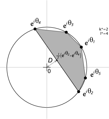
Figure 1: Illustration of the completely bounded process fidelity $D$ for unitary channels in the case, when the convex hull of eigenvalues of $U^{\dagger}V$ does not contain 0.

Since for two-dimensional Hilbert space the unitary operators have only two eigenvalues, the minimalization is trivial [3] and reads

$$D=\frac{1}{2}|e^{\i\theta_{1}}+e^{i\theta_{2}}|=\frac{1}{2}|{\rm tr}[U^{\dagger}V]|\,.$$ (25)

Hence in this case the orthogonality in the Hilbert-Schmidt sense is necessary and sufficient for perfect discrimination of ${\cal E}_{U}$ and ${\cal E}_{V}$. Moreover, the maximally entangled state (for which $\xi=\frac{1}{2}I$) is the universal test state optimizing the minimum-error and unambiguous discrimination. Of course, the measurements depend on the particular task and the unitaries. However, these properties do not hold in the higher dimensions. For example, CNOT and SWAP gate can be perfectly discriminated even without being orthogonal and the maximally entangled test state is not very usable.

The minimum in the definition of $D$ (see Eq.(23)) depends only on the diagonal entries of $\xi$, thus we can always choose optimal $\xi$ to be a pure state. That is, no ancilla is needed in order to implement an optimal discrimination experiment. Formally, the optimal test state can be chosen to be factorized $\psi=\psi_{A}\otimes\psi_{S}$, where $\psi_{A}$ is arbitrary and $\psi_{S}$ is the pure test state with suitable diagonal elements $|{\langle\phi_{k}|}{\psi_{S}\rangle}|^{2}$. Let us assume that $k^{*},l^{*}$ are indexes of the eigenvalues optimizing the average error probability. Then, $\psi_{S}=\frac{1}{\sqrt{2}}(\varphi_{k^{*}}+\varphi_{l^{*}})$ is the vector associated with an optimal test state. For any apriori probabilities $\eta_{U},\eta_{V}$ this single test state is optimal for both minimum error and unambiguous discrimination. The optimal experiments for these tasks differ in the used measurements, which depends also on the apriori probabilities.

7 Conclusion

The discrimination of quantum devices provides us with a clear operational definition of their closeness. Apart from this purely mathematical motivation, the discrimination problems naturally appear in various communication and computation problems. In this paper we formulated the minimum-error and unambiguous single-shot discrimination among two quantum processes using the language of PPOVM. In this framework we can clearly see the differences between the discrimination tasks for states and for processes. Many of the results derived for states can be translated to channels, however, there are also some significant differences. As for example, the perfect distinguishability of pure states and unitary channels [3, 4]. For the minimum-error approach the trace norm is replaces by completely bounded norm, which is not that easy to evaluate in general [31, 32]. We derived a simple lower bound on the probability of failure for unambiguous discrimination of quantum channels

$$\overline{p}_{\rm failure}\geq 2\sqrt{\eta_{U}\eta_{V}}D(\Omega_{1},\Omega_{2})\,.$$ (26)

This bound suggests a state fidelity equivalent for channels called completely bounded process fidelity

$$D(\Omega_{1},\Omega_{2})=\min_{\xi}{\rm tr}|\sqrt{\Omega_{1}}(\xi\otimes I)\sqrt{\Omega_{2}}|\,,$$ (27)

where $\Omega_{j}=({\cal I}\otimes{\cal E}_{j})[\Omega_{+}]$ are the Choi-Jamiolkowski operators associated with the channels ${\cal E}_{j}$. Let us remind that in the case of minimum-error discrimination the optimal value of error probability equals

$$\overline{p}_{\rm error}=\frac{1}{2}(1-||\eta_{1}{\cal E}_{1}-\eta_{2}{\cal E}_{2}||_{\rm cb})\,.$$ (28)

For unitary channels we have shown that both discrimination problems reduce to the optimization of the same quantity. Moreover, in this case the lower bound on the probability of failure is saturated. In particular, for equal apriori probabilities $\eta_{U}=\eta_{V}=1/2$ we have

$$\overline{p}_{\rm error} = \frac{1}{2}(1-\sqrt{1-D^{2}})\,,$$ (29)

$$\overline{p}_{\rm failure} = D\,,$$ (30)

where

$$D=D({\cal E}_{U},{\cal E}_{V})=\min_{\xi}{\rm tr}|\xi U^{\dagger}V|\,.$$ (31)

Interestingly, no ancilla is required and the same pure test states optimizes both probabilities simultaneously. The difference is in the measurement performed on the channel output.

A lot of work remains to be done in the area of process discrimination and identification. We believe that a better understanding to distinguishability of general quantum processes is related to the development of the theory of PPOVM, which currently serves as a useful tool for numerical optimization. However, to get a deeper understanding of discrimination problems it seems crucial to be able to characterize those PPOVMs that are compatible with the given constraints.

Acknowledgments

We acknowledge financial support via the European Union projects QAP 2004-IST-FETPI-15848, HIP FP7-ICT-2007-C-221889, and via the projects APVV-0673-07 QIAM, VEGA-2/0092/09, OP CE QUTE ITMS NFP 262401022, and CE-SAS QUTE.

References

• [1] C.W. Helstrom, Quantum Detection and Estimation Theory (Academic Press, New York, 1976).
• [2] A. Peres, Quantum Theory: Concepts and Methods (Kluwer 1996)
• [3] A. Acin, Phys. Rev. Lett 87, 177901 (2001).
• [4] G.M. D’Ariano, P.L. Presti, M.G.A. Paris, Phys. Rev. Lett. 87, 270404 (2001).
• [5] A. Chefles, A. Kitagawa, M. Takeoka, M. Sasaki, J. Twamley, J. Phys. A 40 10183-10213 (2007) [quant-ph/0702245].
• [6] G. Wang, M. Ying, Phys. Rev. A 73, 042301 (2006) [quant-ph/0512142].
• [7] J. Watrous, Quantum Information and Computation 8, 819-833 (2008) [arXiv:0710.0902]
• [8] M.F. Sacchi, J. Opt. B 7, S333 (2005).
• [9] M.F. Sacchi, Phys. Rev. A 71, 062340 (2005).
• [10] M.F. Sacchi, Phys. Rev. A 72, 014305 (2005).
• [11] L. Li, D. Qiu, [arXiv:0705.2549]
• [12] M. Piani, J. Watrous, [arXiv:0901.2118]
• [13] I.D. Ivanovic, Phys. Lett. A 123, 257 (1987).
• [14] D. Dieks, Phys. Lett. A 126, 303 (1988).
• [15] A. Peres, Phys. Lett. A 128, 19 (1988).
• [16] G. Jaeger and A. Shimony, Phys. Lett. A 197, 83 (1995).
• [17] T. Rudolph, R.W. Spekkens, P.S. Turner, Phys.Rev.A 68, 010301(R) (2003).
• [18] P. Raynal, N. Lütkenhaus, S.J. van Enk, Phys.Rev. A 68, 022308 (2003)
• [19] Y. Feng, R. Duan, M. Ying, Phys. Rev. A 70, 012308 (2004), [arXiv:quant-ph/0403147]
• [20] U. Herzog, J.A. Bergou, Phys. Rev. A 71, 050301(R) (2005)
• [21] M. Kleinmann, H. Kampermann and D. Bruss, arXiv:0807.3923 (2008)
• [22] J. de Pillis, Pacific Journal of Mathematics 23, 129-137 (1967)
• [23] A. Jamiolkowski, Rep. Math. Phys. 3, 275 (1972).
• [24] M. Choi, Linear Algebra and its Applications, 10 (3): 285-290, (1975).
• [25] M. Ziman, Phys. Rev. A 77, 062112 (2008) [arXiv:0802.3862]
• [26] G. Chiribella, G.M. D’Ariano, and P. Perinotti, Europhysics Letters 83, 30004 (2008) [arXiv:0804.0180]
• [27] M. Raginsky, Phys. Rev. A 65, 032306 (2002) [quant-ph/0105141]
• [28] V.I. Paulsen, Completely bounded maps and operator algebras, Pitman Research Notes in Math. 146. (Longman Scietific and Technical, Harlow, 1996)
• [29] V.P. Belavkin, G.M. D’Ariano, M. Raginsky, J. Math. Phys. 46 062106 (2005), [quant-ph/0408159]
• [30] G. Chiribella, G.M. D’Ariano, P. Perinotti, Phys. Rev. Lett. 101, 180501 (2008), [arXiv:0803.3237]
• [31] B. Rosgen, J. Watrous, In Proceedings of 20th Annual Conference on Computational Complexity, 344-354 (2005)
• [32] J. Watrous, [arXiv:0901.4709]