Neutrino Masses and a TeV Scale Seesaw Mechanism

Abstract

A simple extension of the Standard Model providing TeV scale seesaw mechanism is presented. Beside the Standard Model particles and right-handed Majorana neutrinos, the model contains a singly charged scalar, an extra Higgs doublet and three vector like singly charged fermions. In our model, Dirac neutrino mass matrix raises only at the loop level. Small but non-zero Majorana neutrino masses come from integrating out heavy Majorana neutrinos, which can be at the TeV scale. The phenomenologies of the model are investigated, including scalar mass spectrum, neutrino masses and mixings, lepton flavor violations, heavy neutrino magnetic moments as well as possible collider signatures of the model at the LHC.

I Introduction

The observation of neutrino oscillations sno ; abcc ; kamland ; k2k has revealed that neutrinos have small but non-zero masses and lepton flavors are mixed, which can not be accommodated in the Standard Model (SM) without introducing extra ingredients. As such, neutrino physics offer an exciting window into new physics beyond the SM. Perhaps the most attractive approach towards understanding the origin of small neutrino masses is using the dimension-five weinberg operator weinberg :

$${1\over 4}\kappa_{gf}\overline{\ell_{Lc}^{C}}^{g}\varepsilon_{cd}\phi_{d}\ell_{Lb}^{f}\varepsilon_{ba}\phi_{a}+{\rm h.c.}\;,$$ (1)

which comes from integrating out new superheavy particles.

A simple way to obtain the operator in Eq. (1) is through the Type-I seesaw mechanism seesawI , in which three right-handed neutrinos with large Majorana masses are introduced to the SM. Then three active neutrinos may acquire tiny Majorana masses through the Type-I seesaw formula, i.e., the mass matrix of light neutrinos is given by $M_{\nu}=-M_{D}M_{R}^{-1}M_{D}^{T}$, where $M_{D}$ is the Dirac mass matrix linking left-handed light neutrinos to right-handed heavy neutrinos and $M_{R}$ is the mass matrix of heavy Majorana neutrinos. Actually, there are three tree-level seesaw scenarios (namely type-I, Type-II seesawII and Type-III seesawIII seesaw mechanisms) and one loop-level seesaw scenario (namely Ma ma model), which may lead to the effective operator in Eq. (1).

Although seesaw mechanisms can work naturally to generate Majorana neutrino masses, they lose direct testability on the experimental side. A direct test of seesaw mechanism would involve the detection of these heavy seesaw particles at a collider and the measurement of their Yukawa couplings with the electroweak doublets. In the canonical seesaw mechanism, heavy seesaw particles turn out to be too heavy, i.e., $10^{14\sim 16}$ ${\rm GeV}$, to be experimentally accessible. One straightforward way out is to lower the seesaw scale “by hand” down to the TeV scale, an energy frontier to be explored by the Large Hadron Collider (LHC). However this requires the structural cancellation between the Yukawa coupling texture and the heavy Majorana mass matrix, i.e. $M_{D}M_{R}^{-1}M_{D}^{T}\approx 0$ Pilaftsis ; early ; smirnov ; Han ; spanish ; tev type-II at the tree level, and is thus unnatural!

To solve this unnaturalness problem, we propose a novel TeV-scale seesaw mechanism in this paper. The model includes, in addition to the SM fields and right-handed Majorana neutrinos, a charged scalar singlet, an extra Higgs doublet and three vector like singly charged fermions. Due to $Z_{2}$ discrete flavor symmetry, right-handed Majorana neutrinos don’t couple to left-handed lepton doublets, such that Dirac mass matrix only raises at the loop level and is comparable with the charged lepton mass matrix. This drives down the seesaw scale to the TeV, and thus the model is detectable at the LHC.

The paper is organized as follows: In section II, we describe our model. Section III is devoted to investigate the phenomenologies of the model, including neutrino masses and mixings, lepton flavor violations, transition magnetic moments of heavy Majorana neutrinos as well as possible collider signatures. We conclude in Section IV. An alternative settings to the model is presented in appendix A.

II The model

In our model, we extend the SM by introducing three right-handed Majorana neutrinos $N_{R}$, three singly charged vector-like fermion $S_{L},S_{R}$, an extra Higgs doublet $H_{n}$, a singly charged scalar $\Phi$ as well as discrete $Z_{2}$ flavor symmetry. The $Z_{2}$ charges for these fields is given in table I. Due to $Z_{2}$ symmetry, right-handed neutrinos don’t couple to SM Higgs.

Table 1: $Z_{2}$ charges of particles.

fields	$\ell_{L}$	$e_{R}$	$N_{R}$	$S_{L}$	$S_{R}$	$H$	$H_{n}$	$\Phi$
$Z_{2}$	+1	+1	-1	-1	+1	+1	+1	+1

As a result the new lagrangian can be written as

$${\cal L}_{\rm N}=V(H,H_{n},\Phi)-{\overline{\ell_{L}}}Y_{S}HS_{R}-\overline{S_{L}}M_{S}S_{R}-Y_{N}\overline{S_{L}}\Phi N_{R}-{1\over 2}\overline{N_{R}^{C}}M_{R}N_{R}+{\rm h.c.}\;,$$ (2)

where $Y_{S}$ and $Y_{N}$ are new Yukawa couplings, $M_{S}$ and $M_{R}$ are mass matrices of $S$ and $N_{R}$, respectively. $Z_{2}$ symmetry is explicitly broken by $\overline{S}_{L}M_{S}S_{R}$ term. It can be recovered by adding an extra scalar singlet $\eta$, with $Z_{2}$ charge $-1$ and Yukawa coupling $\overline{S_{L}}\eta S_{R}$. We will not consider Yukawa couplings $\overline{\ell_{L}}H_{n}e_{R}$ and $\overline{\ell_{L}}H_{n}S_{R}$, which can be forbidden by another $Z_{2}^{{}^{\prime}}$ symmetry. The following is the full Higgs potential:

$$V = -m_{1}^{2}H^{\dagger}H-m_{2}^{2}H_{n}^{\dagger}H_{n}-m_{3}^{2}\Phi^{\dagger}\Phi+\lambda_{1}(H^{\dagger}H)^{2}+\lambda_{2}(H_{n}^{\dagger}H_{n})^{2}$$ (3)

$$+\lambda_{3}(H^{\dagger}H)(H_{n}^{\dagger}H_{n})+{\lambda_{4}\over 4}(H^{\dagger}H_{n}+H_{n}^{\dagger}H)^{2}-{\lambda_{5}\over 4}(H^{\dagger}H_{n}-H_{n}^{\dagger}H)^{2}$$

$$+\lambda_{6}(\Phi^{\dagger}\Phi)(H^{\dagger}H)+\lambda_{7}(\Phi^{\dagger}\Phi)(H_{n}^{\dagger}H_{n})+\left[\lambda_{n}\Phi(H^{T}i\sigma_{2}H_{n})+{\rm h.c.}\right]\;.$$

We define $\langle H\rangle=v_{1}/\sqrt{2}$ and $\langle H_{n}\rangle=v_{2}/\sqrt{2}$. After imposing the conditions of global minimum, one finds that

$$v_{1}^{2}={\lambda_{2}m_{1}^{2}-\lambda_{o}m_{2}^{2}\over\lambda_{1}\lambda_{2}-\lambda_{o}^{2}}\;;\hskip 56.9055ptv_{2}^{2}={\lambda_{1}m_{2}^{2}-\lambda_{o}m_{1}^{2}\over\lambda_{1}\lambda_{2}-\lambda_{o}^{2}}\;,$$ (4)

where $\lambda_{o}=1/2(\lambda_{3}+\lambda_{4})$.

In the basis $(h^{-},h_{n}^{-},S^{-})$, we can derive the mass matrix for charged scalars:

$$M_{\rm C}=\left(\matrix{-\lambda_{4}v_{2}^{2}&\lambda_{4}v_{1}v_{2}&\sqrt{2}\lambda_{n}v_{2}\cr\lambda_{4}v_{1}v_{2}&-\lambda_{4}v_{1}^{2}&-\sqrt{2}\lambda_{n}v_{1}\cr\sqrt{2}\lambda_{n}v_{2}&-\sqrt{2}\lambda_{n}v_{1}&\rho}\right)\;,$$ (5)

where $\rho\equiv-2m_{3}^{2}+\lambda_{6}v_{1}^{2}+\lambda_{7}v_{2}^{2}$. $M_{\rm C}$ can be diagonalized by the $3\times 3$ unitary transformation $V$: $V^{\dagger}M_{\rm C}V^{*}={\rm diag}(M_{G^{+}},M_{H^{+}},M_{S^{+}})$. The mass eigenvalues for these charged scalars are then

$$M_{G^{+}} = 0\;;$$

$$M_{H^{+}} = {1\over 2}\left|B-\sqrt{B^{2}+4(v_{1}^{2}+v_{2}^{2})(\rho\lambda_{4}+2\lambda_{n}^{2})}\right|\;;$$

$$M_{S^{+}} = {1\over 2}\left|B+\sqrt{B^{2}+4(v_{1}^{2}+v_{2}^{2})(\rho\lambda_{4}+2\lambda_{n}^{2})}\right|\;,$$ (6)

where $B\equiv\rho-\lambda_{4}(v_{1}^{2}+v_{2}^{2})$. Here $G^{+}$ is the SM goldstone boson. We also derive the mass matrix for CP-even scalars in the basis $(h,h_{n})^{T}$ and CP-odd scalars in the basis $(G,G_{n})^{T}$:

$$M_{\rm N}=\left(\matrix{2\lambda_{1}v_{1}^{2}&\lambda_{o}v_{1}v_{2}\cr\lambda_{o}v_{1}v_{2}&2\lambda_{2}v_{2}^{2}}\right)\;;\hskip 28.45274ptM_{\rm G}=\left(\matrix{-\lambda_{s}v_{2}^{2}&\lambda_{s}v_{1}v_{2}\cr\lambda_{s}v_{1}v_{2}&-\lambda_{s}v_{1}^{2}}\right)\;,$$ (7)

where $\lambda_{s}=1/2(\lambda_{4}-\lambda_{5})$.

We also derive the masses for gauge bosons, which are $M_{W}^{2}=g^{2}(v_{1}^{2}+v_{2}^{2})/4$ and $M_{Z}^{2}=g^{2}(v_{1}^{2}+v_{2}^{2})/4\cos^{2}\theta_{w}$, separately. Such that electroweak precision observable $\rho\equiv M_{W}^{2}/M_{Z}^{2}\cos^{2}\theta_{w}=1$ in our theory. Our scalar field sector is similar to that in Zee model zee . We present in appendix A a different setting to the particle contents, by replacing scalar singlet with triplet.

III Phenomenological analysis

In this section, we devote to investigate some phenomenological implications of our model. We focus on (A) neutrino masses and mixings; (B)lepton flavor violations; (C) electromagnetic properties and (D) collider signatures of heavy majorana neutrinos, which will be deployed in the following:

III.1 Neutrino masses and lepton mixing martrix

In our model, there is no Dirac neutrino mass term at the tree level. However we can derive a small Dirac neutrino mass matrix at the loop level. The relevant feynman diagram is shown in Fig. 1.

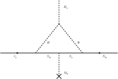
Figure 1: One-loop correction to the Dirac neutrino mass matrix.

A direct calculation results in

$$\left(M_{D}\right)_{ab}^{\rm loop}={\lambda_{n}\langle H_{n}\rangle\over 32\pi^{2}}\left(Y_{S}\right)_{ac}(Y_{N}^{\dagger})_{cb}M_{S_{c}}{\cal F}\left(M_{H}^{2},M_{\Phi}^{2},M_{S_{c}}^{2}\right)\;,$$ (8)

where the one loop function appearing in upper equation is given by

$${\cal F}(m_{1}^{2},m_{2}^{2},m^{2})={1\over m_{1}^{2}-m_{2}^{2}}\left({\ln\beta_{1}\over\beta_{1}-1}-{\ln\beta_{2}\over\beta_{2}-1}\right)\;,$$ (9)

with $\beta_{i}=m^{2}/m_{i}^{2}$. When $m_{1}=m_{2}=m$, ${\cal F}$ reduces to $1/2m^{2}$.

Here $M_{D}^{\rm loop}$ is the Dirac neutrino mass matrix linking the left and right hand neutrinos, which only raises at the loop level in our model. If neutrinos are Dirac particles, then Eq. (8) is just neutrino mass formula, whose predication must be consistent with present neutrino oscillation data. In this paper, we assume that neutrinos are Majorana particles, i.e., left-handed and right-handed neutrinos have different mass eigenvalues. Then three active neutrino masses can be generated from seesaw mechanism. In this case, we can write down the $6\times 6$ neutrino mass matrix:

$${\cal M}=\left(\matrix{0&M_{D}^{\rm loop}\cr M_{D}^{{\rm loop}T}&M_{R}}\right)\;,$$ (10)

which can be diagonalized by the unitary transformation ${\cal U}^{\dagger}{\cal M}{\cal U}^{*}=\widehat{{\cal M}}$; or explicitly,

$$\left(\matrix{V&R\cr S&T}\right)^{\dagger}\left(\matrix{0&M_{D}^{\rm loop}\cr M_{D}^{{\rm loop}T}&M_{R}}\right)\left(\matrix{V&R\cr S&T}\right)^{*}=\left(\matrix{\hat{M}_{\nu}{}&0\cr 0&\hat{M}_{N}}\right)\;.$$ (11)

Given $M_{D}^{\rm loop}\ll M_{R}$, the light Majorana neutrino mass formula is then $M_{\nu}=-M_{D}^{\rm loop}M_{R}^{-1}{M_{D}^{\rm loop}}^{T}$. Notice that Dirac neutrino mass matrix is suppressed by loop factor, we assume $M_{D}^{\rm loop}\sim{\cal O}(\rm MeV)$, which will not cause any fine-tune problem. Then, to generate electron-volt scale active neutrino masses, heavy Majorana neutrinos would be of the order of several hundred GeV.

We also obtain the charged lepton mass matrix in the basis $(E_{L},S_{L})^{T}$,

$$M_{\ell}=\left(\matrix{M_{E}&M_{C}\cr 0&M_{S}}\right)=\left(\matrix{\textbf{I}&M_{C}M_{S}^{-1}\cr 0&\textbf{I}}\right)\left(\matrix{M_{E}&0\cr 0&M_{S}}\right)\;,$$ (12)

where $M_{E}=v/\sqrt{2}Y_{E}$ and $M_{C}=v/\sqrt{2}Y_{S}$.

According to Eqs. (11) and (12), we may derive the lepton mixing matrix (MNS), which comes from the mismatch between the diagonalizations of the neutrino mass matrix and charged lepton mass matrix, i.e., $U=V_{e}^{\dagger}V_{\nu}$:

$$U\approx(\textbf{1}-{1\over 2}|M_{C}M_{S}^{-1}|^{2})V\;.$$ (13)

As a result, the effective charged and neutral current interactions for charged leptons can be written as

$$-{\cal L}_{\rm CC} \approx {g\over\sqrt{2}}\overline{e_{\alpha}}\gamma^{\mu}P_{L}U_{\alpha i}\nu_{i}W_{\mu}+{\rm h.c.}\;;$$ (14)

$$-{\cal L}_{\rm NC} \approx {g\over\cos\theta_{w}}\overline{e_{\alpha}}\gamma^{\mu}\left[(UU^{\dagger})_{\alpha\beta}(-{1\over 2}+\sin^{2}\theta_{w})P_{L}+\delta_{\alpha\beta}\sin^{2}\theta_{w}P_{R}\right]e_{\beta}Z_{\mu}\;.$$ (15)

The MNS matrix in Eq. (13) is non-unitary, which is mainly because the large mixing between charged leptons and heavy vector like fermions. To a better degree of accuracy, we have $UU^{\dagger}\approx\textbf{1}-|M_{C}M_{S}^{-1}|^{2}$. A global analysis of current neutrino oscillation data and precision electroweak data (e.g., on the invisible width of the $Z^{0}$ boson, universality tests and rare decays) has yield quite strong constraints on the unitarity of $U$. Translating the numerical results of Refs. zerodis ; extest1 ; zhizhong ; extest2 into the restriction on $|M_{C}M_{S}^{-1}|^{2}$, we have

$$|M_{C}M_{S}^{-1}|^{2}=\left(\matrix{<1.1\cdot 10^{-2}&<7.0\cdot 10^{-5}&<1.6\cdot 10^{-2}\cr<7.0\cdot 10^{-5}&<1.0\cdot 10^{-2}&<1.0\cdot 10^{-2}\cr<1.6\cdot 10^{-2}&<1.0\cdot 10^{-2}&<1.0\cdot 10^{-2}}\right)\;,$$ (16)

at the $90\%$ confidence level. In addition, interactions in Eqs. (14) and (15) will lead to tree level lepton flavor violations (as can be seen in Eq. (15)) and “ zero distance” effects zerodis in neutrino oscillations, which can be verified in the future long baseline neutrino oscillation experiments.

III.2 Lepton flavor violations (LFV)

Notice that the emergence of big unitary violation of MNS matrix can lead to observable LFV effects. In this subsection, we investigate constraints on parameter space from LFV processes.

In our model, $\ell_{i}\rightarrow 3\ell_{j}$ may occur at the tree level, just like the case in type III seesaw mechanism. The branching ratios for the $\mu\rightarrow 3e$ can be given by

$${\rm BR}(\mu\rightarrow e^{-}e^{+}e^{-})=|UU^{\dagger}|_{e\mu}^{2}\left[|UU^{\dagger}|_{ee}(-1+2\sin^{2}\theta_{w})^{2}+4\sin^{4}\theta_{w}\right]\Omega\;.$$ (17)

Here $\Omega$ is the final states phase space integration

$$\Omega=\int_{z_{d}}^{z_{u}}\sqrt{1-{4z_{0}\over z}}\left[-2z^{2}+(1+3z_{0})z-4z_{0}(1+z_{0})+{2z_{0}(1-z_{0})^{2}\over z}\right]\lambda^{1\over 2}(1,z_{0},z)dz\;,$$ (18)

where $z_{d}=4z_{0}$, $z_{u}=(1-\sqrt{z_{0}})^{2}$, $z_{0}=m_{e}^{2}/m_{\mu}^{2}$ and $\lambda(x,y,z)=x^{2}+y^{2}+z^{2}-2xy-2xz-2yz$.

Radiative decays, i.e., $\ell_{i}\rightarrow\ell_{j}+\gamma$ occur at one-loop level. The branching ratios for these processes can be written as

$${\rm BR}(\ell_{\beta}\rightarrow\ell_{\alpha}\gamma)={3\pi\alpha\over 16G_{\rm F}^{2}m_{\beta}^{4}}\left|\sum_{i}Y_{S\alpha i}Y_{S\beta i}^{*}{\cal S}_{i}\right|^{2}{\rm BR}(\ell_{\beta}\rightarrow\nu_{\beta}\ell_{\alpha}\bar{\nu}_{\alpha})\;,$$ (19)

with

$${\cal S}_{\rho}={\sqrt{z_{\alpha}z_{\beta}}(1-z_{h})-2z_{\beta}(1-z_{h})+2\sqrt{z_{\alpha}z_{\beta}}\over(1-z_{h})^{2}}-{z_{\beta}(1-z_{h})-\sqrt{z_{\alpha}z_{\beta}}\over(1-z_{h})^{3}}\ln z_{h}\;,$$ (20)

where $z_{\alpha}={m_{\alpha}^{2}/M_{Si}^{2}}\;;$ $z_{\beta}={m_{\beta}^{2}/M_{Si}^{2}}\;;$ $z_{h}={M_{h}^{2}/M_{Si}^{2}}\;.$

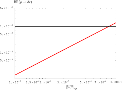
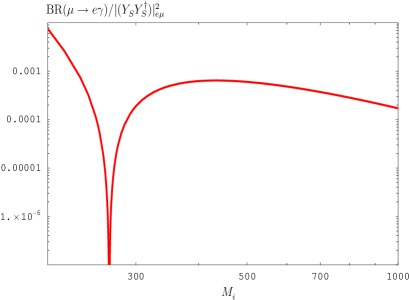
Figure 2: Branching ratios for (a) $\mu\rightarrow 3e$ and (b) $\mu\rightarrow e\gamma$.

In Fig. 2 (a), we plot ${\rm BR}(\mu\rightarrow 3e)$ as function of $|UU^{\dagger}|_{e\mu}^{2}$. The horizon line stands for current experimental constraints. Our result shows that, to meet the experimental data, $|UU^{\dagger}|_{e\mu}^{2}$ must lie below $8.5\times 10^{-6}$. Assuming that there is only one generation vector like fermion, we plot, in Fig. 2 (b), ${\rm BR}(\mu\rightarrow e\gamma)/|Y_{S}Y_{S}^{\dagger}|^{2}_{e\mu}$ as function of $M_{S}$ by setting $M_{h}=120~{}{\rm GeV}$. We find that, to get big Yukawa coupling $Y_{S}$, $M_{S}$ must lie around $270~{}{\rm GeV}$ or be heavier than several ${\rm TeV}$.

III.3 Electromagnetic properties of heavy Majorana neutrinos

The electromagnetic properties of Majorana neutrinos show up, in a quantum field theory, as its interaction with the photon, and is described by the following effective interaction vertex: ${\cal L}_{\rm eff}=\bar{\psi}\Gamma_{\mu}\psi A^{\mu}$. The most general matrix element of ${\cal L}_{\rm eff}$ between two one-particle states, i.e., $\langle p^{\prime},s^{\prime}|J_{\mu}(0)|p,s\rangle=\bar{u}_{s^{\prime}}(p^{\prime})\Gamma_{\mu}u_{s}(p)$, which is consistent with the Lorentz invariance, can be written as

$$\bar{u}(p_{2},s_{2})\Gamma^{\mu}u(p_{1},s_{1})=\bar{u}(p_{2},s_{2})\left[{\cal E}(q^{2})\gamma^{\mu}-{\cal M}(q^{2})i\sigma^{\mu\nu}q^{\nu}+{\cal H}(q^{2})q^{\mu}\right]u(p_{1},s_{1})$$

$$+\bar{u}(p_{2},s_{2})\left[{\cal G}(q^{2})\gamma^{\mu}\gamma^{5}-{\cal T}(q^{2})i\sigma^{\mu\nu}q^{\nu}\gamma^{5}+{\cal S}(q^{2})q^{\mu}\gamma^{5}\right]u(p_{1},s_{1}) \;,$$ (21)

where $q=p_{2}-p_{1}$. $2M{\cal M}(0)$ and $2M{\cal T}(0)$ correspond to the magnetic moment and electro dipole moment of heavy neutrinos, respectively.

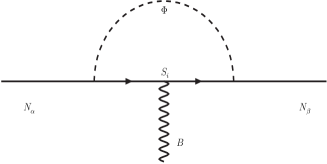
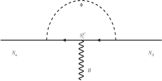
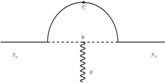
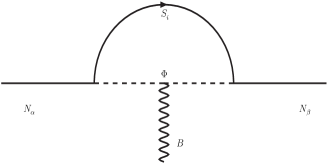
Figure 3: Feynman diagrams contributing to heavy Majorana neutrino transition magnetic moment.

Due to the Majorana nature, the magnetic moment of heavy Majorana neutrinos is zero. There is only transition magnetic moment for them. In the model considered, we have four diagrams contributing to the transition magnetic moment, which are depicted in Fig. 3. The Yukawa interactions of heavy Majorana neutrinos with $\Phi$ and $S$ can be rewritten in the following way

$${1\over 2}\left[\overline{N^{C}_{\alpha}}\Phi^{-}(Y^{T})_{\alpha i}P_{R}S_{i}^{C}+\overline{N_{\alpha}}\Phi^{+}(Y^{\dagger})_{\alpha i}P_{L}S_{i}\right]+{1\over 2}\left[\overline{S_{i}}Y_{i\alpha}\Phi^{-}P_{R}N_{\alpha}+\overline{S_{i}^{C}}(Y^{*})_{i\alpha}\Phi^{+}P_{L}N_{\alpha}^{C}\right]\;,$$ (22)

through which we can derive relevant feynman rules. Assuming that heavy Majorana neutrinos are nearly degenerate, i.e., $M_{\alpha}\approx M_{\beta}\approx M$, we derive the transition magnetic moment for heavy Majorana neutrinos

$${a}_{\alpha\beta}^{N}={M^{2}\over 64\pi^{2}}\left[(Y_{N}^{\dagger})_{\beta i}(Y_{N})_{i\alpha}-(Y_{N}^{T})_{\beta i}(Y_{N})_{i\alpha}^{*}\right]\left[{\cal I}(M_{\Phi}^{2},M^{2},M_{i}^{2})-{\cal I}(M_{i}^{2},M^{2},M_{\Phi}^{2})\right]\;,$$ (23)

with

$${\cal I}(A,B,C)=\int dx{x(1-x)^{2}\over(1-x)A+x(x-1)B+xC}\;,$$

where $M_{i}$ and $M_{\Phi}$ are the mass eigenvalues of heavy vector-like fermion $S$ and scalar $\Phi$, respectively.

Now, we turn to some numerical analysis. As shown in Eq. (2), $Y_{N}\overline{S_{L}}\Phi N_{R}$ is totally the interaction of new fields beyond the SM, so that there is no experimental constraint on $Y_{N}$ except ${\cal O}(Y_{N})<\sqrt{4\pi}$ (to satisfy the perturbation theory). We plot, in Fig. 4, $|a_{\alpha\beta}^{N}/[(Y_{N}^{\dagger})_{\beta i}(Y_{N})_{i\alpha}-(Y_{N}^{T})_{\beta i}(Y_{N})_{i\alpha}^{*}]|$ as function of $M_{N}$. Assuming ${\cal O}([(Y_{N}^{\dagger})_{\beta i}(Y_{N})_{i\alpha}-(Y_{N}^{T})_{\beta i}(Y_{N})_{i\alpha}^{*}])\sim 1$, We can find that the transition magnetic moment of heavy Majorana neutrinos can be of ${\cal O}(10^{-2})$ for special parameter settings. Our result in Eq. (23) is different from that in Ref. wudka2 for not considering the Yukawa coupling $\overline{N_{R}^{C}}\Phi S_{R}$, which is forbidden by the $Z_{2}$ symmetry in our model. Given the large electromagnetic form factors, heavy Majorana neutrinos can be produced at the LHC through the electromagnetic interaction.

Figure 4: Numerical illustration for the transition magnetic moment of heavy Majorana neutrinos as function of $M_{N}$. We assume there is only one generation vector-like fermion $S$ and choose $(M_{\Phi},~{}M_{i})=(350,~{}150)~{}({\rm GeV})~{}$for solid line, $(300,~{}200)~{}({\rm GeV})$ for dashed line and $(300,~{}250)~{}({\rm GeV})$ for dotted line.

III.4 Collider signatures

We switch to comment on the collider signatures of our model. All of the new particles introduced in the model lie around several hundred GeV. Singly charged scalar and vector like fermions can be produced through the electromagnetic interaction at the LHC. The most promising production channel may be $pp\rightarrow S^{+}S^{-}\rightarrow\ell^{+}\ell^{-}jjjj$ for heavy charged fermions and $pp\rightarrow\Phi^{+}\Phi^{-}\rightarrow jjjj$ for heavy charged scalar. The production cross sections for these charged particles at the LHC (with $\sqrt{s}=14{\rm TeV}$) are about several $fb$ when heavy particle masses lie around 300 GeV wudka1 ; wudka2 . The large transition magnetic moment can help to produce the heavy Majorana neutrinos at the LHC. Its signatures are similar to that in Type-III seesaw model tripletp1 ; tripletp2 ; tripletp3 . The only distinguish is that, heavy neutrinos can not be produced through weak interactions and must be produced in pair in our model.

IV concluding remarks

In this paper, we have proposed a novel TeV-scale seesaw mechanism. One salient feature of our model is that Dirac neutrino mass matrix raises only at the loop level. As a result, the heavy Majorana neutrinos can be several hundred GeV. Another salient feature is that heavy Majorana neutrinos can get large electromagnetic form factors, through which they can be produced and detected at the LHC. We have derived light Majorana neutrino mass formula and calculated constraints on parameter space from LFV processes. At last we have discussed the signatures of heavy fermions (vector-like fermions and heavy Majorana neutrinos) and scalar at the LHC.

Appendix A An alternative setting to the model

Beside the model presented in section II, we can extending the SM with different particle contents, which may lead to the same TeV seesaw mechanism. For example, we can substitute $S_{L},S_{R}$, $\Phi$, with vector like fermion triplets $\Sigma_{L},\Sigma_{R}$ and scalar triplet $\Delta$. In this case the lagrangian can be written as

$${\cal L}={\cal L}_{\rm SM}-\overline{\ell_{L}}Y_{\Psi}\tilde{H}\Sigma_{R}-\overline{\Sigma_{L}}M_{\Sigma}\Sigma_{R}-Y_{N}{\rm Tr}[\Psi_{L}\Delta]N_{R}+V(H,\Delta)\;.$$ (24)

Here the weak hypercharge of the $\Psi$ and $\Sigma$ are zero. $\Psi_{L}$, $\Phi$ and $N_{R}$ are odd , while the other fields are even under $Z_{2}$ transformation.

The Higgs potential can be written as

$$V = {1\over 2}m_{H}^{2}H^{\dagger}H+{1\over 2}m_{\Delta}{\rm Tr}[\Delta^{\dagger}\Delta]+{1\over 4}\lambda(H^{\dagger}H)^{2}+\lambda_{X}H^{\dagger}\Sigma i\sigma_{2}H+\cdots\;,$$ (25)

where dots denote Higgs potential terms we don’t concern.

References

- (1) SNO Collaboration, Q. P. Ahamed et al., Phys. Rev. Lett. 89, 011301 (2002).
- (2) For a review, see: C. K. Jung et al., Ann. Rev. Nucl. Part. Sci. 51, 451 (2001).
- (3) KamLAND Collaboration, K. Eguchi et al., Phys. Rev. Lett. 90, 021802 (2003).
- (4) K2K Collaboration, M. H. Ahn et al., Phys. Rev. Lett. 90, 041801 (2003).
- (5) S. Weinberg, Phys. Rev. Lett. 43, 1566 (1979).
- (6) P. Minkowski, Phys. Lett. B 67, 421 (1977); T. Yanagida, in Workshop on Unified Theories, KEK report 79-18 p.95 (1979); M. Gell-Mann, P. Ramond, R. Slansky, in Supergravity (North Holland, Amsterdam, 1979) eds. P. van Nieuwenhuizen, D. Freedman, p.315; S. L. Glashow, in 1979 Cargese Summer Institute on Quarks and Leptons (Plenum Press, New York, 1980) eds. M. Levy, J.-L. Basdevant, D. Speiser, J. Weyers, R. Gastmans and M. Jacobs, p.687; R. Barbieri, D. V. Nanopoulos, G. Morchio and F. Strocchi, Phys. Lett. B 90, 91 (1980); R. N. Mohapatra and G. Senjanovic, Phys. Rev. Lett. 44, 912 (1980); G. Lazarides, Q. Shafi and C. Wetterich, Nucl. Phys. B 181, 287 (1981).
- (7) W. Konetschny and W. Kummer, Phys. Lett. B 70, 433 (1977); T. P. Cheng and L. F. Li, Phys. Rev. D 22, 2860 (1980); G. Lazarides, Q. Shafi and C. Wetterich, Nucl. Phys. B 181, 287 (1981); J. Schechter and J. W. F. Valle, Phys. Rev. D 22, 2227 (1980); R. N. Mohapatra and G. Senjanovic, Phys. Rev. D 23, 165 (1981).
- (8) R. Foot, H. Lew, X. G. He and G. C. Joshi, Z. Phys. C 44, 441 (1989).
- (9) E. Ma and U. Sarkar, Phys. Rev. Lett. 80, 5716 (1998).
- (10) M. Y. Keung and G. Senjanovic, Phys. Rev. Lett. 50, 1427 (1983); A. Pilaftsis, Z. Phys. C 55, 275 (1992); B. Bajc, M. Nemevsek and G. Senjanovic, Phys. Rev. D 76, 055011 (2007).
- (11) J. Bernabeu, A. Santamaria, J. Vidal, A. Mendez, and J.W.F. Valle, Phys. Lett. B 187, 303 (1987); W. Buchmuller and D. Wyler, Phys. Lett. B 249, 458 (1990); W. Buchmuller and C. Greub, Nucl. Phys. B 363, 345 (1991); A. Datta and A. Pilaftsis, Phys. Lett. B 278, 162 (1992); G. Ingelman and J. Rathsman, Z. Phys. C 60, 243 (1993); C.A. Heusch and P. Minkowski, Nucl. Phys. B 416, 3 (1994); D. Tommasini, G. Barenboim, J. Bernabeu, and C. Jarlskog, Nucl. Phys. B 444, 451 (1995).
- (12) J. Gluza, Acta Phys. Polon. B 33, 1735 (2002); J. Kersten and A.Yu Smirnov, Phys. Rev. D 76, 073005 (2007); X. G. He, S. Oh, J. Tandean and C. C. Wen, Phys. Rev. D 80, 073012 (2009).
- (13) T. Han and B. Zhang, Phys. Rev. Lett. 97, 171804 (2006).
- (14) F.del Aguila, J.A. Aguilar-Saavedra, A.M. de la Ossa, and M. Meloni, Phys. Lett. B 613, 170 (2005); F.del Aguila and J.A. Aguilar-Saavedra, JHEP 0505, 026 (2005); F.del Aguila, J. A. Aguilar-Saavedra, and R. Pittau, JHEP 0710, 047 (2007); N. Haba, S. Matsumoto and K. Yoshioka, Phys. Lett. B 677, 291 (2009).
- (15) W. Chao, S. Luo, Z.Z. Xing, and S. Zhou, Phys. Rev. D 77, 016001 (2008); W. Chao, Z. Si, Z.Z. Xing, and S. Zhou, Phys. Lett. B 666, 451 (2008); Z. Z. Xing, Phys. Lett. B 679, 255 (2009); W. Chao, Z. Si, Y. J. Zheng and S. Zhou, Phys. Lett. B 683, 26 (2010).
- (16) A. Zee, Phys. Lett. B 93, 389 (1980), Erratum-ibid.B 95, 461 (1980).
- (17) S. Antusch, C. Biggio, E. Fernandez-Martinez, M. B. Gavela and J. Lopez-Pavon, JHEP 0610, 084 (2006).
- (18) E. Fernandez-Martinez, M. B. Gavela, J. Lepez-Pavon and O. Yasuda, Phys. Lett. B 649, 427 (2007).
- (19) Z. Z. Xing, Phys. Lett. B 660, 515 (2008).
- (20) A. Abada, C. Biggio, F. Bonnet, B. Gavela and T. Hambye, JHEP, 0712, 061 (2007).
- (21) A. Aparici, K. Kim, A. Santamaria and J. Wudka, Phys. Rev. D 80, 013010 (2010).
- (22) A. Aparici, K. Kim, A. Santamaria and J. Wudka, arXiv: 0911.4103 [hep-ph].
- (23) R. Franceschini, T. Hambye and A. Strumia, Phys. Rev. D 78, 033002 (2008).
- (24) F. del Agulia and J. A. Aguilar-Saavedra, Nucl. Phys. B 813, 22 (2009).
- (25) Tong Li and X. G. He, Phys. Rev. D 80. 093003 (2009).