Many-body interactions and nuclear structure

Abstract

This article presents several challenges to nuclear many-body theory and our understanding of the stability of nuclear matter. In order to achieve this, we present five different cases, starting with an idealized toy model. These cases expose problems that need to be understood in order to match recent advances in nuclear theory with current experimental programs in low-energy nuclear physics.

In particular, we focus on our current understanding, or lack thereof, of many-body forces, and how they evolve as functions of the number of particles. We provide examples of discrepancies between theory and experiment and outline some selected perspectives for future research directions.

1 Introduction

A central issue in basic nuclear physics research is to understand the limits of stability of matter starting from its basic building blocks, either represented by effective degrees of freedom such as various hadrons or employing the underlying theory of the strong interaction, namely quantum chromodynamics. To achieve this implies the development of a comprehensive description of all nuclei and their reactions, based on a strong interplay between theory and experiment. This interplay should match the research conducted at present and planned experimental facilities, where one of the aims is to study unstable and rare isotopes. These nuclei can convey crucial information about the stability of nuclear matter, but are difficult to produce experimentally since they can have extremely short lifetimes. They exhibit also unsual neutron-to-proton ratios that are very different from their stable counterparts. Furthermore, these rare nuclei lie at the heart of nucleosynthesis processes in the universe and are therefore an important component in the puzzle of matter generation in the universe.

We do expect that these facilities will offer unprecendeted data on weakly bound systems and the limits of stability. To interpret such a wealth of experimental data and point to new experiments that can shed light on various properties of matter requires a reliable and predictive theory. If a theoretical model is capable of explaining a wealth of experimental data, one can thereafter analyze the results in terms of specific components of, say, the nuclear forces and extract simple physics pictures from complicated many-body systems.

To better understand the rationale for this article, it is important to keep in mind the particularity of nuclear physics. Basic nuclear physics research, as conducted today, is very diverse in nature, with experimental facilities which include accelerators, reactors, and underground laboratories. This diversity reflects simply the rather complex nature of the nuclear forces among protons and neutrons. These generate a broad range and variety in the nuclear phenomena that we observe, from energy scales of several gigaelectronvolts (GeV) to a few kiloeletronvolts (keV). Nuclear physics is thus a classic example of what we would call multiscale physics. The many scales pose therefore a severe challenge to nuclear many-body theory and what are dubbed ab initio descriptions  of nuclear systems. Examples of key physics issues which need to be addressed by nuclear theory are:

• How do we derive the in-medium nucleon-nucleon interaction from basic principles?

• How does the nuclear force depend on the proton-to-neutron ratio?

• What are the limits for the existence of nuclei?

• How can collective phenomena be explained from individual motion?

• Can we understand shape transitions in nuclei?

In order to deal with the above-mentioned problems from an ab initio standpoint, it is our firm belief that nuclear many-body theory needs to meet some specific criteria in order to be credible. Back in 2004 two of the present authors co-authored a preface to a collection of articles from a workshop on many-body theories, see Ref. [1] for more details. Seven specific requirements to theory were presented. These were:

• A many-body theory should be fully microscopic and start with present two- and three-body interactions derived from, e.g., effective field theory;

• The theory can be improved upon systematically, e.g., by inclusion of three-body interactions and more complicated correlations;

• It allows for a description of both closed-shell systems and valence systems;

• For nuclear systems where shell-model studies are the only feasible ones, viz., a small model space requiring an effective interaction, one should be able to derive effective two- and three-body equations and interactions for the nuclear shell model;

• It is amenable to parallel computing;

• It can be used to generate excited spectra for nuclei like where many shells are involved. (It is hard for the traditional shell model to go beyond one major shell. The inclusion of several shells may imply the need of complex effective interactions needed in studies of weakly bound systems); and

• Finally, nuclear structure results should be used in marrying microscopic many-body results with reaction studies. This will be another hot topic of future ab initio research.

Six years have elapsed since these requirements were presented. Recent advances in nuclear theory have made redundant most of the points listed above. They are actually included in many calculations, either fully or partly. On the other hand, in the last five years, we have witnessed considerable progress in nuclear theory. Of relevance to this article are the developments of effective field theories [2, 3], lattice quantum chromodynamics calculations, with the possibility to constrain specific parameters of the nuclear forces [4, 5, 6] and of many-body theories applied to nuclei, see for example Refs. [7, 8, 9, 10]. There are also several efforts to link standard ab initio methods with density functional theories, or more precisely, energy density functional theories, see Refs. [11, 12, 13].

These developments have led us to formulate some key intellectual issues and further requirements we feel nuclear theory needs to address. The key issues are:

1. Is it possible to link lattice quantum chromodynamics calculations with effective field theories in order to better understand the nuclear forces to be used in a many-body theory?

2. A nuclear force derived from effective field theory is normally constructed with a specific cutoff in energy or momentum space. Most interactions have a cutoff $\Lambda$ in the range $\Lambda\sim 500$-$600$ MeV. The question we pose here is how well do we understand the link between this cutoff and a specific Hilbert space (the so-called model space) used in a many-body calculation?

3. The last question is crucially linked with our understanding of many-body forces and leads us to the next question. Do we understand how many-body forces evolve as we add more and more particles? Irrespective of whether our Hamiltonian contains say two- and three-body interactions, a truncated Hilbert space results in missing many-body correlations. To understand how these correlations evolve as a function of the number of particles is crucial in order to provide a predictive many-body theory.

4. Finally, in order to deal with systems beyond closed-shell nuclei with or without some few valence nucleons, we need to link ab initio methods with density functional theory.

With respect to requirements, we find it timely to request that a proper many-body theory should provide uncertainty quantifications. For most methods, this means to provide an estimate of the error due to the truncation made in the single-particle basis and the truncation made in limiting the number of possible excitations. The first point, as shown by Kvaal [14], can be rigorously proven for a chosen single-particle basis. The second point is more difficult and is normally justified a posteriori. As an example, in coupled-cluster calculations, a truncation is made in terms of various particle-hole excitations. Only specific sub-clusters of excitations are included to infinite order, see for example Ref. [15]. Whether this subset of excitations is sufficient or not can only be justified after the calculations have been performed.

This article does not aim at answering the above questions. Rather, our goal is to raise the awareness about these issues since it is our belief that they can lead to a more predictive nuclear many-body theory. Our focus is on the third topic, and we illustrate the problems which can arise via a simple toy model in Section 2. Thereafter, we discuss four possible physics cases where the effect of missing many-body forces can be studied theoretically and benchmarked through existing and planned experiments. The physics cases are all linked with studies of isotopic chains of nuclei, with several closed-shell nuclei accessible to ab initio calculations. Our physics cases are discussed in Section 3. We start with the chain of oxygen isotopes, from ¹⁶O to ²⁸O. The next cases deal with isotopes in the $pf$ shell, namely the Ni isotopes (⁴⁸Ni, ⁵⁶Ni, ⁶⁸Ni, and ⁷⁸Ni) and the Ca isotopes (⁴⁰Ca, ⁴⁸Ca, ⁵²Ca, ⁵⁴Ca, and ⁶⁰Ca). We conclude with the chain of tin isotopes from ¹⁰⁰Sn to ¹⁴⁰Sn. For isotopes like ²⁸O, ⁵⁴Ca, ⁶⁰Ca, and ¹⁴⁰Sn, data on binding energies are missing. We try to give here a motivation why one should attempt to measure these nuclei.

Our conclusions and perspectives are presented in the last section.

2 A simple toy model

We start with a model described by a simple two-body Hamiltonian. This model catches the basic features concerning the connection between many-body forces and the size of the model space. In particular we will stress the link between a given effective Hilbert space and missing many-body effects. This section, although it forms the largest part of this article, conveys the problems which can arise in many-body calculations with truncated spaces and effective interactions.

The model we present mimicks the effects seen in standard shell-model calculations with an effective interaction, either with a valence model space [16] or a so-called no-core model space [8].

2.1 Hamiltonian

The Hamiltonian acting in the complete Hilbert space (usually infinite dimensional) consists of an unperturbed one-body part, $\hat{H}_{0}$, and a perturbation $\hat{V}$. The goal is to obtain an effective interaction $\hat{V}_{\mathrm{eff}}$ acting in a chosen model or valence space. By construction, it gives a set of eigenvalues which are identical to (a subset of) those of the complete problem.

If we limit ourselves to, at most, two-body interactions, our Hamiltonian is then represented by the following operators

$$\hat{H}=\sum_{\alpha\beta}\langle\alpha|h_{0}|\beta\rangle a_{\alpha}^{\dagger}a_{\beta}+\frac{1}{4}\sum_{\alpha\beta\gamma\delta}\langle\alpha\beta|V|\gamma\delta\rangle a_{\alpha}^{\dagger}a_{\beta}^{\dagger}a_{\delta}a_{\gamma},$$

where $a_{\alpha}^{\dagger}$ and $a_{\alpha}$, etc. are standard fermion creation and annihilation operators, respectively, and $\alpha\beta\gamma\delta$ represent all possible single-particle quantum numbers. The full single-particle space is defined by the completeness relation $\hat{{\bf 1}}=\sum_{\alpha=1}^{\infty}|\alpha\rangle\langle\alpha|$. In our calculations we will let the single-particle states $|\alpha\rangle$ be eigenfunctions of the one-particle operator $\hat{h}_{0}$.

The above Hamiltonian acts in turn on various many-body Slater determinants constructed from the single-basis defined by the one-body operator $\hat{h}_{0}$. We can then diagonalize a two-body problem in a large space and project out via a similarity transformation an effective two-body interaction. The interaction acts in a much smaller set of single-particle states. The two-particle model space $\mathcal{P}$ is defined by an operator

$$\hat{P}=\sum_{\alpha\beta=1}^{m}|\alpha\beta\rangle\langle\alpha\beta|,$$

where we assume that $m=\dim(\mathcal{P})$ and the full space is defined by

$$\hat{P}+\hat{Q}=\hat{{\bf 1}}.$$

Our specific model consists of $N$ doubly degenerate and equally spaced single-particle levels labelled by $p=1,2,\dots$ and spin $\sigma=\pm 1$. These states are schematically portrayed in Fig. 1. The first five single-particle levels define a possible model space indicated by the label $\mathcal{P}$.

We write the Hamiltonian as

$$\hat{H}=\hat{H}_{0}+\hat{V},$$

where

$$\hat{H}_{0}=\xi\sum_{p\sigma}(p-1)a_{p\sigma}^{\dagger}a_{p\sigma}$$

and

$$\hat{V}=-\frac{1}{2}g\sum_{pq}a^{\dagger}_{p+}a^{\dagger}_{p-}a_{q-}a_{p+}-\frac{1}{2}f\sum_{pqr}\left(a^{\dagger}_{p+}a_{p-}^{\dagger}a_{q-}a_{r+}+\mathrm{h.c.}\right).$$

Here, $H_{0}$ is the unperturbed Hamiltonian with a spacing between successive single-particle states given by $\xi$, which we may set to a constant value $\xi=1$ without loss of generality. The two-body operator $\hat{V}$ has two terms. The first term represents the pairing contribution and carries a constant strength $g$. (It easy to extend our model to include a state dependent interaction.) The indices $\sigma=\pm$ represent the two possible spin values. The first term of the interaction can only couple pairs and excites therefore only two particles at the time, as indicated by the rightmost four-particle state in Fig. 1. There, a pair is excited to the state with $p=9$. The second interaction term, carrying a constant strength $f$, acts between a set of particles with opposite spins and allows for the breaking of a pair or just to excite a single-particle state. The spin of a given single-particle state is not changed. This interaction can be interpreted as a particle-hole interaction if we label single-particle states within the model space as hole-states. The single-particle states outside the model space are then particle states.

In our model we have kept both the interaction strength and the single-particle level as constants. In a realistic system like a nucleus, this is not the case; however, if a harmonic oscillator basis is used, as done in the no-core shell-model calculations [8], at least the single-particle basis mimicks the input to realistic calculations.

Figure 1: Schematic plot of the possible single-particle levels with double degeneracy. The filled circles indicate occupied particle states while the empty circles represent vacant particle(hole) states. The spacing between each level $p$ is constant in this picture. The first five single-particle levels define a possible model space, indicated by the label $\mathcal{P}$. The remaining states span the excluded space $\mathcal{Q}$. The first state to the left represents a possible ground state representation for a four-fermion system. In the second state to the left, one pair is broken by the interaction. All single-particle orbits belong to the model space. The two remaining four-particle states represents single-particle excitations to the excluded space, either by breaking two pairs or breaking one pair and exciting one pair (rightmost state).

2.2 Effective Hamiltonians

We now consider a general $A$-body situation, of which our model is just an example, where a Hilbert space of finite dimension $n$ is given along with an $A$-body Hamiltonian $\hat{H}$ with spectral decomposition given by

$$\hat{H}=\sum_{k=1}^{n}E_{k}|\psi_{k}\rangle\langle\psi_{k}|,$$

where $\{|\psi_{k}\rangle\}_{k=1}^{n}$ is an orthonormal basis of eigenvectors and where $E_{k}$ are the corresponding eigenvalues. We choose the dimension $n$ to be finite for simplicity, but the theory may be generalized to infinite dimensional settings where $\hat{H}$ has a purely discrete spectrum.

The Hilbert space is divided into the model space $\mathcal{P}$ and its complement, denoted by $\mathcal{Q}$. We assume again that $m=\dim(\mathcal{P})$.

The effective Hamiltonian $\hat{H}_{\mathrm{eff}}$ is defined in the $\mathcal{P}$-space only, and by definition its eigenvalues are identical to the $m$ eigenvalues of $\hat{H}$. This is equivalent to $\hat{H}_{\mathrm{eff}}$ being given by

$$\hat{H}_{\mathrm{eff}} := \hat{P}\mathcal{H}\hat{P}$$

$$= \hat{P}e^{-\hat{G}}\hat{H}e^{\hat{G}}\hat{P},$$

where $\mathcal{H}$ is assumed to obey the de-coupling equation

$$\hat{Q}\mathcal{H}\hat{P}=0.$$

If the latter is satisfied, the $\mathcal{P}$-space is easily seen to be invariant under $\mathcal{H}$, and since similarity transformations preserve eigenvalues, $\hat{H}_{\mathrm{eff}}$ is seen to have $m$ eigenvalues of $\hat{H}$.

Without loss of generality, we assume that the eigenvalues $E_{k}$ of $\hat{H}$ are arranged so that $\hat{H}_{\mathrm{eff}}$, which is non-Hermitian in general, has the spectral decomposition

$$\hat{H}_{\mathrm{eff}}=\sum_{k=1}^{m}E_{k}|\phi_{k}\rangle\tilde{\langle\phi_{k}|},$$

where $\{|\phi_{k}\rangle\}_{k=1}^{m}$ is a basis for the $\mathcal{P}$-space, and where $\langle\phi_{k}|\tilde{\phi_{\ell}}\rangle=\delta_{k,\ell}$ defines the bi-orthogonal basis $\{|\tilde{\phi}_{k}\rangle\}_{k=1}^{m}$.

The similarity transform operator $\exp(\hat{G})$ is, of course, not unique; $E_{k}$, $k=1,\cdots,m$ can be chosen in many ways, and even if the effective eigenvector $|\phi_{k}\rangle$ is chosen to be related to $|\psi_{k}\rangle$, there is still great freedom of choice left.

Assume that we have determined the eigenvalues $E_{k}$, $k=1,\ldots,m$ that $\hat{H}_{\mathrm{eff}}$ should have. Two choices of the corresponding $|\phi_{k}\rangle$ are common: The Bloch-Brandow choice, and the canonical Van Vleck choice, resulting in “the non-Hermitian” and “the Hermitian” effective Hamiltonians, respectively. For a discussion of these approaches see Refs. [17, 18, 19, 20, 21, 22, 23, 24].

In the Bloch-Brandow scheme, the effective eigenvectors are simply chosen as

$$|\phi_{k}\rangle:=\hat{P}|\psi_{k}\rangle,$$

which gives meaning whenever $\hat{P}|\psi_{k}\rangle$ defines a basis for $\mathcal{P}$-space. In this case, $\hat{G}=\hat{\omega}$, where $\hat{\omega}=\hat{Q}\hat{\omega}\hat{P}$, defined by

$$\hat{\omega}\hat{P}|\psi_{k}\rangle:=\hat{Q}|\psi_{k}\rangle,\quad k=1,\cdots,m.$$

In contrast, the canonical Van Vleck effective Hamiltonian chooses a certain orthogonalization of $\{\hat{P}|\psi_{k}\rangle\}_{k=1}^{m}$ as effective eigenvectors [25]. In this case, $\hat{G}=\mathrm{arctanh}(\hat{\omega}-\hat{\omega}^{\dagger})$, which relates the two effective Hamiltonians to each other. The canonical effective interaction $\hat{H}_{\mathrm{eff}}$ minimizes the quantity $\Delta$ defined by

$$\Delta(|\chi_{1}\rangle,\cdots,|\chi_{m}\rangle):=\sum_{k=1}^{m}\||\chi_{k}\rangle-|\psi_{k}\rangle\|^{2},$$ (1)

where the minimum is taken with respect to all orthonormal sets of $\mathcal{P}$-space vectors $\chi$. In fact, it can be taken as the definition [25]. The Bloch-Brandow effective eigenvectors, on the other hand, yield the global minimum of $\Delta$.

We have not yet specified which of the eigenvalues of $H$ is to be reproduced by $\hat{H}_{\mathrm{eff}}$. In general, we would like it to reproduce the ground state and the other lowest eigenstates of $H$ if $m>1$. We consider this question in some detail in the following sections.

But first, we define the effective interaction $\hat{V}_{\mathrm{eff}}$ as

$$\hat{V}_{\mathrm{eff}}:=\hat{H}_{\mathrm{eff}}-\hat{P}\hat{H}_{0}\hat{P},$$

where $[\hat{H}_{0},\hat{P}]=0$ is assumed. This is satisfied whenever the model space is spanned by Slater determinants being eigenvectors of $\hat{H}_{0}$, such as in the model studied in this article.

Finding $\hat{H}_{\mathrm{eff}}$ is equivalent to solving the original problem. In order to be useful, we need some sort of approximation scheme to find $\hat{H}_{\mathrm{eff}}$. It is common to use many-body perturbation techniques such as folded diagrams [16], but as these suffer from convergence problems, the no-core shell model community [8] has developed the so-called sub-cluster approximation to $\hat{V}_{\mathrm{eff}}$. This is a non-perturbative approach, and utilizes the many-body nature of $\hat{H}$. The resulting effective interaction is often referred to as the Lee-Suzuki effective interaction [26].

In our model, $\mathcal{P}$ is defined by restricting the allowed levels accessible for the $A$ particles under study. Thus,

$$\mathcal{P}^{(A)}:=\left\{|(p_{1},\sigma_{1})\cdots(p_{A},\sigma_{A})\rangle\;:\;p_{k}\leq N_{P}\right\},$$

where $N_{P}\leq N$ is the number of levels accessible in the model space. This is the way model spaces in general are built up, simply restricting the single-particle orbitals accessible. It is by no means the only possible choice. On the other hand, this way of defining the model space has a very intuitive appeal, as it naturally leads to a view of $\hat{H}_{\mathrm{eff}}$ as a renormalization of $\hat{H}$. It also gives a natural relation between model spaces for different $A$, which is absolutely necessary for the sub-cluster effective Hamiltonian to be meaningful.

The effective Hamiltonian is seen to be an $A$-body operator in general, even though $H$ itself may contain only two-body operators. Thus, $\hat{V}_{\mathrm{eff}}$ can be written in its most general form as

$$\hat{V}^{(A)}_{\mathrm{eff}}=\sum_{\alpha_{1},\cdots,\alpha_{A}}\sum_{\beta_{1},\cdots,\beta_{A}}u^{\alpha_{1},\cdots}_{\beta_{1},\cdots}a^{\dagger}_{\alpha_{1}}\cdots a^{\dagger}_{\alpha_{A}}a_{\beta_{A}}\cdots a_{\beta_{1}},$$

where $\alpha_{k}=(p_{k},\sigma_{k})$ and $u^{\alpha_{1},\cdots}_{\beta_{1},\cdots}$ represent a specific matrix element. The approximation idea is then to obtain instead an $a$-body effective interaction $\hat{V}_{\mathrm{eff}}^{(a)}$, where $a<A$, and view this as an approximation to $\hat{V}_{\mathrm{eff}}^{(A)}$. This leads to

$$\hat{V}^{(A)}_{\mathrm{eff}}\approx\frac{\left(\begin{array}[]{c}A\\ 2\end{array}\right)}{\left(\begin{array}[]{c}A\\ a\end{array}\right)\left(\begin{array}[]{c}a\\ 2\end{array}\right)}\hat{V}^{(a)}_{\mathrm{eff}},$$

which is a much simpler operator, usually obtainable exactly by large-scale diagonalization of the $a$-body Hamiltonian.

The remaining question is which eigenpairs of $H^{(a)}$ should be reproduced by $\hat{H}_{\mathrm{eff}}^{(a)}$, and which approximate eigenvectors should be used. There is no unique answer to this. The “best” answer would be for each problem to require a complete knowledge of the conserved observables of the many-body Hamiltonian [14, 25].

On the other hand, if $\hat{V}$ is a small perturbation, that is, we let $\hat{V}\mapsto\lambda\hat{V}$ and consider an adiabatic turning on by slowly increasing $\lambda$, then it is natural to choose the eigenvalues developing adiabatically from $\lambda=0$. Indeed, $\hat{V}_{\mathrm{eff}}^{(a)}$ is then seen to be identical to a class of $a$-body terms in the perturbation series for the full $\hat{V}_{\mathrm{eff}}^{(A)}$ to infinite order [23, 24]. The problem is, there is no way in general to decide which eigenvalues have developed adiabatically from $\lambda=0$, and we must resort to a heuristic procedure.

Two alternatives present themselves as obvious candidates: Selecting the smallest eigenvalues, and selecting the eigenvalues whose eigenvectors have the largest overlap $\langle\psi_{k}|P|\psi_{k}\rangle$ with $\mathcal{P}$. Both are equivalent for sufficiently small $\lambda$, but the eigenvalues will cross in the presence of so-called intruder states for larger $\lambda$ [27, 28, 29]. Moreover, the presence of perhaps unknown constants of motion will make the selection by eigenvalue problematic, as exact crossings may lead us to select eigenpairs with $\hat{P}|\psi_{k}\rangle=0$, which makes $\hat{H}_{\mathrm{eff}}^{(a)}$ ill-defined. We therefore consider selection by model space overlap to be more robust in general. These considerations are, however, not important for our main conclusions.

The non-Hermitian Bloch-Brandow effective Hamiltonian runs into problems in the sub-cluster approach since the interpretation of $\hat{V}_{\mathrm{eff}}^{(a)}$ as an interaction requires hermiticity when applied to an $A$-body problem – otherwise, eigenvalues will be complex unless $a=A$.

See Ref. [25] for details on the algorithm for computing the effective interactions.

2.3 Pure pairing interaction

We first set $f\equiv 0$, giving a pure pairing Hamiltonian. We study an $A=5$ body problem with $N=8$ levels and a model space consisting of the $N_{P}=5$ first levels. We compute $\hat{V}_{\mathrm{eff}}^{(a)}$ for $a\leq 4$ and compare their properties. We study here only the selection of eigenvectors using the overlap scheme.

In Fig. 2 the error in the three first eigenvalues for each $a$ are shown as a function of $g\in[-1,1]$. For $g>0$, a double-logarithmic plot reveals an almost perfect $g^{3}$-behaviour of all errors. Larger values of $a$ give smaller errors, as one would expect, but only by a constant factor. Thus, all the $\hat{V}_{\mathrm{eff}}^{(a)}$ seem to be equivalent to perturbation theory to second order in the strength $g$ with respect to accuracy. This order is constant, even though the complexity of calculating $\hat{V}_{\mathrm{eff}}^{(a)}$ increases by orders of magnitude. Most of the physical correlations are thus well represented by a two-body effective interaction. This is expected since a pairing-type interaction favors strong two-particle clusters. The choice of a constant pairing strength enhances also these types of correlations. Three-body and four-body clusters tend to be small.

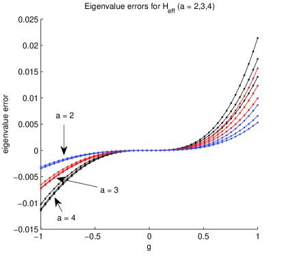
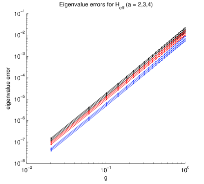
Figure 2: (Color online) Left: Error in the 3 lowest eigenvalues using $\hat{V}_{\mathrm{eff}}^{(a)}$, $a=2$ (black), $a=3$ (red), and $a=4$ (blue) compared to exact eigenvalues ($A=5$). Right: logarithmic plot for $g>0$, showing almost perfect $g^{3}$-behavior.

By investigating the remaining eigenvalues, we confirm that all effective eigenvalues behave in the described way, with only small variations.

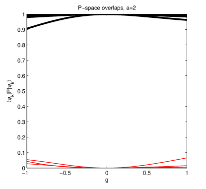
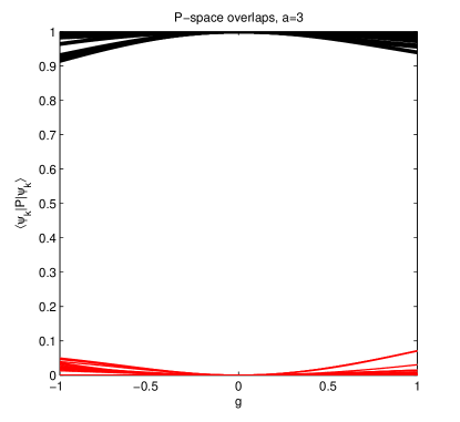
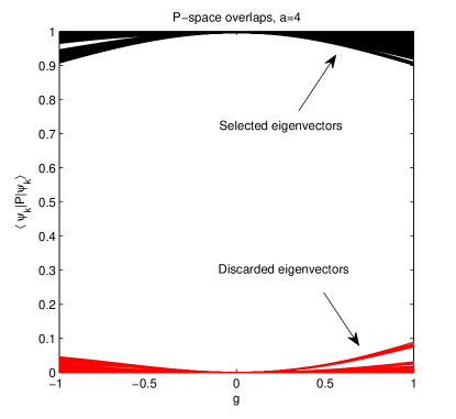
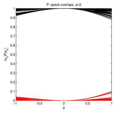
Figure 3: (Color online) Model space overlaps for $a\leq 5$, $f=0$. Black lines are selected model space vectors’ overlaps $\langle\psi_{k}|P|\psi_{k}\rangle$, while red lines are excluded space overlaps. Each line corresponds to one eigenvector of the $a$-body Hamiltonian. The $\mathcal{P}$-space selections and $\mathcal{Q}$-space selections are clearly separated from each other.

To assess the quality of the overlap selection scheme in this case, we graph the overlaps $\langle\psi_{k}|P|\psi_{k}\rangle$ of the selected and discarded eigenvectors for each $a\leq 5$ as a function of $g$ in Fig. 3. Here, the selected overlaps are shown in black, while the discarded are colored red. We show only overlaps in the total spin $S=0$ ($a=2,4$) and $S=1/2$ ($a=3,5$) channels for clarity. The selections for the $\mathcal{P}$-space and the $\mathcal{Q}$-space are well separated for all $g$, meaning that the selection scheme manages to follow the eigenpairs adiabatically from $g=0$, where $\langle\psi_{k}|P|\psi_{k}\rangle$ is either zero or unity. Moreover, the view of the $\mathcal{P}$-space as being “effective” is sensible. However, for very large values of $g$, the graphs of the selected and discarded eigenvectors cross, meaning that the effective interaction view is broken.

We conclude that the effective interaction $\hat{V}_{\mathrm{eff}}^{(a)}$ works very well in the pure pairing Hamiltonian case, as long as the strength $g$ is sufficiently small. However, there is not much to gain with respect to accuracy by going to $a>2$ compared to $a=2$. That is, a two-body effective interaction captures the relevant physics when only a pairing force is involved. In nuclear physics, the pairing interaction is rather strong, and the typical relation between the single-particle spacing $\xi$ around the Fermi surface and the strength of the nuclear pairing interaction $g$ is roughly $|\xi/g|\sim 1-5$. In light nuclei like ¹⁶O, the shell-gap is $11.25$ MeV, and the average $p$-shell and $sd$-shell effective interactions are of the order of $1-5$ MeV in absolute value [30]. In the region of the rare earth nuclei, typical single-particle spacings are of the order of some few hundred keV. The interaction matrix elements are of the same size in absolute value. Choosing thereby a parameter $g$ slightly larger or smaller than one captures the essential physics produced by a pairing interaction around the Fermi surface in nuclei.

2.4 Pairing and particle-hole interaction

We now turn on the particle-hole interaction, by setting $f=\alpha g$ with $\alpha>0$. In this case, the qualitative picture of the model space overlaps shown in Fig. 3 changes dramatically, even for very small values of $\alpha$. In Fig. 4, we repeat the plots from Fig. 3 for $a\leq 4$ with $\alpha=0.05$. It is hard to see any systematic behaviour except for the $a=2$ case. This goes to show that even tiny changes in an operator can give big changes in qualitative behaviour of its eigenvectors, even though the eigenvalues are only perturbed slightly.

In the lower right plot of Fig. 4, we have singled out the overlaps belonging to the lowest eigenvalues for $a=3$. It shows that there is still some ability left in the overlap selection scheme to select some eigenvalues adiabatically. The fifth overlap curve (and all the others not shown) has discontinuities, which would manifest itself as discontinuities in $\hat{V}_{\mathrm{eff}}^{(3)}$.

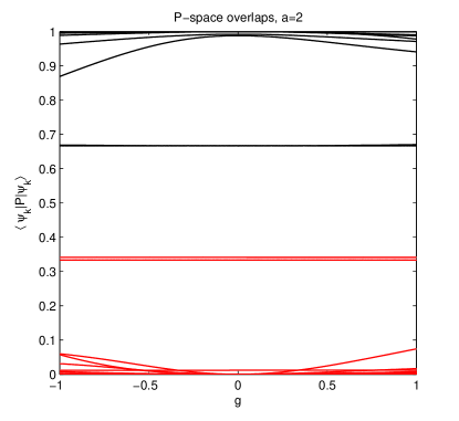
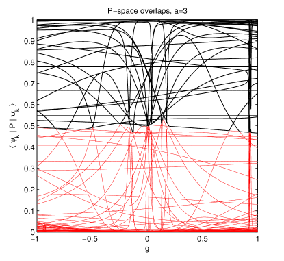
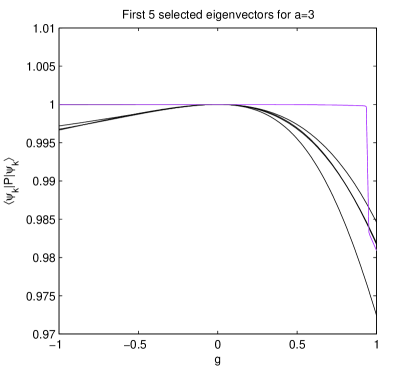
Figure 4: (Color online) Model space overlaps for $a=2,3$, $\alpha=0.05$. Top figures: Black lines are selected model space overlaps, while red lines are excluded space overlaps. The $\alpha=0$ picture (cf. top row of Fig. 3) is radically changed. For $a=4$ (not shown) the picture is even more complicated. These graphs show that it is difficult to choose a proper model space when the particle-hole interaction is turned on. Bottom figure: Singling out the five first selected overlaps for $a=3$; the fifth (purple) shows a discontinuity. Note the vertical scale of the graphs. This shows that some of the chosen eigenpairs (typically the lowest) are chosen correctly.

This trend is general, as Table 1 shows. Here, the fraction $d/m$ of the number of continuous overlaps $d$ (counted visually) over model space dimension $m$ for different $a$ and $\alpha$ are shown for the subspace of lowest $S=0$ or $S=1/2$ (for $a=3$). Apparently, $a>2$ gives a smaller fraction of continuous curves, meaning that following the eigenvalues adiabatically becomes increasingly difficult. The fact that the two-body case exhibits such good behavior is mainly due to the role played by the pairing force if the pairing force is stronger than the particle-hole contribution. With three or more active particles, our choice of particle-hole operator produces strong correlations between the model space and the excluded space.

Table 1: Fraction $d/m$ of “good” selections of eigenpairs for $\hat{V}_{\mathrm{eff}}^{(a)}$, where $m$ is the dimension of $\mathcal{P}$. We limit the attention to states with quantum numbers $S=0=S_{z}=0$ for $a=2$,$4$, and $S=1/2=S_{z}=1/2$ for $a=3$. Also, $f=0.5g$. The $a=2$ case has a much larger fraction than the others, i.e., the overlap selection scheme works better.

	$a=2$	$a=3$	$a=4$
$g=0.05$	$15/15$	$4/40$	$9/50$
$g=0.1$	$15/15$	$4/40$	$9/50$
$g=0.5$	$11/15$	$4/40$	$8/50$
$g=1.0$	$11/15$	$4/40$	$8/50$

These considerations indicate that if any eigenvalues of $\hat{H}_{\mathrm{eff}}^{(a)}$ can be reliable, it will only be the lowest ones. Higher eigenvalues will almost certainly be without meaning. Of course, the matrix elements due to the “bad” selections (i.e., selections after a discontinuity in the curve) will also affect the lowest eigenvalues, but one can hope that these effects can be neglected. From Table 1 we thus expect $\hat{V}_{\mathrm{eff}}^{(2)}$ to perform better than values of $a$ greater than two, but that only the lowest eigenvalues have a reasonable error behaviour.

In Fig. 5 the eigenvalue error plots of Fig. 2 are repeated, but with $\alpha=0.05$. Clearly, $a=2$ is able to produce sensible results in a wide range of $g$; the other $\hat{V}_{\mathrm{eff}}^{(a)}$ have errors that jump erratically. The picture gets worse when we try $\alpha=0.5$, shown in Fig. 2.4. In this case, not even the $a=2$ case will give reliable results except for perhaps the ground state energy. We mention that in Fig. 4 the $a=2$ overlaps will cross at sufficiently large $\alpha$, explaining thereby the breakdown for the $a=2$ case as well.

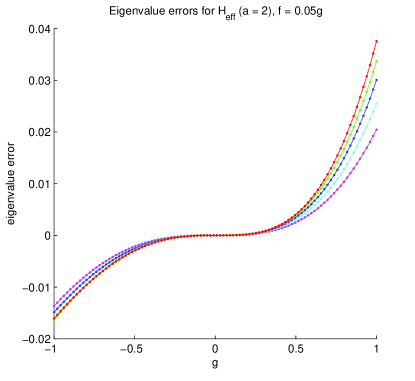
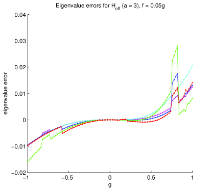
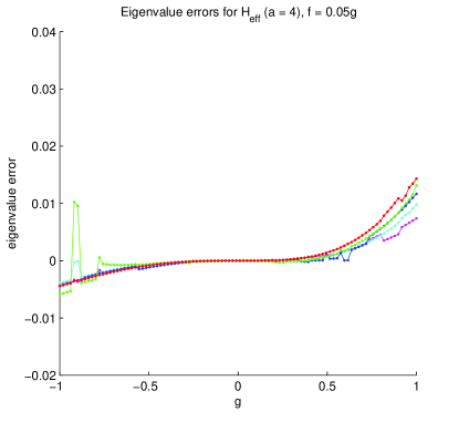
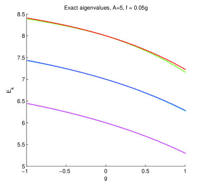
Figure 5: (Color online) A few errors in eigenvalues using $\hat{V}_{\mathrm{eff}}^{(a)}$, $f=0.05g$. Lower right: corresponding exact eigenvalues for $A=5$. Each curve is colored corresponding to the exact eigenvalue curves. The $a=2$ is well-behaved while the $a=3$ case and the $a=4$ case give unreliable eigenvalues.

(Color online) A few errors in eigenvalues using $\hat{V}_{\mathrm{eff}}^{(a)}$, $f=0.5g$. Lower right: corresponding exact eigenvalues for $A=5$. Each curve is colored corresponding to the exact eigenvalue curves. The $a=2$ is now less well behaved. An erratic behaviour is, in all cases, amplified compared to the $f=0.05g$ case. Compare also the error-axis range with Fig. 5.

In summary, the particle-hole interaction changes the qualitative behaviour of the exact eigenvectors for the $a$-body problem drastically. It is clear that it becomes difficult to choose a model space $\mathcal{P}$ that fits well with the model space overlaps shown in Fig. 4, such that it becomes possible to follow the eigenvalues adiabatically as a function of $g$. The two-body effective interaction, however, is surprisingly well behaved for a large range of interaction strenghts.

We have seen that using using effective interactions with $a>2$ does not seem to yield extra accuracy in general compared to the $a=2$ case. First of all, such $\hat{V}_{\mathrm{eff}}^{(a)}$ interactions are much harder to compute. Secondly, we have observed only a constant factor gain in accuracy in the pairing case, in addition to obvious problems when the particle-hole interaction is present.

However, with a strong particle-hole interaction, intruder-states can start playing a major role, and effective many-body interactions with $a>2$ are not capable of reproducing the low-lying levels. The crossings of the curves in, for example, Fig. 4 are due to intruder states, and these are totally absent in integrable systems in contrast to the apparent abundance seen here. Indeed, all two-particle systems described by central force interactions and external harmonic oscillator potentials are classically integrable. There are several examples of nuclear systems where intruder states play a major role, with perhaps the so-called island of inversion for nuclei with mass number $A\sim 31-33$ as one of the more popular mass regions studied recently (see for example the experimental results on the $\beta$-decay of ³³Mg in Ref. [31]). Both the parent and the daughter (³³Al) nuclei reveal intruder-state configurations of two-particle-two-hole character in the lowest excited states, in addition to proposed admixtures of one-particle-one-hole and three-particle-three-hole configurations for the ground state of ³³Mg.

From our results, we may therefore infer that when intruder states are present, special attention must be paid to the construction of an effective interaction, as pointed out almost four decades ago by Schucan and Weidenmüller [27, 28].

To link this discussion with the topic of missing many-body correlations, we can view the presence of intruder states as an example of a model space which is too small. This is in turn reflected in missing many-body correlations beyond those which can be produced by say a given sub-cluster effective interaction. Reducing the model space thus produces missing many-body correlations, which, depending on the strength of the interaction, can produce large differences between the exact results and those obtained with a sub-cluster effective interaction.

We can therefore summarize by saying that an effective sub-cluster Hamiltonian will always produce missing many-body physics. The size of these contributions can normally only be determined a posteriori, that is after a calculation has been performed. To be able to estimate the role of these effects is important for nuclear many-body theory, as it provides us with a sound error estimate. The hope is obviously that their effect is negligible, although the calculations of Ref. [32] indicate small but non-negligible four-body contributions for ⁴He when a three-body Hamiltonian that reproduces the experimental binding energy of ³H is employed. When one employs nuclear forces derived from effective field theory, many-body terms such as three-body interaction arise naturally [2]. There are now clear indications from several calculations (see for example Refs. [3, 8, 9, 32, 33, 34, 35, 36]) that at least three-body interactions have to be included in nuclear many-body calculations. Whether four-body, or more complicated many-body, interactions are important or not for an accurate description of nuclear data is an open issue. From a practical and computational point of view, we obviously favour negligible four or higher many-body interactions.

To understand how many-body interactions develop as one adds more and more particles is thus an open and unsettled problem in nuclear many-body physics (or many-body physics in general if the effective Hilbert space is too small). These interactions are not observables; however, their role can be extracted from calculations with a given effective sub-cluster interaction.

To make this clear, assume that a given three-body Hamiltonian derived from effective field theory has been used to study the chain of oxygen isotopes. With this Hamiltonian, we perform then precise many-body calculations for all isotopes from ¹⁶O to ²⁸O. If the errors of our calculations are negligible, we can infer that these are the results with this specific effective Hamiltonian. The discrepancy between theory and experiment can then be used to extract the role of missing many-body forces as a function of the number of nucleons. The missing many-body physics depends obviously on the employed effective Hamiltonian.

Experiment or simple models provide us therefore with the benchmark our favourite theory has to reproduce. If the experimental data are reproduced to within given uncertainties, one can start analyzing the properties of nuclei in terms of various components of the nuclear forces. This can allow for the extraction of simple physical mechanisms, as done recently by Otsuka et al [37].

This coupling between experiment and precise many-body calculations is what we will sketch in the next section, starting with the oxygen isotopes.

3 Physics cases

The nuclear forces derived from effective field theory are obviously much more complicated than the above simple model. First of all, our simple model contains only a two-body Hamiltonian. It allowed for a numerically exact diagonalization for a five-particle system in a Hilbert space consisting of eight doubly degenerate single-particle states. An effective sub-cluster interaction defined for a smaller space (typically the five lowest doubly degenerate single-particle states) gave results which were close to the exact ones if the interaction was weak and a relevant model space was employed. In particular, with a particle-hole interaction, one can easily get a strong admixture from states outside the chosen model space. In that case, the various sub-cluster effective interactions failed in reproducing the low-lying eigenvalues.

The nuclear interactions derived from effective field theories [2] already contain at the so-called N²LO level, three-body interactions. At the N³LO level, four-body interactions appear. These interactions are normally constructed for a given cutoff $\Lambda$. In principle, if one uses an interaction at the N³LO level, one should also include four-body interactions. Normally, only three-body interactions at the N²LO level are introduced, together with a two-body interaction that fits two-particle data (scattering data and bound state properties) at the N³LO level.

This means that when employed in a many-body context with more than three particles, our Hamiltonian lacks some many-body correlations. Hopefully these are small. A comparison with data, if our theory produces converged results at a given level of many-body physics, may then reveal their importance.

In this sense, a given nuclear interaction computed with effective field theory at a given NⁿLO level, should contain all possible many-body interactions. At the N³LO level, one should include one-body, two-body, three-body, and four-body interactions. Omitting some of these leads to a sub-cluster effective Hamiltonian. In a certain sense, this parallels the discussion from the previous section. However, in the nuclear physics case, it is important to keep in mind that these interactions have been derived with a specific energy cutoff. The energy cutoff defines our effective Hilbert space, or model space. If the model space defined for an actual many-body calculation does not include all possible excitations within this model space, one can easily end up with the type of missing many-body correlations discussed in the previous section.

To make our scheme more explicit, assume that we are planning a calculation of the oxygen isotopes with an effective field theory interaction that employs a cutoff $\Lambda=600$ MeV. Assume also that our favourite single-particle basis is the harmonic oscillator, with single-particle energies $\varepsilon_{nl}=\hbar\omega(2n+l+3/2)$, with $\omega$ the oscillator frequency, $n=0,1,2,\dots$ being the number of nodes and $l$ the single-particle orbital momentum. The oscillator length $b$ is defined as

$$b=\sqrt{\frac{\hbar}{m\omega}}.$$

We define $p=0,1,2,\dots,P$ with $P=2n+l$ as the quantum number $p$ of the highest-filled level. The level labelled $p$ can accommodate $(p+1)(p+2)$ fermions, with a spin degeneracy of two for every single-particle state taken into account. For a given maximum value of $P=2n_{\mathrm{max}}+l_{\mathrm{max}}$, we have a total of

$$N=\sum_{p=0}^{P}(p+1)(p+2)=\frac{(P+1)(P+2)(P+3)}{3},$$

single-particle states.

The cutoff $\Lambda$ defines the maximum excitation energy a system of $A$ nucleons can have. The largest single-particle excitation energy (corresponding to possible one-particle-one-hole correlations) is then

$$\Lambda=\hbar\omega P=\hbar\omega(2n_{\mathrm{max}}+l_{\mathrm{max}}).$$

The value of $\hbar\omega$ can be extracted from the mean-squared radius of a given nucleus. One can show that this results in [38]

$$\hbar\omega\approx\left(\frac{3}{2}\right)^{4/3}\frac{\hbar^{2}}{2m_{N}r_{0}^{2}}A^{-1/3},$$

with $r_{0}\approx 1$ fm. Setting $A=16$ and $\Lambda=600$ MeV results in $P\approx 42$. The largest possible value for $n$ is then $n_{\mathrm{max}}\approx 21$, or 22 major shells. With $P=42$, the total number of single-particle states in this model space is $28380$!

For ¹⁶O, this means that we have to distribute eight protons and eight neutrons in $28380$ single-particle states, respectively. The total number of Slater determinants, with no restrictions on energy excitations, is

$$\left(\begin{array}[]{c}28380\\ 8\end{array}\right)\times\left(\begin{array}[]{c}28380\\ 8\end{array}\right)\approx 10^{62}.$$

Any direct diagonalization method in such a huge basis is simply impossible. One possible approach is to introduce a smaller model space with a pertinent effective interaction, similar to what was discussed in the previous section. Depending on the size of the model space and the strength of the interaction, this can lead to uncontrolled many-body correlations, with effects similar to what was discussed within the framework of the simple model from Section 2. This has been the philosophy of the no-core shell-model approach [8] or many-body perturbation theory [16]. Another alternative is to employ methods which allow for systematic inclusions to all orders of specific sub-clusters of correlations within the full model space defined by $\Lambda$. This reduces the computational effort considerably and accounts, at the same time, for most of the relevant degrees of freedom. The Coupled cluster method [15, 39, 40] and Green’s function theory [10] allow for such systematic expansions starting from a given Hamiltonian.

Coupled-cluster theory has been particularly successful in both quantum chemistry and nuclear physics. It fulfills basically all the requirements we listed in Section 1. Furthermore, with a given truncated single-particle basis (our effective Hilbert space) we can extract precise error estimates on the energy [14, 41]. It is a topic of current research to be able to predict and understand the error due to truncations in the number of many-body correlations. As an example, most coupled-cluster calculations seldom go beyond correlations of the three-particle-three-hole type, the so-called triples correlations. An estimate of the error made due to the omission of four-particle-four-hole correlations (and higher-order correlations) would therefore be very useful. That would lead to a much more predictive theory.

3.1 Brief review of coupled cluster theory

Our many-body method of choice is thus coupled-cluster theory, see Refs. [15, 39, 40] for more details. The coupled-cluster method fulfills Goldstone’s linked-cluster theorem and therefore yields size-extensive results, i.e., the error due to the truncation is linear in the mass number $A$ of the nucleus under consideration. Size extensivity is an important issue when approximate solutions to all but the lightest nuclei are sought [15, 42]. Second, the computational effort scales gently (i.e., polynomial) with increasing dimension of the single-particle basis and the mass number $A$. The method has met benchmarks in light nuclei [33, 43].

Our algorithm is as follows:

1. We start with a nuclear force from effective field theory at a given NⁿLO order. In the calculations we present here, we include only a nucleon-nucleon interaction to order N³LO. We neglect three-nucleon forces since their application within the coupled-cluster method is still limited to smaller model spaces [34]. This gives rise to one source of systematic error and most likely the largest uncertainty in our results. So-called power-counting estimates from chiral effective field theory result in an uncertainty of about 2 MeV per nucleon, see Ref. [9] for further details.

2. We compute ground state properties and excited states by including one-particle-one-hole, two-particle-two-hole, and selected three-particle-three-hole correlations. These correlations are called singles, doubles, and triples, respectively. We consider corrections due to triples excitations within the so-called $\Lambda$CCSD(T) approximation, see for example [9] for more details. Comparison of a calculation which includes only one-particle-one-hole and two-particle-two-hole correlations (CCSD), see Ref. [9], shows that triples corrections account for 10-15%. Similar ratios are found in coupled-cluster calculations of atoms and molecules, and experience in quantum chemistry (see for example Ref. [15]) suggests that the truncation of the cluster amplitudes beyond the triples corrections introduces an error of a few percent.

3. The actual single-particle space used is defined close to the effective field theory model space. Our error here is smaller than the error made in the previous two points. The final results are more or less converged as a function of the size of the model space. A precise error estimate for a given single-particle basis was presented within a configuration interaction approach by Kvaal [14]. Similar error estimates apply to coupled-cluster theory as well [41].

Within the choice of model space, most of our expectation values are practically converged. This is, for example, reflected in the fact that the ground state energy is almost independent of the chosen harmonic oscillator energy (for demonstrations, see for example Refs. [9, 33, 40]). From this, we can infer that our specific many-body approximation yields probably the optimal result which can be achieved at this specific level of many-body physics. Eventual discrepancies with experiment can then most likely be attributed to missing many-body correlations. A typical case would be the lack of three-body interactions from effective field theory.

3.2 Oxygen isotopes

The oxygen isotopes are the heaviest isotopes for which the drip line is well established. There are large experimental campaigns worldwide [44, 45, 46] which aim at uncovering the properties of the oxygen isotopes, both at or close to the drip line and beyond. Two out of four stable even-even isotopes exhibit a doubly magic nature, namely ²²O ($Z$=$8$,$N$=$14$) [47] and ²⁴O ($Z$=$8$, $N$=$16$) [48, 49]. The structure of these two doubly magic nuclei is assumed to be governed by the evolution of the $1s_{1/2}$ and $0d_{5/2}$ one-quasiparticle states. The isotopes ^25-28O are all believed to be unstable towards neutron emission, even though ²⁸O is a doubly magic nucleus within the standard shell-model picture.

Of interest to us is the fact that we can perform ab initio coupled-cluster calculations for all assumed closed-shell nuclei of this isotopic chain, that is, oxygen isotopes with $A=16$, $A=22$, $A=24$, and $A=28$. Furthermore, we can also compute the $A\pm 1$ nuclei such as ²⁵F, ²⁵O, and ²³N. This means further that we can extract the isospin dependence of say spin-orbit partners. In Ref. [9] we considered the nuclei ^16,22,24,28O and computed their ground-state energies within the $\Lambda$CCSD(T) approximation for chiral interactions with cutoffs of $\Lambda_{\chi}=500$ MeV and $\Lambda_{\chi}=600$ MeV, respectively. Figure 6 shows the ground state energies relative to ²²O.

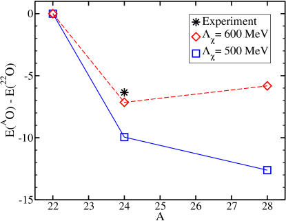
Figure 6: (Color online) Ground-state energies of neutron-rich oxygen isotopes ^AO relative to ²²O for chiral interactions with two different cutoffs $\Lambda_{\chi}$. Taken from Ref. [9].

At a cutoff $\Lambda_{\chi}=500$ MeV, we find that ²⁸O is bound by about 2.7 MeV with respect to ²⁴O. However, the situation is reversed at the higher cutoff $\Lambda_{\chi}=600$ MeV, and the difference is about -1.3 MeV. With the uncertainties due to missing three-body interactions, it is presently not possible to reach a conclusion regarding the existence of ²⁸O. However, using interactions from chiral effective field theory, we see that the stability of ²⁸O depends mainly on the contributions of the three-nucleon force (and probably more complicated many-body forces), and that even small contributions can tip the balance in either direction. A mass measurement of ²⁸O is clearly needed.

The above results show that we do not yet understand fully how many-body forces evolve as we add more nucleons. The hope is that the inclusion of a three-body interaction from effective field theory reduces the dependence on the cutoff at the two-body level. This was nicely demonstrated by Jurgenson et al [32] in a recent study of ³H and ⁴He. For ⁴He, there were indications that a small four-body interaction may be needed, as also demonstrated by Epelbaum et al [3]. Our ab initio calculations indicate also that the recent results from phenomenological shell-model approaches regarding the unbound character of ²⁸O should be viewed with caution. The combination of three-nucleon forces, the proximity of the continuum, and the isospin dependence are a challenge for reliable theoretical predictions, see also Refs. [50, 51].

Summarizing, we can claim that there is a posteriori evidence of the need of a three-body interaction or more complicated interactions. We hope that with the inclusion of three-body forces, the difference seen for different chiral interactions should become small.

Furthermore, if the differences between theory and experiment are small, theory can be used to extract simple information on say various components of the nuclear force. We can, for example, study the evolution of many-body forces as we increase the number of valence nucleons. One possibility is to extract the $A$-dependence and the isospin dependence of such correlations as we move towards the drip line. Another interesting quantity which can be extracted is the isospin and $A$-dependence of the spin-orbit force. This will allow us to answer and understand which mechanisms change the single-particle fields close to the drip line. For these mass regions and the oxygen isotopes, experimental data on ²⁸O are very important. Similarly, for spin-orbit partners, measurements of closed-shell nuclei with one particle added or removed beyond $A=24$ will allow us to benchmark theory with experiment and perhaps understand which parts of the nuclear force are important close to the drip line.

3.3 Calcium and nickel isotopes

Doubly magic nuclei are particularly important and closed-shell nuclei like ⁵⁶Ni, ¹⁰⁰Sn and ¹³²Sn have been the focus of several experiments during the last several years [52, 53, 54, 55, 56, 57, 58, 59, 60]. Their structure provides important information on theoretical interpretations and our basic understanding of matter. In particular, recent experiments [52, 53, 54, 55, 56, 57] have aimed at extracting information about single-particle degrees of freedom in the vicinity of ⁵⁶Ni. Experimental information from single-nucleon transfer reactions and magnetic moments [52, 53, 54, 55, 57] can be used to extract and interpret complicated many-body wave functions in terms of effective single-particle degrees of freedom. Transfer reactions provide, for example, information about the angular distributions, the excitation energies, and the spectroscopic factors of possible single-particles states.

Much of the philosophy exposed in the previous subsection can be repeated for studies of calcium and nickel isotopes. The interesting feature here is that we probe systems with more nucleons. The chain of nickel isotopes exhibits four possible closed-shell nuclei, namely ⁴⁸Ni, ⁵⁶Ni, ⁶⁸Ni, and ⁷⁸Ni, with a difference of 30 neutrons from ⁴⁸Ni to ⁷⁸Ni. Similarly, for calcium isotopes in the $fp$-shell, we have 20 neutrons that can be added to ⁴⁰Ca and five possible closed-shell nuclei, ⁴⁰Ca, ⁴⁸Ca, ⁵²Ca, ⁵⁴Ca and ⁶⁰Ca. The binding energies of ⁵⁴Ca and ⁶⁰Ca are presently not available. Moreover, compared with the oxygen isotopes with at most 12 nucleons in the $sd$-shell outside ¹⁶O, different single-particle degrees of freedom are probed. Comparing theory and experiment can again provide important information about spin-orbit partners close to the drip line, with information on their density and isospin dependence as well.

As stated in the previous subsection, we are in the position where such nuclei can be calculated rather accurately with a given two-body Hamiltonian. This is demonstrated in Refs. [10, 40]. We are not limited to closed-shell systems but can also compute ground states and excited states of $A\pm 1$ ($A$ is the closed-shell nucleus) nucleons rather precisely. It means that a nucleus like ⁷⁹Cu can be accessed with ab initio methods like coupled cluster theory. Single-particle properties like magnetic moments and spectroscopic factors can then give a measure of how good a closed nucleus ⁷⁸Ni is. Experimental data which probe single-particle properties on $A\pm 1$ systems close to the dripline, will therefore provide important benchmarks for theory.

3.4 Ab initio studies of nuclei around mass $A=100$

We end this section by stating that the analysis which can be performed for $fp$-shell and $sd$-shell nuclei can be extended to the region of the tin isotopes as well, with both ¹⁰⁰Sn and ¹³²Sn as two very important nuclei for our understanding of the stability of matter, see for example the recent works of Refs. [58, 59, 60, 61]. In this case we expect to be able to run similar calculations within the next two to three years for nuclei like ¹⁰⁰Sn, ¹³²Sn, and ¹⁴⁰Sn together with the corresponding $A\pm 1$ nuclei. We can then test the development of many-body forces for an even larger chain of isotopes and provide theoretical benchmarks for nuclei near ¹⁴⁰Sn, of great importance for the understanding of the $r$-process, a nucleosynthetic process responsible for the production of around half of the heavy elements. A recent experiment on ¹³²Sn shows clear evidence that this nucleus is an extremely good closed-shell nucleus [61]. This has, in turn, consequences for our understanding of quasi-particle properties in this mass region. We mention also here that ¹³⁷Sn is the last reported neutron-rich isotope (with half-life). Our final aim is to provide reliable predictions for all possibly closed-shell nuclei, from $A=4$ to $A=208$.

4 Conclusions

The aim of this article has been to shed light on our understanding of many-body correlations in nuclei. Since all theoretical calculations involve effective Hamiltonians and effective Hilbert spaces, it is crucial to have a handle on the role many-body correlations play in a many-body system. This means that a sound theory should provide error estimates on the importance of neglected many-body effects. To understand these and develop sound error estimates is mandatory if one wants to have a predictive theory.

We are now in a position where fairly precise results can be obtained for several closed-shell nuclei with a given two-body Hamiltonian. However, since most two-body interactions used nowadays are based on chiral effective field theory, it means that three-body and, more complicated, many-body interactions arise at different chiral orders [2]. The neglect of such higher-order terms leads to different predictions for two-body Hamiltonians. Experiment can then be used to understand how important these neglected degrees of freedom are. Stated in a more philosophical way, we seem to be doing pretty well at ‘doing the problem right’ (verification); but we still struggle with ‘validation’ (doing the right problem). Having now developed the tool set to rigorously solve the nuclear many-body problem accurately, we can use these tools to more fully investigate the nuclear interaction.

The hope is that the addition of three-body interactions will produce results which are more or less independent of the cutoff used in chiral effective field theory. This means, in turn that if our theoretical calculations with a three-body Hamiltonian reproduce, for example, experimental binding energies to high accuracy (theoretical and compared with experiment), we can then start analyzing properties like single-particle energies close to the drip line or the $A$-dependence of missing many-body correlations. Our formalism allows us now to compute closed-shell nuclei along an isotopic chain and extract single-particle energies and properties. For the chains of oxygen, calcium, nickel, and tin isotopes, we can therefore provide important information about nuclear structure at the drip lines of these chains. But in order to do this, one needs experimental data on properties like the binding energies of ²⁸O or ⁵⁴Ca. We feel that the enormous progress which has taken place in the last few years in nuclear theory can really lead to a predictive and reliable approach to nuclear many-body systems. In this endeavor, the close ties between theory and experiment are crucial in order to understand properly the limits of stability of matter.

References

References

- [1] B. R. Barrett, D. J. Dean, M. Hjorth-Jensen, and J. P. Vary, J. Phys. G 31, 1 (2005).
- [2] E. Epelbaum, H.-W. Hammer, and U.-G. Meißner, Rev. Mod. Phys. 81, 1773 (2009).
- [3] E. Epelbaum, H. Krebs, D. Lee, and U.-G. Meißner, arXiv:0912.4195.
- [4] N. Ishii, S. Aoki, and T. Hatsuda, Phys. Rev. Lett. 99, 022001 (2007).
- [5] S. Aoki, T. Hatsuda, and N Ishii, Comput. Sci. Disc. 1, 015009 (2008).
- [6] S. R. Beane, W. Detmold, Huey-Wen Lin, T. C. Luu, K. Orginos, M. J. Savage, A. Torok, and A. Walker-Loud, arXiv:0912.4243.
- [7] S. K. Bogner, R. J. Furnstahl, and A. Schwenk, arXiv:0912.3688
- [8] P. Navratil, S. Quaglioni, I. Stetcu, and B. R. Barrett, J. Phys. G 36, 08310 (2009).
- [9] G. Hagen, T. Papenbrock, D. J. Dean, M. Hjorth-Jensen, and B. Velamur Asokan, Phys. Rev. C 80, 021306 (2009).
- [10] C. Barbieri, Phys. Rev. Lett. 103, 202502 (2009); C. Barbieri and M. Hjorth-Jensen, Phys. Rev. C 79, 064313 (2009).
- [11] J. Dobaczewski, B. G. Carlsson, and M. Kortelainen, arXiv:1002.3646
- [12] B. Gebremariam, T. Duguet, and S. K. Bogner, arXiv:0910.4979.
- [13] J. E. Drut, R. J. Furnstahl, and L. Platter, Prog. Part. Nucl. Phys. 64, 120 (2010).
- [14] S. Kvaal, Phys. Rev. B 80, 045321 (2009).
- [15] R. J. Bartlett and M. Musial, Rev. Mod. Phys. 79, 291 (2007).
- [16] M. Hjorth-Jensen, T. T. S. Kuo, and E. Osnes, Phys. Rep. 261, 125 (1995).
- [17] J. H. Van Vleck, Phys. Rev. 33, 467 (1929).
- [18] C. Bloch, Nucl. Phys. 6, 329 (1958).
- [19] J. Bloch and C. Horowitz, Nucl. Phys. 8, 91 (1958).
- [20] B. H. Brandow, Rev. Mod. Phys. 39, 771 (1967).
- [21] B. H. Brandow, Adv. Quantum Chem. 10, 187 (1977).
- [22] B. H. Brandow, Int. J. Quant. Chem. 15, 207 (1979).
- [23] D. J. Klein, J. Chem. Phys. 61, 786 (1974).
- [24] I. Shavitt and L. T. Redmon, J. Chem. Phys. 73, 5711 (1980).
- [25] S. Kvaal, Phys. Rev. C 78, 044330 (2008).
- [26] K. Suzuki, Prog. Theor. Phys. 68, 1627 (1982); S.Y. Lee and K. Suzuki, Phys. Lett. B 91, 79 (1980); K. Suzuki and S.Y. Lee, Prog. Theor. Phys. 64, 2091 (1980).
- [27] T. H. Schucan and H. A. Weidenmüller, Ann. Phys. (N.Y.) 73, 108 (1972).
- [28] T. H. Schucan and H. A. Weidenmüller, Ann. Phys. (N.Y.) 76, 483 (1973).
- [29] P. A. Schaefer, Ann. Phys. (N.Y.) 87, 375 (1974).
- [30] S. Kvaal and M. Hjorth-Jensen, unpublished.
- [31] V. Tripathi, S. L. Tabor, P. F. Mantica, Y. Utsuno, P. Bender, J. Cook, C. R. Hoffman, Sangjin Lee, T. Otsuka, J. Pereira, M. Perry, K. Pepper, J. S. Pinter, J. Stoker, A. Volya, and D. Weisshaar, Phys. Rev. Lett. 101, 142504 (2008).
- [32] E. D. Jurgenson, P. Navratil, and R. J. Furnstahl, Phys. Rev. Lett. 103, 082501 (2009).
- [33] G. Hagen, D. J Dean, M. Hjorth-Jensen, T. Papenbrock, and A. Schwenk, Phys. Rev. C76, 044305 (2007).
- [34] G. Hagen, T. Papenbrock, D. J Dean, A. Schwenk, A. Nogga, M. Wloch and P. Piecuch, Phys. Rev. C76, 034302 (2007).
- [35] Steven C. Pieper, V. R. Pandharipande, R. B. Wiringa, and J. Carlson, Phys. Rev. C 64, 014001 (2001).
- [36] R. B. Wiringa and Steven C. Pieper, Phys. Rev. Lett. 89, 182501 (2002).
- [37] T. Otsuka, T. Suzuki, M. Honma, Y. Utsuno, N. Tsunoda, K. Tsukiyama, and M. Hjorth-Jensen, Phys. Rev. Lett. 104, 012501 (2010).
- [38] M. W. Kirson, Nucl. Phys. A 781, 350 (2007).
- [39] D. J. Dean and M. Hjorth-Jensen, Phys. Rev. C 69, 54320 (2004).
- [40] G. Hagen, T. Papenbrock, D. J. Dean, and M. Hjorth-Jensen, Phys. Rev. Lett. 101, 092502 (2008).
- [41] R. Schneider, Numer. Math. 113, 433 (2009).
- [42] D. J. Dean, G. Hagen, M. Hjorth-Jensen, T. Papenbrock, and A. Schwenk, Phys. Rev. Lett. 101, 119201 (2008).
- [43] B. Mihaila and J.H. Heisenberg, Phys. Rev. C 61, 054309 (2000); Phys. Rev. Lett. 84, 1403 (2000).
- [44] Z. Elekes et al, Phys. Rev. Lett. 98, 102502 (2007).
- [45] A. Schiller et al, Phys. Rev. Lett. 98, 102502 (2007).
- [46] C. R. Hoffman et al, Phys. Rev. Lett. 100, 152502 (2008).
- [47] P. G. Thirolf et al, Phys. Lett. B485, 16 (2000).
- [48] M. Stanoiu et al, Phys. Rev. C 69, 034312 (2004).
- [49] C. R. Hoffman et al, Phys. Lett. B672, 17 (2009).
- [50] T. Otsuka, T. Suzuki, J. D. Holt, A. Schwenk, and Y. Akaishi, arXiv:0908.2607.
- [51] K. Tsukiyama, M. Hjorth-Jensen, and G. Hagen, Phys. Rev. C 80, 051301 (2009).
- [52] K. L. Yurkewicz et al, Phys. Rev. C 70, 064321 (2004).
- [53] K. L. Yurkewicz et al., Phys. Rev. C 74, 024304 (2006).
- [54] J. Lee, M. B. Tsang, W. G. Lynch, M. Horoi, and S. C. Su, preprint ArXiv:0809.4686; M. B. Tsang et al, preprint ArXiv:0810.1925 and National Superconducting Cyclotron Laboratory, Michigan State University, proposal 06035.
- [55] A. Gade et al, unpublished and National Superconducting Cyclotron Laboratory, Michigan State University, proposal 06020.
- [56] G. Kraus et al, Phys. Rev. Lett. 73, 1773 (1994).
- [57] K. Minamisono et al, Phys. Rev. Lett. 96, 102501 (2006).
- [58] D. Bazin et al, Phys. Rev. Lett. 101, 252501 (2008).
- [59] D. Seweryniak et al, Phys. Rev. Lett. 101, 252501 (2008).
- [60] I. Darby et al, unpublished (2010), submitted to Nature.
- [61] K. Jones et al, unpublished (2010), submitted to Nature.