Trace Formulae and Spectral Statistics for Discrete Laplacians on Regular Graphs ($\@slowromancap ii@$)

Abstract

Following the derivation of the trace formulae in the first paper in this series, we establish here a connection between the spectral statistics of random regular graphs and the predictions of Random Matrix Theory (RMT). This follows from the known Poisson distribution of cycle counts in regular graphs, in the limit that the cycle periods are kept constant and the number of vertices increases indefinitely. The result is analogous to the so called “diagonal approximation” in Quantum Chaos. We also show that by assuming that the spectral correlations are given by RMT to all orders, we can compute the leading deviations from the Poisson distribution for cycle counts. We provide numerical evidence which supports this conjecture.

1 Introduction

The present paper is the second in this series, where we aim to establish a rigorous connection between the spectral fluctuations in the spectra of random regular graphs and the predictions of Random Matrix Theory (RMT). In the first paper [1] (to be referred to as $\@slowromancap i@$) we provided the necessary definitions and facts about graphs and we shall use the same notations here. Suffice it to say that we deal with the ensemble $\mathcal{G}_{V,d}$ of $d$-regular graphs on $V$ vertices, and we study the spectrum $\{\mu_{j}\}_{j=1}^{V-1}$ of the adjacency matrix $A$, from which we excluded the trivial eigenvalue $\mu_{V}=d$. The spectral density is defined as

$$\rho^{(A)}(\mu)\equiv\frac{1}{V-1}\sum_{j=1}^{V-1}\delta(\mu-\mu_{j})\ .$$ (1)

In what follows we shall be interested in the large $V$ limit, and in most cases the replacement of $V-1$ by $V$ will be justified. We shall do this consistently to simplify the notation.

In $\@slowromancap i@$ we also defined the ensemble of “magnetic” graphs, $\mathcal{G}^{M}_{V,d}$ where the adjacency matrix of each member of the ensemble $\mathcal{G}_{V,d}$ is decorated by phases

$$M_{i,j}=A_{i,j}{\rm e}^{i\chi_{i,j}}\ \ ;\ \ \chi_{j,i}=-\chi_{i,j}$$ (2)

and the phases are independent random variables distributed uniformly on the unit circle. Here the entire spectrum of $M$ is considered and

$$\rho^{(M)}(\mu)\equiv\frac{1}{V}\sum_{j=1}^{V}\delta(\mu-\mu_{j})\ .$$ (3)

In $\@slowromancap i@$ we prepared the tools needed for our purpose, namely trace formulae. In the sequel, we shall summarize the absolutely necessary information about trace formulae required to make the present paper self contained.

1.1 The trace formula - a short reminder

Trace formulae express the spectral density of the adjacency matrix as a sum of two contributions, $\rho(\mu)\equiv\frac{1}{V}\sum_{j=1}^{V}\delta(\mu-\mu_{j})=\left\langle\rho(\mu)\right\rangle+\tilde{\rho}(\mu)$ where $\left\langle\ \cdot\ \right\rangle$ stands for the ensemble average. Here, For both ensembles, $\left\langle\rho(\mu)\right\rangle$ is the well known Kesten-McKay expression for the mean spectral density [4, 5]

$$\rho_{KM}(\mu)=\lim_{V\rightarrow\infty}\langle\rho(\mu)\rangle=\left\{\begin{array}[]{lcr}\frac{d}{2\pi}\frac{\sqrt{4(d-1)-\mu^{2}}}{d^{2}-\mu^{2}}&\mbox{for}&|\mu|\leq 2\sqrt{d-1}\\ \\ 0&\mbox{for}&|\mu|>2\sqrt{d-1}\end{array}\right.\ .$$ (7)

Note that the Kesten-McKay density depends explicitly on the degree $d$. $\tilde{\rho}(\mu)$ is the fluctuating part of $\rho(\mu)$, with $\left\langle\tilde{\rho}(\mu)\right\rangle=0$. To simplify the notation we omit reference to the $d$ dependence. In the limit $d\gg 1$, $\rho_{KM}$ approaches Wigner’s semi-circle distribution which characterizes the canonical Gaussian random matrix ensembles. The fluctuating parts are expressed as infinite sums over Chebyshev polynomials (of the first kind) $T_{n}(x)$ with coefficients which depend on cycles on the graph. The trace formulae take similar forms for the two ensembles, but with different coefficients.

$$\tilde{\rho}^{(A)}(\mu) = \ \frac{1}{\pi}\sum_{t=3}^{\infty}\frac{y^{(A)}_{t}}{\sqrt{4(d-1)-\mu^{2}}}T_{t}\left(\frac{\mu}{2\sqrt{(d-1)}}\right).$$ (8)

The parameters $y_{t}^{(A)}$ are defined as

$$y^{(A)}_{t}=\frac{1}{V}\frac{Y^{(A)}_{t}-(d-1)^{t}}{(\sqrt{d-1})^{t}}$$ (9)

with $Y^{(A)}_{t}$ the number of $t$-periodic walks where no back scattering is allowed (nb walks). Since $\left\langle Y^{(A)}_{t}\right\rangle=(d-1)^{t}$,  $y^{(A)}_{t}$ is the properly regularized deviation of the number of $t$-periodic nb-walks from their mean. In combinatorial graph theory it is customary to define $C_{t}=\frac{Y^{(A)}_{t}}{2t}$ as the number of $t$-periodic nb cycles. It is known that for $t<\log_{d-1}V$ and asymptotically in $V$, the $C_{t}$ are distributed like independent Poisson variables [6, 7, 8, 9].

The trace formula for the spectral density of magnetic graphs is similar to (8) with the following differences: The entire spectrum of the magnetic adjacency matrix is included in the definition of the spectral density. The coefficients $y^{(M)}_{t}$ are now defined as

$$y^{(M)}_{t}=\frac{1}{V}\frac{Y_{t}^{(M)}}{(\sqrt{(d-1)})^{t}}\ \ ,\ \ Y_{t}^{(M)}=\sum_{\alpha}{\rm e}^{i\chi_{\alpha}},$$ (10)

where the sum above is over all the nb t-periodic walks, and $\chi_{\alpha}$ is the total phase (net magnetic flux) accumulated along the t-periodic walk. For finite $V$, $\left\langle y^{(M)}_{t}\right\rangle\neq 0$ since $\chi_{\alpha}=0$ for nb periodic walks where each bond is traversed equal number of times in the two directions. However, in the limit of large $V$, the number of such walks is small and therefore $\left\langle y^{(M)}_{t}\right\rangle\rightarrow 0$.

1.2 Spectral fluctuations on graphs and RMT- Numerical evidence

So far, the only evidence suggesting a connection between RMT and the spectral statistics on graphs is the numerical studies of Jacobson et. al. [2]. In a preliminary step in the present research, we performed numerical simulations which extended the tests of [2]. While describing these studies, we shall introduce a few concepts from RMT which will be used in the main body of the paper.

It is advantageous to map the spectrum from the real line to the unit circle,

$$\phi_{j}=\arccos\frac{\mu_{j}}{2\sqrt{d-1}}\ \ ;\ \ 0\leq\phi_{j}\leq\pi\ .$$ (11)

This change of variables is allowed since in the limit of large graphs, only a fraction of order $1/V$ of the spectrum is outside the support of the Kesten McKay distribution $[-2\sqrt{d-1},2\sqrt{d-1}]$ [10].

The mean spectral density on the circle is not uniform, and the Kesten McKay density on the circle is

$$\rho_{KM}(\phi)=\frac{2(d-1)}{\pi d}\frac{\sin^{2}\phi}{1-\frac{4(d-1)}{d^{2}}\cos^{2}\phi}\ .$$ (12)

The mean spectral counting function is defined as

$$N_{KM}(\phi)=V\int_{0}^{\phi}\rho_{KM}(\phi)d\phi\ =V\frac{d}{2\pi}\left(\phi-\frac{d-2}{d}\arctan\left(\frac{d}{d-2}\tan\phi\right)\right).$$ (13)

Following the standard methods of spectral statistics, one introduces a new variable $\theta$, which is uniformly distributed on the unit circle. This “unfolding” procedure is explicitly given by

$$\theta_{j}=\frac{2\pi}{V}N_{KM}(\phi_{j})$$ (14)

The nearest spacing distribution defined as

$$P(s)=\lim_{V\rightarrow\infty}\ \frac{1}{V}\left\langle\sum_{j=1}^{V}\delta\left(s-\frac{V}{2\pi}(\theta_{j}-\theta_{j-1})\right)\right\rangle\ ,$$ (15)

is often used to test the agreement with the predictions of RMT (This was also the test conducted in ([2])). In this definition of the nearest spacing distribution, $\theta_{0}$ coincides with $\theta_{V}$, since the phases lie on the unit circle. In figure (1) we show numerical simulations obtained by averaging over 1000 randomly generated $3$-regular graphs on $1000$ vertices and their “magnetic” counterparts, together with the predictions of RMT for the COE and the CUE ensembles [3], respectively. The agreement is quite impressive.

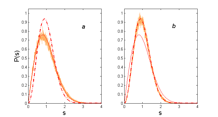
Figure 1: Nearest level spacings for: (a.) Graphs possessing time reversal symmetry. (b.) Magnetic graphs.
Both figures are accompanied with the RMT predictions: Solid line - COE, Dashed line - CUE.

Another quantity which is often used for the same purpose is the spectral form-factor,

$$K_{V}(t)=\frac{1}{V}\left\langle\left|\sum_{j=1}^{V}{\rm e}^{it\theta_{j}}\ \right|^{2}\ \right\rangle\ .$$ (16)

The form-factor is the Fourier transform of the spectral two point correlation function and it plays a very important rôle in the understanding of the relation between RMT and the quantum spectra of classically chaotic systems [3, 13].

In RMT the form factor displays scaling: $\displaystyle\lim_{V\rightarrow\infty}K_{V}(t)=K(\tau\equiv\frac{t}{V})$. The explicit limiting expressions for the COE and CUE ensembles are [3]:

$$K_{COE}(\tau)=\left\{\begin{array}[]{lcr}2\tau-\tau\log{(2\tau+1),}&\mbox{for}&\tau<1\\ \\ 2-\tau\log{\frac{2\tau+1}{2\tau-1},}&\mbox{for}&\tau>1\end{array}\right.\ .$$ (20)

$$K_{CUE}(\tau)=\left\{\begin{array}[]{lcr}\tau,&\mbox{for}&\tau<1\\ \\ 1,&\mbox{for}&\tau>1\end{array}\right.\ .$$ (24)

The numerical data used to compute the nearest neighbor spacing distribution $P(s)$, was used to calculate the corresponding form factors for the non-magnetic and the magnetic graphs, as shown in figure (2). The agreement between the numerical results and the RMT predictions is apparent. This numerical data triggered the research which is reported in the present article.

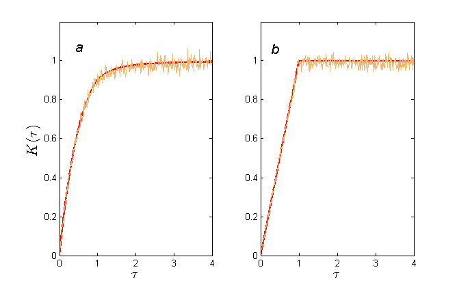
Figure 2: The form factor $K(\tau)$ (unfolded spectrum) for (a.) $3$-regular graphs numerical vs. the COE prediction. (b.) $3$-regular magnetic graphs vs. the CUE prediction.

The above comparisons between the predictions of RMT and the spectral statistics of the eigenvalues of $d$-regular graphs was based on the unfolding of the phases $\phi_{j}$ into the uniformly distributed phases $\theta_{j}$. As will become clear in the next sections, it is more natural to study here the fluctuations in the original spectrum and in particular the form factor

$$\widetilde{K}_{V}(t)=\frac{1}{V}\left\langle\left|\sum_{j=1}^{V}{\rm e}^{it\phi_{j}}\ \right|^{2}\ \right\rangle\ .$$ (25)

The transformation between the two spectra was effected by (14) which is one-to-one and its inverse is defined:

$$\phi=S(\theta)\doteq N_{KM}^{-1}\left(V\frac{\theta}{2\pi}\right)\ .$$ (26)

This relationship enables us to express $\widetilde{K}_{V}(t)$ in terms of $\ K_{V}(t)$. In particular, if $K_{V}(t)$ scales by introducing $\tau=\frac{t}{V}$ then,

$$\widetilde{K}(\tau=\frac{t}{V})=\frac{1}{\pi}\int_{0}^{\pi}d\theta K\left(\tau S^{{}^{\prime}}(\theta)\right).$$ (27)

The derivation of this identity is straightforward, and is described in A.

Figure (3) shows $\widetilde{K}(\tau=\frac{t}{V})=\widetilde{K}_{V}(t)$ computed by assuming that its unfolded analogue takes the RMT form (20) or (24), and it is compared with the numerical data for graphs with $d=10$. It is not a surprise that this way of comparing between the predictions of RMT and the data, shows the same agreement as the one observed previously.

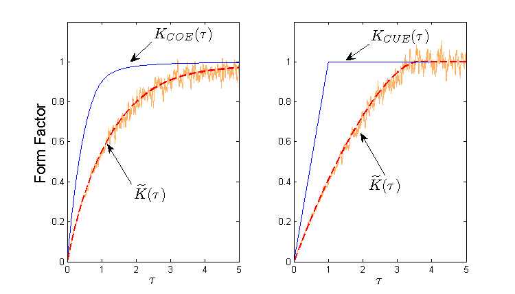
Figure 3: The form factor $\widetilde{K}(\tau)$ (original spectrum) for 10-regular graphs. The numerical results are presented vs. the expression (27) assuming RMT in the dashed line, and $K(\tau)$ (20, 24) in the solid line.

Remark: The rather unusual definition of the form factor for the original spectrum can be illustrated by the following example. Consider the Gaussian ensemble of $N$ dimensional symmetric matrices (GOE). Its spectrum (properly normalized) is supported on the interval $[-1,1]$ and the mean spectral density is given by Wigner’s semi-circle law. Mapping the spectrum onto the unit circle results in points which are non-uniformly distributed. One can generate the form factors $K(\tau)$ and $\widetilde{K}(\tau)$ from the original and unfolded spectra, and compare the numerical distributions to the predictions from COE. The corresponding $\widetilde{K}(\tau)$ is obtained from (27) in the limit $d\gg 1$.

With this summary of definitions and numerical data we prepared the background for the main results of the present work, where we use the trace formulae to express the spectral form factor in terms of the variance of the fluctuations in the counting of t-periodic nb walks on the two graph ensembles. In Chapter 2 we shall use the known properties of $t$-periodic nb walks to compute the leading term in the Taylor series of $\widetilde{K}(\tau)$, near $\tau=0$. In Chapter 3 we shall take the opposite direction, and by assuming that the spectral fluctuations for the graphs are given by RMT, we shall derive new expressions for the counting statistics of t-periodic nb walks on graphs. This approach is similar in spirit to the work of Keating and Snaith [12] who computed the mean moments of the Riemann $\zeta$ function on the critical line, assuming that the fluctuations of the Riemann zeros follow the predictions of RMT for the CUE ensemble.

2 From counting statistics of $t$-periodic orbits to RMT

In this section we shall establish a rigorous connection between the spectral properties of regular graphs and those predicted by RMT. To achieve this goal, we use the trace formula (8), where $y_{t}$ are defined by (9) or (10) for the two ensembles.

$$\tilde{\rho}(\mu)=\frac{1}{\pi}\sum_{t=3}^{\infty}\frac{y_{t}}{\sqrt{4(d-1)-\mu^{2}}}T_{t}\left(\frac{\mu}{2\sqrt{d-1}}\right)$$

Defining $\phi\equiv\arccos\left(\frac{\mu}{2\sqrt{d-1}}\right)$, and using the orthogonality of the cosine, we can extract $y_{t}$,

$$y_{t}=2\int_{0}^{\pi}\cos{(t\phi)}\tilde{\rho}(\phi)d\phi$$ (28)

And so:

$$\left\langle y^{2}_{t}\right\rangle=4\int_{0}^{\pi}\int_{0}^{\pi}\cos{(t\phi)}\cos{(t\psi)}\left\langle\tilde{\rho}(\phi)\tilde{\rho}(\psi)\right\rangle d\phi d\psi\ .$$ (29)

Recalling (56)

$$\widetilde{K}_{V}(s)\equiv 2V\int_{0}^{\pi}\int_{0}^{\pi}\cos(s\phi)\cos(s\psi)\langle\tilde{\rho}(\phi)\tilde{\rho}(\psi)\rangle d\phi d\psi\ ,$$ (30)

and comparing (29) and (30) we get:

$$\widetilde{K}_{V}(t)=\frac{V}{2}\left\langle y^{2}_{t}\right\rangle\ .$$ (31)

So far the treatment of the two ensembles was carried on the same formal footing. We shall now address each ensemble separately.

2.1 The form factor for the $\mathcal{G}_{V,d}$ ensemble

As was mentioned previously, it is useful to define the number of nb t-cycles on the graph as $C_{t}=\frac{Y^{(A)}_{t}}{2t}$ (in this definition, one does not distinguish between cycles which are conjugate to each other by time reversal). From combinatorial graph theory it is known that on average $\left\langle C_{t}\right\rangle=\frac{(d-1)^{t}}{2t}$ [6, 7, 8, 9]. Hence $\widetilde{K}$ can also be written as:

$$\widetilde{K}^{(A)}_{V}(t)=\frac{t}{V}\cdot\frac{\left\langle\left(C_{t}-\left\langle C_{t}\right\rangle\right)^{2}\right\rangle}{\left\langle C_{t}\right\rangle}\ .$$ (32)

The expression of the spectral form factor $\widetilde{K}^{(A)}_{V}(t)$ in terms of combinatorial quantities is the main result of the present work. In particular, it shows that the form factor is the ratio between the variance of $C_{t}$-the number of nb t-cycles - and its mean. This relation is valid for all $t$ in the limit $V\rightarrow\infty$.

For $t$ satisfying $t<log_{d-1}V$, it is known that asymptotically, for large $V$, the $C_{t}$’s are distributed as independent Poisson variables. For a Poisson variable, the variance and mean are equal. This implies that for $\tau=\frac{t}{V}\rightarrow 0$, $\widetilde{K}^{(A)}_{V}(t)=\tau$. Notice that the relation (27) implies $K_{V}(t)=2\widetilde{K}_{V}(t)$ for $\tau\rightarrow 0$ (see also 62).

Thus, for $\tau\ll 1$

$$K^{(A)}(\tau)=2\tau\ .$$ (33)

This result coincides with the COE prediction (20). It provides the first rigorous support of the connection, established so far numerically, between RMT and the spectral statistics of graphs . It is analogous to Berry’s “diagonal approximation” [13] in quantum chaos.

2.2 The form factor for the $\mathcal{G}^{M}_{V,d}$ ensemble

In the magnetic ensemble the matrices (2) are complex valued and Hermitian, which is tantamount to breaking time reversal symmetry. The relevant RMT ensemble in this case is the CUE.

In the ensuing derivation we shall take advantage of the statistical independence assumed for the magnetic phases which are uniformly distributed on the circle. Ensemble averaging will imply averaging over both the magnetic phases and the graphs.

Recall that $y^{(M)}_{t}$, in the case of magnetic graphs, was defined, by (10):

$$y^{(M)}_{t}=\frac{1}{V}\frac{Y_{t}^{(M)}}{(\sqrt{(d-1)})^{t}}\ \ ,\ \ Y^{(M)}_{t}=\sum_{\alpha}{\rm e}^{i\chi_{\alpha}}.$$

$Y^{(M)}_{t}$ is the sum of interfering phase factors contributed by the individual nb $t$-periodic walks on the graph. The phase factors of periodic walks which are related by time reversal are complex conjugated. Periodic walks which are self tracing (meaning that every bond on the cycle is traversed the same number of times in both directions), have no phase: $\chi_{\alpha}=0$. Using standard arguments from combinatorial graph theory one can show that for $t<\log_{d-1}V$, self tracing nb t-periodic walks are rare. Moreover, the number of $t$-periodic walks which are repetitions of shorter periodic walks can also be neglected. Hence

$$Y_{t}^{(M)}\approx 2t\textstyle\sum_{\alpha}^{{}^{\prime}}\cos(\chi_{\alpha})$$ (34)

where $\sum^{{}^{\prime}}$ includes summation over the nb $t$-cycles excluding self tracing and non-primitive cycles. The number of $t$-cycles on the graph is $C_{t}$, hence (34) has approximately $C_{t}$ terms. From (34) and the definition of $y_{t}^{(M)}$, it is easily seen that $\langle(y^{(M)}_{t})^{2}\rangle=\frac{1}{V^{2}(d-1)^{t}}4t^{2}\langle\left(\sum^{{}^{\prime}}\cos(\chi_{\alpha})\right)^{2}\rangle$. Averaging over the independent magnetic phases we get that

$$\widetilde{K}^{(M)}_{V}(t)=\frac{V}{2}\langle(y^{(M)}_{t})^{2}\rangle\approx\frac{t}{2V}\equiv\frac{\tau}{2}.$$ (35)

For $\tau\rightarrow 0$, and to leading order, $K=2\widetilde{K}$ (62). Hence

$$K^{(M)}(\tau)=\tau\ ,$$ (36)

which agrees with the CUE prediction.

3 Counting statistics of $t$-periodic cycles on $d$-regular graphs from RMT

In the previous section we made use of the known asymptotic statistics of $Y_{t}$ to show that the leading term in the expansion of $K_{V}(t)$ behaves as $g\tau$ where $g=1,2$ for the two graph ensembles. This property is consistent with the predictions of RMT. Had we known more about the counting statistics, we could make further predictions and compare them to RMT results. However, to the best of our knowledge we have exhausted what is known from combinatorial graph theory, and the only way to proceed would be to take the reverse approach, and assume that the form factor for graphs is given by the predictions of RMT, and see what this implies for the counting statistics. Checking these predictions from the combinatorial point of view is beyond our scope. However, we shall show that they are accurately supported by the numerical simulations.

The starting points for the discussion are the relations (31) and (27) which can be combined to give

$$\left\langle(y_{t})^{2}\right\rangle=\frac{2}{V}\widetilde{K}_{V}(t)=\frac{2}{V\pi}\int_{0}^{\pi}d\theta K\left(\tau S^{{}^{\prime}}(\theta)\right)\ .$$ (37)

Our strategy here will be to use for the unfolded form factor the known expressions from RMT (20) and (24) and compute $\left\langle(y_{t})^{2}\right\rangle$. This will provide an expression for the combinatorial quantities defined for each of the graph ensembles, and expanding in $\tau$ we shall compute the leading correction to their known asymptotic values.

To proceed, we have to analyze the integral (27) and expand it in powers of $\tau$ near $\tau=0$. For this purpose we have to recall the function $S(\theta)=N_{KM}^{-1}\left(V\frac{\theta}{2\pi}\right)$ (26). The inversion of the spectral counting function needs more attention near the end points of the support, where

$$N_{KM}(\phi)\underset{\phi\rightarrow 0}\longrightarrow\frac{2V}{3\pi}D\phi^{3};\ \ D\equiv\frac{d(d-1)}{(d-2)^{2}}\ .$$ (38)

Thus, in the vicinity of $\theta=0$

$$S(\theta)\approx S_{0}(\theta)=\left[\frac{3\theta}{4D}\right]^{\frac{1}{3}},$$ (39)

and $S^{\prime}$ which is singular near $0$ is

$$S^{{}^{\prime}}(\theta)\approx S_{0}^{{}^{\prime}}(\theta)=\frac{1}{4D}\ \left[\frac{4D}{3\theta}\right]^{\frac{2}{3}}.$$ (40)

Both RMT form factors take the value $1$ for argument values sufficiently larger than $1$. Hence the value of $\theta$ where the $\tau S^{\prime}(\theta)=1$ plays an important rôle. We shall denote it by $\theta_{m}(\tau)$, and for small values of $\tau$ it takes the value

$$\theta_{m}(\tau)=\frac{4D}{3}\cdot\left[\frac{\tau}{4D}\right]^{\frac{3}{2}}$$

.

This information suffices for the analytic derivations which will follow. However, for the numerical computation of $\widetilde{K}(\tau)$ for the entire range of $\tau$, we shall need a better approximation for $S(\theta)$ valid over the entire range of integration. This can be achieved by successive Newton-Raphson iterations. To second order,

$$S(\theta)=S_{0}+\frac{1}{8d(d-1)}\left(2\theta-2dS_{0}+2(d-2)\arctan\frac{d\tan\left(S_{0}\right)}{d-2}\right)\cdot\left(d^{2}+(d-2)^{2}\cot^{2}\left(S_{0}\right)\right).$$ (41)

The numerical error, induced by this approximation, is less than 5 percents, (it is less than 2 percents for $d>8$).

We now turn to the small $\tau$ domain. We shall treat the two ensembles separately starting with the magnetic ensemble since it is simpler.

3.1 Counting statistics for the $\mathcal{G}^{M}_{V,d}$ ensemble

The CUE form factor (24) is: $K_{CUE}(\tau)=\tau$ for $\tau<1$, and $K_{CUE}(\tau)=1$ for $1\leq\tau$. Therefore, we can divide the integral (27), in the following way:

$$\widetilde{K}^{(M)}(\tau)=\frac{1}{\pi}\left(\int_{0}^{\theta_{m}}d\theta+\int_{\theta_{m}}^{\pi}\tau S^{{}^{\prime}}(\theta)d\theta\right)=\frac{1}{\pi}\left(\theta_{m}+\frac{\pi\tau}{2}-\tau S(\theta_{m})\right)=$$ (42)

$$=\frac{\tau}{2}+\frac{1}{\pi}\left(\theta_{m}-\tau S(\theta_{m})\right)$$

Hence, the first two terms in the expansion of $\widetilde{K}(\tau)$ are

$$\widetilde{K}^{(M)}(\tau)=\frac{\tau}{2}+f_{1}(d)\tau^{\frac{3}{2}}+\ldots$$ (43)

where

$$f_{1}(d)=-\frac{1}{3\pi\sqrt{D}}\ .$$ (44)

Thus, the difference $(\widetilde{K}^{(M)}(\tau)-\frac{\tau}{2})/f_{1}(d)$, should scale for small $\tau$ as $\tau^{\frac{3}{2}}$ for all values of $d$. This data collapse is shown in figure (4).

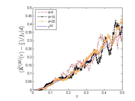
Figure 4: $(\widetilde{K}^{(M)}(\tau)-\frac{\tau}{2})/f_{1}(d)$ for various values of $d$ vs. the curve $\tau^{\frac{3}{2}}$.

3.2 Counting statistics for the $\mathcal{G}_{V,d}$ ensemble

Similar results can be obtained for the counting statistics of the $\mathcal{G}_{V,d}$ ensemble. Here, the relevant RMT form factor is the COE expression (20). The integral (27), is divided in the following way:

$$\widetilde{K}^{A}(\tau)=\frac{1}{\pi}\left(\int_{0}^{\theta_{m}}(2-\tau S^{{}^{\prime}}(\theta)\log{\frac{2\tau S^{{}^{\prime}}(\theta)+1}{2\tau S^{{}^{\prime}}(\theta)-1}})d\theta\right)$$ (45)

$$+\frac{1}{\pi}\left(\int_{\theta_{m}}^{\pi}2\tau S^{{}^{\prime}}(\theta)-\tau S^{{}^{\prime}}(\theta)\log{(2\tau S^{{}^{\prime}}(\theta)+1)}d\theta\right)$$ (46)

$$=\frac{1}{\pi}\left(2\theta_{m}+\pi\tau-2\tau S(\theta_{m})-\tau\int_{0}^{\theta_{m}}S^{{}^{\prime}}(\theta)\log{\frac{2\tau S^{{}^{\prime}}(\theta)+1}{2\tau S^{{}^{\prime}}(\theta)-1}}d\theta\right)$$ (47)

$$+\frac{1}{\pi}\left(-\tau\int_{\theta_{m}}^{\pi}S^{{}^{\prime}}(\theta)\log{(2\tau S^{{}^{\prime}}(\theta)+1)}d\theta\right),$$ (48)

We change variables to integrate over the new variable $x\equiv S(\theta)$. Denoting $S^{{}^{\prime}}(\theta)$ by $f(x)$, We get:

$$\widetilde{K}^{(A)}(\tau)=\frac{1}{\pi}\left(2\theta_{m}+\pi\tau-2\tau S(\theta_{m})-\tau\int_{0}^{S(\theta_{m})}dx\log{\frac{2\tau f(x)+1}{2\tau f(x)-1}}\right)$$ (49)

$$+\frac{1}{\pi}\left(-\tau\int_{S(\theta_{m})}^{\frac{\pi}{2}}dx\log{(2\tau f(x)+1)}\right),$$

At small values of $\tau$ (which imply small values of $\theta_{m}$), $f(x)=\frac{1}{4Dx^{2}}$. The first integral in (49) can be solved explicitly. In the second integral, we can restrict ourselves only to the interval in which $f(x)\propto\frac{1}{x^{2}}$ because the rest of the integral will only yield higher order terms in $\tau$. Therefore, we can also solve the second integral. Finally we get

$$\widetilde{K}^{(A)}(\tau)=\tau+f_{2}(d)\tau^{\frac{3}{2}}+\ldots$$ (50)

where

$$f_{2}(d)=\frac{1}{\sqrt{2D}}\left(\frac{2}{\pi}\cdot\text{arccoth}(\sqrt{2})-\frac{2\sqrt{2}}{3\pi}-1\right).$$ (51)

Thus, the difference $(\widetilde{K}^{(A)}(\tau)-\tau)/f_{2}(d)$, at small $\tau$, should scale as $\tau^{\frac{3}{2}}$ independently of $d$. This data collapse is shown in figure (5).

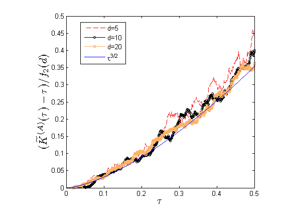
Figure 5: $(\widetilde{K}^{(A)}(\tau)-\tau)/f_{2}(d)$ for various values of $d$ vs. the curve $\tau^{\frac{3}{2}}$.

Using the above and (32) we can write,

$$\frac{\left\langle\left(C_{t}-\left\langle C_{t}\right\rangle\right)^{2}\right\rangle}{\left\langle C_{t}\right\rangle}=\frac{1}{\tau\pi}\int_{0}^{\pi}d\theta K_{COE}\left(\tau S^{{}^{\prime}}(\theta)\right)\underset{\tau\rightarrow 0}\longrightarrow 1+f_{2}(d)\sqrt{\tau}+\ldots$$ (52)

If the $C_{t}$’s were Poissonian random variables, the expansion above would terminate at $1$. Since it does not, we must conclude that the $C_{t}$’s are not Poissonian. The highest order deviation comes from the next order term in the expansion which is proportional to $\tau^{\frac{1}{2}}$. The coefficient, $f_{2}(d)$, is explicitly calculated above.

We can examine the behavior at another domain of $\tau$, namely $\tau>1$.
It can easily be shown that $S^{{}^{\prime}}(\theta)\geq\frac{d}{4(d-1)}$. Consequently, for $\tau>\frac{4(d-1)}{d}$, the argument of $K$ in (27) is larger than one, and so

$$\lim_{\tau\rightarrow\infty}\widetilde{K}^{(A)}(\tau)=1.$$ (53)

Combining this result with (32), provides the asymptotic of the variance-to-mean ratio:

$$\lim_{\tau\rightarrow\infty}\tau\frac{var(C_{t})}{\langle C_{t}\rangle}=1,\ \ \ for\ V,t\rightarrow\infty;\ \ \frac{t}{V}=\tau$$ (54)

This is a new interesting combinatorial result, since very little is known about the counting statistics of periodic orbits in the regime of $\tau>1$.

4 Discussion

The two main results of the present paper can be summarized as follows. First, we have shown that to leading order, the spectral statistics for graphs with time reversal symmetry is consistent with the COE, and when time reversal symmetry is broken, the CUE statistics come to play.
Second, by inverting the argument, and assuming RMT for the spectral statistics, we derived new results in graph theory, namely the deviation of the number of cycles from complete randomness, and the statistics at large $\tau$ . We do not know at this point how to interpret these results from a combinatorial point of view. This remains for now an open question. It is important to emphasize that unlike the standard approach in RMT, in this paper we have worked with the entire spectrum (bulk and edge states), not merely the bulk. As a result, effects of the edge states must be taken into account when trying to give a combinatorial answer to the questions posed above.
So far our rigorous results are rather limited. Yet, this work paves the way to further studies where the intricate relationship between combinatorial graph theory and RMT will be elucidated.

Appendix A The relation between $K(\tau)$ and $\widetilde{K}(\tau)$

The form factor (25) can be rewritten in the form

$$\widetilde{K}_{V}(s) \equiv \frac{2}{V}\left\langle\left|\sum_{j=1}^{V}\cos(s\phi_{j})\right|^{2}\right\rangle$$ (55)

$$= 2V\int_{0}^{\pi}\int_{0}^{\pi}\cos(s\phi)\cos(s\psi)\langle\rho(\phi)\rho(\psi)\rangle d\phi d\psi$$

The factor $V$ above is due to the normalization (1) of the spectral density. The smooth part of the spectral density does not encode any information about spectral fluctuations, so we are only interested in the fluctuating part, $\tilde{\rho}$. Thus,

$$\widetilde{K}_{V}(s)\equiv 2V\int_{0}^{\pi}\int_{0}^{\pi}\cos(s\phi)\cos(s\psi)\langle\tilde{\rho}(\phi)\tilde{\rho}(\psi)\rangle d\phi d\psi$$ (56)

We emphasize again that the main difference between $\widetilde{K}$ and the actual form factor, comes from the fact that the $\phi$’s are not uniformly distributed. Using the mapping $\phi=S(\theta)$ (26), we get:

$$\widetilde{K}_{V}(t)=2V\int_{0}^{2\pi}\int_{0}^{2\pi}\cos(tS(\theta))\cos(tS(\theta^{{}^{\prime}}))\langle\tilde{\rho}(\theta)\tilde{\rho}(\theta^{{}^{\prime}})\rangle d\theta d\theta^{{}^{\prime}}$$

The two-point correlation function is defined as $R_{2}(w)=\left(2\pi\right)^{2}\left\langle\tilde{\rho}(\theta)\tilde{\rho}(\theta+w\frac{2\pi}{V})\right\rangle$. In addition, we change variables to $\eta=\frac{\theta+\theta^{{}^{\prime}}}{2},w=\theta-\theta^{{}^{\prime}}$, and we expand the integrand up to first order in $w$, keeping in mind that $R_{2}(w)$ is only of significant magnitude if $w$ is small. We are thus left with:

$$\widetilde{K}_{V}(t)=\frac{V}{4\pi^{2}}\int_{0}^{2\pi}d\eta\int_{-2\pi}^{2\pi}dwR_{2}\left(\frac{wV}{2\pi}\right)\cdot\left[\cos(2tS(\eta))+\cos(twS^{{}^{\prime}}(\eta))\right]$$ (57)

The first integral is:

$$\frac{V}{4\pi^{2}}\int_{0}^{2\pi}d\eta\int_{-2\pi}^{2\pi}dwR_{2}\left(\frac{wV}{2\pi}\right)\cos(2tS(\eta))$$ (58)

$$=\frac{1}{2\pi}\int_{0}^{2\pi}d\eta\cos{(2tS(\eta))}\int_{-\infty}^{\infty}dsR_{2}(s)=\delta(\tau)$$ (59)

where we used $\int_{-\infty}^{\infty}dsR_{2}(s)=1$ (see for example ([11])).

The second integral is:

$$\frac{V}{4\pi^{2}}\int_{0}^{2\pi}d\eta\int_{-2\pi}^{2\pi}dwR_{2}\left(\frac{wV}{2\pi}\right)\cos(twS^{{}^{\prime}}(\eta))=\frac{1}{2\pi}\int_{0}^{2\pi}d\eta K\left(\tau S^{{}^{\prime}}(\eta)\right)$$ (60)

And we conclude that:

$$\widetilde{K}_{V}(t)=\delta(\tau)+\frac{1}{2\pi}\int_{0}^{2\pi}d\eta K\left(\tau S^{{}^{\prime}}(\eta)\right)$$ (61)

Where $\tau$ is defined as before, and $\widetilde{K}_{V}(t)$ admits the same scaling as in RMT: $\widetilde{K}(\tau=t/V)$. Finally, we drop the $\delta$-function term, and we take advantage of the fact that $S$ is symmetric around $\pi$ (this is a consequence of the Kesten-McKay measure being symmetric around zero). This completes the proof, and we end up with (27):

$$\widetilde{K}_{V}(\tau)=\frac{1}{\pi}\int_{0}^{\pi}d\theta K\left(\tau S^{{}^{\prime}}(\theta)\right)$$

Using this relation, we can prove that the slope of $K$ is twice that of $\widetilde{K}$ at $\tau=0$. Denote $\frac{{\rm d}K(\tau=0)}{{\rm d}\tau}=g$. Then,

$$\frac{{\rm d}\widetilde{K}(\tau=0)}{{\rm d}\tau}=\frac{g}{\pi}\int_{0}^{\pi}S^{{}^{\prime}}(\theta)d\theta=\frac{g}{2}$$ (62)

which proves the above.

References

References

- [1] I. Oren, A. Godel and U. Smilansky, Trace Formulae and Spectral Statistics for Discrete Laplacians on Regular Graphs (), J. Phys. A: Math. Theor. 42 415101 (2009).
- [2] D. Jacobson,S. Miller, I. Rivin and Z. Rudnick, Eigenvalue spacings for regular graphs, IMA Vol Math. Appl. 109 317 27 (1999).
- [3] Fritz Haake, Quantum Signatures Of Chaos. Springer-Verlag Berlin and Heidelberg, (2001).
- [4] H. Kesten Symmetric random walks on groups, Trans. Am. Math. Soc. 92, 336 354 (1959).
- [5] B.D. McKay, The expected eigenvalue distribution of a random labelled regular graph, Linear Algebr. Appl. 40, 203 216 (1981).
- [6] S. Janson, T. ŁUcZak and A. Ruciński, Random Graphs, John Wiley Sons, Inc. (2000).
- [7] N.C. Wormald, The asymptotic distribution of short cycles in random regular graphs, J. Combin. Theory, Ser. B 31 (1981) 168-182.
- [8] B. Bollobs, A probabilistic proof of an asymptotic formula for the number of labelled regular graphs, European J. Combin. 1 (1980) 311-316.
- [9] B.D. McKay, N.C. Wormald and B. Wysocka, Short cycles in random regular graphs, The electronic journal of combinatorics, volume 11. R66 (2004).
- [10] S. Sodin, The Tracy-Widom law for some sparse random matrices, Journal of Statistical Physics, Volume 136, Number 5 (2009), 834-841.
- [11] O. Bohigas, Random Matrix Theories and Chaotic Dynamics, in chaos and quantum physics, M.J. Giannoni, A. Voros and J. Zinn-Justin Editors, North-Holland Elsevier Science Publishers B.V, Amsterdam, The Netherlands, pp. 87-199.
- [12] J.P. Keating and N.C. Snaith, Random Matrix Theory and , Commun. Math. Phys. 214, 57 89 (2000).
- [13] M.V. Berry, Semiclassical Theory of Spectral Rigidity, Proc. Royal Soc. Lond A 400 (1985) 229.