On Vehicle Placement to Intercept Moving Targets

Abstract

We address optimal placement of vehicles with simple motion to intercept a mobile target that arrives stochastically on a line segment. The optimality of vehicle placement is measured through a cost function associated with intercepting the target. With a single vehicle, we assume that the target moves (i) with fixed speed and in a fixed direction perpendicular to the line segment, or (ii) to maximize the distance from the line segment, or (iii) to maximize intercept time. In each case, we show that the cost function is strictly convex, its gradient is smooth, and the optimal vehicle placement is obtained by a standard gradient-based optimization technique. With multiple vehicles, we assume that the target moves with fixed speed and in a fixed direction perpendicular to the line segment. We present a discrete time partitioning and gradient-based algorithm, and characterize conditions under which the algorithm asymptotically leads the vehicles to a set of critical configurations of the cost function.

1 Introduction

Vehicle placement to provide optimal coverage has received lot of recent attention. This paper addresses vehicle placement scenarios with the novelty of intercepting a mobile target generated randomly on a segment. Applications of this work are envisioned in border patrol wherein unmanned vehicles are placed to optimally intercept moving targets that cross a region under surveillance (cf. [Girard et al.(2004), Szechtman et al.(2008)]).

Vehicle placement problems are analogous to geometric location problems, wherein given a set of static points, the goal is to find supply locations that minimize a cost function of the distance from each point to its nearest supply location (cf. [Zemel(1984)]). For a single vehicle, the expected distance to a point that is randomly generated via a probability density function, is given by the continuous $1$–median function. The $1$–median function is minimized by a point termed as the median (cf. [Fekete et al.(2005)]). For multiple distinct vehicle locations, the expected distance between a randomly generated point and one of the locations is known as the continuous multi-median function (cf. [Drezner(1995)]). For more than one location, the multi-median function is non-convex, and thus determining locations that minimize the multi-median function is hard in the general case. [Cortés et al.(2004)] addressed a distributed version of a partition and gradient based procedure, known as the Lloyd algorithm, for deploying multiple robots in a region to optimize a multi-median cost function. [Schwager et al.(2009)] provided an adaptive control law to enable robots to approximate the density function from sensor measurements. [Martínez and Bullo(2006)] presented motion coordination algorithms to steer a mobile sensor network to an optimal placement. [Kwok and Martínez(2010)] presented a coverage algorithm for vehicles in a river environment. Related forms of the cost function have also appeared in disciplines such as vector quantization, signal processing and numerical integration (cf. [Gray and Neuhoff(1998), Du et al.(1999)]).

In mobile target scenarios, the cost for the vehicle is a function of relative locations, speeds and motion constraints considered. For an adversarial target, the optimal vehicle motion is obtained by solving a min-max pursuit-evasion game, in which the target seeks to maximize while the vehicle seeks to minimize a certain cost function. The vehicle strategy is a version of the classic proportional navigation guidance law (cf. [Guelman(1971)]). With constraints such as a wall in the playing space or non-zero capture distance, strategies with optimal intercept time have been derived in [Isaacs(1965)] and in [Pachter(1987)].

We consider a line segment on which a mobile target is generated via a known spatial probability density and one or multiple vehicles seek to intercept it. Knowledge about the density is a standard assumption in search problems (cf. [Stone(1975)]). The goal is to determine vehicle placements that minimize a cost function associated with the target motion. With a single vehicle, we consider a class of cost functions and establish its convexity, its smoothness and the existence of a unique global minimizer. We show that the cost functions associated with the target moving with fixed speed and in a fixed direction perpendicular to the line segment, and with the target seeking to maximize the distance from the segment, fall in the class of cost functions that we have analyzed. The cost function for target motion that maximizes the intercept time is shown to be proportional to the continuous $1$–median function. With multiple vehicles and the target moving with fixed speed perpendicular to the line segment, we first provide an algorithm to partition the line segment among the vehicles and characterize its properties. With the expected intercept time as the cost, we propose a Lloyd algorithm in which every vehicle computes its partition and descends the gradient of the cost computed over its partition. We characterize conditions under which the vehicles asymptotically reach a set of critical configurations.

In [Bopardikar et al.(2010)], we addressed optimal placement for a single vehicle with uniformly generated targets that have fixed speed and direction. This paper extends our work to include non-uniform generation density, adversarial target motion, and multiple vehicle scenario. Existing analyses of Lloyd algorithms (cf. [Cortés et al.(2004), Du et al.(1999)]) do not apply to this formulation due to a different form of the cost function.

This paper is organized as follows. The problem is formulated in Section 2. Single vehicle scenarios are addressed in Section 3. The multiple vehicle scenario is addressed in Section 4. The proofs of Lemmas 3.1, 4.5 and 4.8 are presented in the Appendix.

2 Problem Statement

We consider vehicles modeled with single integrator dynamics having unit speed. A target is generated at a random position $(x,0)$ on the segment $G:=[0,W]\times\{0\}$, termed the generator, via a specified probability density function $\phi:[0,W]\rightarrow{\mathbb{R}}_{\geq 0}$. We assume that the density $\phi$ is bounded, i.e., there exists an $M>0$ such that $\phi(x)\leq M,\forall x\in[0,W]$. The target moves with bounded speed $v<1$, and is intercepted or captured if a vehicle and the target are at the same point. We assume that the vehicles can sense the instantaneous position and velocity vector of the target. Target velocity information may be obtained using Doppler-based methods. The goal is to determine vehicle placements and corresponding capture motions that minimize a certain cost function based on the maneuvering abilities of the target. We consider the following cases.

2.1 Single Vehicle Case

We determine a location $\mathbf{p}\in{\mathbb{R}}\times{\mathbb{R}}_{\geq 0}$ that minimizes ${C}_{\textup{exp}}:{\mathbb{R}}\times{\mathbb{R}}_{\geq 0}\rightarrow{\mathbb{R}}$ given by

$${C}_{\textup{exp}}(\mathbf{p}):=\int_{0}^{W}C(\mathbf{p},x)\phi(x)dx,$$ (1)

where $C:{\mathbb{R}}\times{\mathbb{R}}_{\geq 0}\times[0,W]\rightarrow{\mathbb{R}}_{\geq 0}$ is an appropriately defined cost of the vehicle position $\mathbf{p}$. In what follows, we consider the following target motions.

(i) Constrained target: We assume that the target is constrained to move in the positive $Y$-direction with fixed speed $v<1$. From [Bopardikar et al.(2010)], the cost function $C$ is

$$T(\mathbf{p},x)=\frac{\sqrt{(1-v^{2})(X-x)^{2}+Y^{2}}}{1-v^{2}}-\frac{vY}{1-v^{2}},$$ (2)

where the quantity $1$ arises from normalizing the vehicle speed to unity, $\mathbf{p}:=(X,Y)$ and $T$ is the time taken for the vehicle to intercept the constrained target.

(ii) Adversarial target: We consider a differential pursuit evasion game in which the target (evader) seeks to maximize and the vehicle (pursuer) seeks to minimize any one of the following cost functions.

(a) Expected vertical height: The cost function $C$ is the vertical height $H(\mathbf{p},x)$, i.e., the distance of the target from the generator in the positive $Y$ direction, when the target is intercepted (cf. Figure 1).

(b) Expected intercept time: The cost function $C$ is the time interval $\mathbf{Ti}(\mathbf{p},x)$ before the target is intercepted (cf. Figure 1). In this formulation, we also assume that the target does not go below the X-axis.

The motions of the target and the vehicle are obtained from the solution of these differential games and will be addressed, along with formulae for $H$ and $\mathbf{Ti}$, in Section 3.2.

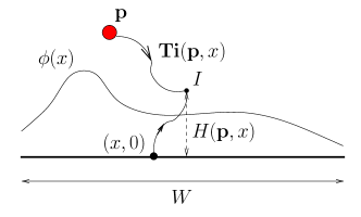
Figure 1: Adversarial target scenario. The vertical height $H$ is the distance of the intercept point $I$ from the generator. Due to unit speed of the vehicle, the intercept time $\mathbf{Ti}$ is equal to the distance covered by $\mathbf{p}$ until the target is intercepted.

2.2 Multiple Vehicles Case

We assume that the target translates in the positive $Y$-direction with speed $v<1$. As shown in Figure 2, given $m\geq 2$ vehicles having complete communication, the goal is to determine vehicle locations $\mathbf{p}_{i}\in[0,W]\times{\mathbb{R}}_{\geq 0}$, for every $i\in\{1,\dots,m\}$, that minimize the expected constrained travel time given by

$${T}_{\textup{exp}}(\mathbf{p}_{1},\dots,\mathbf{p}_{m}):=\int_{0}^{W}\min_{i\in\{1,\dots,m\}}T(\mathbf{p}_{i},x)\phi(x)dx,$$ (3)

where $T(\mathbf{p}_{i},x)$ is given by Eq. (2).

Figure 2: Intercepting a target moving with fixed speed $v$ perpendicular to the generator.

Remark 2.1 (Adversarial target scenarios)

The adversarial target counterparts of the multiple vehicle case are difficult to analyze theoretically. Section 4.4 provides some insight into the scenarios.

3 Single Vehicle Scenarios

In this section, we address optimal placement for a single vehicle in the scenarios mentioned in Section 2.1.

3.1 Cost functions for Expected Constrained Travel Time and Expected Vertical Height

We analyze cost functions given by Eq. (1), where the function $C$ has the form

$$C(X,Y,x):=a\sqrt{b(X-x)^{2}+Y^{2}}-cY,$$ (4)

and $a$, $b$, and $c$ are positive constants, with $a>c$. The constrained travel time $T$ (cf. Eq. (2)) has this form and we will show that the vertical height $H$ also has this form in Section 3.2.

Using $C$ as defined in Eq. (4), the partial derivatives of ${C}_{\textup{exp}}(X,Y)$ from Eq. (1) are given by

$$\frac{\partial{C}_{\textup{exp}}}{\partial X}=ab\int_{0}^{W}\frac{(X-x)\phi(x)}{\sqrt{b(X-x)^{2}+Y^{2}}}dx,$$ (5)

$$\frac{\partial{C}_{\textup{exp}}}{\partial Y}=aY\int_{0}^{W}\frac{\phi(x)}{\sqrt{b(X-x)^{2}+Y^{2}}}dx-c.$$ (6)

We first establish strict convexity of ${C}_{\textup{exp}}$.

Lemma 3.1 (Strict convexity of expected cost)

In the domain ${]0,W[}\times{\mathbb{R}}_{>0}$, the expected cost ${C}_{\textup{exp}}(X,Y)$

1. is continuous and convex in $X$ and $Y$, and

2. has a unique minimizer.

Statement (i) of Lemma 3.1 involves showing that the Hessian matrix of $C$ with respect to $X$ and $Y$ is positive semi-definite. The existence of a minimizer is established by showing that the partial derivatives of $C$ with respect to $X$ and $Y$ vanish inside ${]0,W[}\times{\mathbb{R}}_{>0}$. The uniqueness is established by assuming two distinct minimizers, using the convexity of $C$ and the necessary conditions for the two distinct locations to be minima to reach a contradiction.

Lemma 3.1 leads to the main result.

Theorem 3.2 (Minimizing expected cost)

From any initial vehicle location in ${\mathbb{R}}\times{\mathbb{R}}_{>0}$ and for any pobability density function $\phi$, assume that the vehicle motion obeys

$$\dot{\mathbf{p}}(t)=-\frac{\partial{C}_{\textup{exp}}}{\partial\mathbf{p}}(\mathbf{p}(t)).$$ (7)

The following statements hold:

1. the vehicle position $\mathbf{p}(t)$ remains in $[0,W]\times{\mathbb{R}}_{>0}$ at all times, and

2. the vehicle position $\mathbf{p}(t)$ converges to the unique global minimizer of ${C}_{\textup{exp}}$.

Theorem 3.2 answers the problem of minimizing the expected value of $T$, given by Eq. (2), with $a:=1/(1-v^{2})$, $b:=(1-v^{2})$ and $c:=v/(1-v^{2})$, and $a>c$. Except for special cases such as in Remark 3.3, it is difficult to provide analytical expressions for the minimizer $\mathbf{p}^{*}$ of ${T}_{\textup{exp}}(\mathbf{p}^{*})$.

Remark 3.3 (Equal target and vehicle speeds)

If the target and the vehicle have equal speeds, the optimal placement in $X$ which minimizes ${T}_{\textup{exp}}$ is at the centroid of the distribution $\phi$, with the optimal $Y$ given by

$$X^{*}={\int_{0}^{W}\phi(x)xdx};\,Y^{*}=\sqrt{{\int_{0}^{W}\phi(x)(X^{*}-x)^{2}dx}}.\quad\hbox{$\square$}$$

3.2 Optimal Placement for Adversarial Target

We now address the differential pursuit-evasion games stated in case (ii) of Section 2.1, and determine optimal vehicle placements.

3.2.1 Minimizing the Expected Vertical Height

Given an ordered pair of distinct points $\{\mathbf{q}_{1},\mathbf{q}_{2}\}$ in a plane and a scalar $\lambda\in{[0,1[}$, Apollonius circle (cf. [Isaacs(1965)]) is the set of points $\mathbf{w}$ in the plane that satisfy $\|\mathbf{q}_{2}-\mathbf{w}\|=\lambda\|\mathbf{q}_{1}-\mathbf{w}\|$. Letting the pursuer position $\mathbf{p}=:\mathbf{q}_{1}$, the target (evader) position be $\mathbf{q}_{2}$ and $v=:\lambda$, the following is an established result.

Proposition 3.4 (Apollonius circle during pursuit)

If the pursuer and the evader both travel straight toward a point $U$ on the Apollonius circle, then any new such circle, obtained from a pair of simultaneous intermediate positions of the pursuer and the evader, is tangent to the original circle at U, and is contained in the original circle.

For any evader strategy, the pursuit strategy that minimizes the vertical height (cf. [Isaacs(1965)]) is to choose the pursuer’s velocity vector such that the line joining the pursuer and the evader remains parallel at all times to the line joining their initial locations, while reducing the distance. So, for optimal vehicle placement, it suffices to determine the optimal evader strategy. Algorithm 1 summarizes the optimal evader strategy, shown in Figure 3.

Assumes: Pursuer at $(X,Y)$. Evader at $(x,0)$.

1

2Compute center and radius of the Apollonius circle:

$$O :=(O_{x},O_{y})=\Big{(}\frac{x-v^{2}X}{1-v^{2}},\frac{-v^{2}Y}{1-v^{2}}\Big{)},$$

$$R :=\frac{v}{1-v^{2}}\sqrt{(X-x)^{2}+Y^{2}}.$$

3Move towards the point $(O_{x},O_{y}+R)$ with speed $v$.

Algorithm 1 Move towards top-most

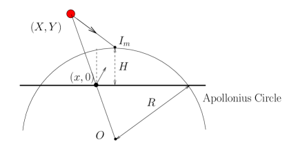
Figure 3: The evader strategy that maximizes $H$ is to move towards the top-most point on the Apollonius circle drawn initially.

The following result is immediate from Proposition 3.4.

Lemma 3.5 (Optimality of Move towards top-most)

The strategy move towards top-most is the evader’s optimal strategy and the optimal vertical height is

$$H(X,Y,x)=\frac{v}{1-v^{2}}\sqrt{(X-x)^{2}+Y^{2}}-\frac{v^{2}Y}{1-v^{2}}.$$

Comparing the expression for $H$ given by Lemma 3.5 with the definition of $C$ in Eq. (4), we have $a:=v/(1-v^{2})$, $b:=1$ and $c:=v^{2}/(1-v^{2})$, and $a>c$ since $v<1$. Thus, by applying Theorem 3.2, we obtain the following result.

Theorem 3.6 (Minimizing expected height)

From an initial location in ${\mathbb{R}}\times{\mathbb{R}}_{>0}$, assume that the vehicle motion obeys Eq. (7) with ${C}_{\textup{exp}}$ replaced by ${H}_{\textup{exp}}$, then the vehicle position $\mathbf{p}(t)$ converges to the unique global minimizer of ${H}_{\textup{exp}}$

3.2.2 Minimizing the Expected Intercept Time

The underlying differential game in this formulation is the classic wall pursuit game (cf. [Isaacs(1965)]). We present the main result for completeness.

Lemma 3.7 (Wall Pursuit game)

The evader strategy that maximizes the intercept time is to move towards the furthest point of the Apollonius circle on the $X$-axis.

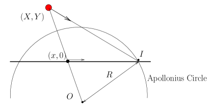
Figure 4: The evader strategy that maximizes $\mathbf{Ti}$ is to move towards the furthest point on the Apollonius circle drawn initially.

This optimal evader strategy is illustrated in Figure 4. Now, given a convex region $\mathcal{Q}\subset{\mathbb{R}}$ and a density function $\psi:\mathcal{Q}\rightarrow{\mathbb{R}}_{\geq 0}$, the median (cf. [Fekete et al.(2005)]) is the unique global minimizer $p^{*}$ of $\int_{\mathcal{Q}}|p-z|\psi(z)dz$.

We now present the main result of this section.

Theorem 3.8 (Optimality of the Median)

The median of the region $[0,W]\times\{0\}$ with the density function $\phi$ uniquely minimizes the expected intercept time.

Proof: From Lemma 3.7 and Pythagoras theorem,

$$\mathbf{Ti}(X,Y,x)=\frac{1}{v}\sqrt{R^{2}-\Big{(}\frac{vY}{1-v}\Big{)}^{2}}+\frac{1}{v}\left|\frac{x-vX}{1-v}-x\right|,$$

where $R$ is the radius of the Apollonius circle drawn at the initial instant. Since pursuer placement on the $X$-axis results into decreasing the intercept time $\mathbf{Ti}$, we have

$${\mathbf{Ti}}_{\textup{exp}}(X,0)=\frac{v+3}{1-v^{2}}\int_{0}^{W}|X-x|\phi(x)dx,$$

which is minimized uniquely by the median.   

4 The Case of Multiple Vehicles

We now address the multi-vehicle case from Section 2.2.

4.1 Dominance Region Partition

We introduce a generator partitioning procedure by defining dominance regions between each pair of vehicles. We will see that the resulting partition allows us to write the cost in Eq. (3) in a simplified form as in Eq. (9).

Definition 4.1 (Pairwise dominance region)

For $i,j\in\{1,\dots,m\}$, the pairwise dominance region $U_{ij}\subseteq[0,W]$ of $\mathbf{p}_{i}$ with respect to $\mathbf{p}_{j}$ is the set of initial target locations for which $\mathbf{p}_{i}$ takes lesser time to intercept the target than $\mathbf{p}_{j}$:

$$U_{ij}:=\{x\in[0,W]\,|\,T(\mathbf{p}_{i},x)\leq T(\mathbf{p}_{j},x)\}.$$

We now describe a procedure (summarized in Algorithm 2) to determine $U_{ij}$. Without loss of generality, assume that $X_{i}<X_{j}$. If $Y_{i}=Y_{j}$, i.e., the vehicles are at the same distance from the generator, then $U_{ij}$ is the piece of $G$ that lies in the half-plane that is formed by the perpendicular bisector of the segment joining $\mathbf{p}_{i}$ and $\mathbf{p}_{j}$ and which contains $\mathbf{p}_{i}$. Now if $Y_{i}<Y_{j}$, then we look for points $(x,0)$ in $G$ for which $T(\mathbf{p}_{i},x)\leq T(\mathbf{p}_{j},x)$. By setting $(1-v^{2})=:b$, Eq. (2) gives

$$\sqrt{b(X_{i}-x)^{2}+Y_{i}^{2}}-vY_{i}\leq\sqrt{b(X_{j}-x)^{2}+Y_{j}^{2}}-vY_{j}.$$ (8)

Eq. (8) simplifies to a quadratic in $x$ having real roots, which provides at most two points for the boundary between $U_{ij}$ and $U_{ji}$. To determine these boundary points, consider the perpendicular bisector of the segment joining $\mathbf{p}_{i}$ and $\mathbf{p}_{j}$, as shown in Figure 5.

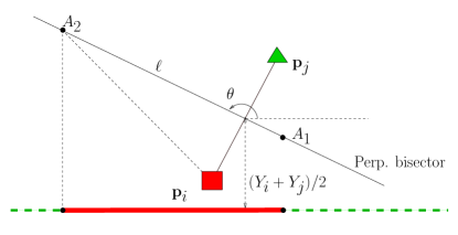
Figure 5: Pairwise dominance regions. The solid and dashed dominance regions belong to the square (red) and the triangle (green) vehicles respectively.

We look for points $A_{1}$ and $A_{2}$ on this bisector such that the distances of these points from the real line is $v$ times their respective distances from the vehicles. This leads to the following quadratic in $\ell$

$$4(\sin^{2}{\theta}-v^{2})\ell^{2}+4(Y_{i}+Y_{j})\sin{\theta}\ell=-(Y_{i}+Y_{j})^{2}+v^{2}\|\mathbf{p}_{i}-\mathbf{p}_{j}\|^{2},$$

where $\ell$ and $\theta:=\arctan_{2}((Y_{j}-Y_{i}),(X_{j}-X_{i}))+\pi/2$ are as shown in Figure 5. Let $\ell_{1}$ and $\ell_{2}$ be the roots of the above quadratic. Then the $Y$-coordinates of the candidate boundary points $A_{1}$ and $A_{2}$ are given by

$$[y_{1},\,y_{2}]^{T}=[1,\,1]^{T}(Y_{i}+Y_{j})/2+[\ell_{1},\,\ell_{2}]^{T}\sin{\theta}.$$

Now, $A_{1}$ and $A_{2}$ are both boundary points if and only if both have positive $Y$-coordinates. It can be shown that there exists at least one among them which has positive $Y$-coordinate. There arise two cases:

(i) If there are two candidate points $A_{1}$ and $A_{2}$ (as in Figure 5), then we look at their corresponding $X$ coordinates, $(x_{1},x_{2})$ given by Step 9. For $(x,0)\in G\cap[x_{1},x_{2}]\times\{0\}$, we have $T(\mathbf{p}_{i},x)\leq T(\mathbf{p}_{j},x)$, and thus $U_{ij}$ is $G\cap[x_{1},x_{2}]\times\{0\}$.

(ii) If there is only one candidate point $A_{1}$, then we look at its $X$ coordinate, $x_{1}$ given by Step 13. By assumption $X_{i}<X_{j}$, and hence for $(x,0)\in G\cap[-\infty,x_{1}]\times\{0\}$, we have $T(\mathbf{p}_{i},x)\leq T(\mathbf{p}_{j},x)$ and thus $U_{ij}$ is $G\cap[-\infty,x_{1}]\times\{0\}$.

Assumes: Distinct $\mathbf{p}_{i}=(X_{i},Y_{i})$, $\mathbf{p}_{j}=(X_{j},Y_{j})$.

1 if $Y_{i}=Y_{j}$, then

2       $U_{ij}:=\begin{cases}[0,(X_{i}+X_{j})/2],\,\,\,\text{ if }X_{i}<X_{j}\\ [(X_{i}+X_{j})/2,W],\text{ if }X_{i}>X_{j}\end{cases}$

3else

4       $\theta:=\arctan_{2}(Y_{j}-Y_{i},X_{j}-X_{i})+\pi/2$

5      [.3em] $\ell_{1,2}:=$ two roots of $0=4(\sin^{2}(\theta)-v^{2})\ell^{2}$

6        $+4(Y_{i}+Y_{j})\sin(\theta)\ell+(Y_{i}+Y_{j})^{2}-v^{2}\|\mathbf{p}_{i}-\mathbf{p}_{j}\|^{2}$

7      [.3em] $y_{1,2}:=(Y_{i}+Y_{j})/2+\sin(\theta)\ell_{1,2}$

8      [.3em]

9      if $y_{1}>0$ and $y_{2}>0$ then

10            $x_{1,2}:=(X_{i}+X_{j})/2+\cos(\theta)\ell_{1,2}$

11             $U_{ij}:=\begin{cases}[0,W]\cap[x_{1},x_{2}],\qquad\,\,\text{ if }Y_{i}<Y_{j}\\ [0,W]\setminus{]x_{1},x_{2}[},\qquad\,\,\,\text{ if }Y_{i}\geq Y_{j}.\end{cases}$

12      else

13            $k:=$ index in $\{1,2\}$ for which $y_{k}>0$

14             $x:=(X_{i}+X_{j})/2+\ell_{k}\cos(\theta)$

15            $U_{ij}:=\begin{cases}[0,W]\cap{]{-\infty},x]},\qquad\text{ if }X_{i}<X_{j}\\ [0,W]\cap{[x,+\infty[},\qquad\text{ if }X_{i}\geq X_{j}\end{cases}$

16      

Algorithm 2 Pairwise Dominance Region

Thus, we have established the following property.

Proposition 4.2 (Pairwise dominance region)

Given distinct locations $\mathbf{p}_{i}=(X_{i},Y_{i})$, $\mathbf{p}_{j}=(X_{j},Y_{j})$, if a target arrives at $(x,0)$, where $x\in U_{ij}$ generated by Algorithm 2, then $T(\mathbf{p}_{i},x)\leq T(\mathbf{p}_{j},x)$.

Similar to pairwise dominance regions, we introduce the concept of dominance region $\mathcal{V}_{i}\in\mathcal{P}([0,W])$ for the $i$th vehicle, for every $i\in\{1,\dots,m\}$, which is the set of $X$-coordinates of target locations for which $\mathbf{p}_{i}$ takes the minimum time to intercept of all vehicles.

Assuming complete communication between vehicles, Algorithm 2 is extended to determine the dominance region for a vehicle by (i) determining pairwise dominance regions between vehicles and, (ii) taking intersection of all pairwise dominance regions, as presented in Algorithm 3.

Assumes: Distinct locations $\{\mathbf{p}_{1},\dots,\mathbf{p}_{m}\}$.

1 foreach vehicle $j\in\{1,\dots,m\}\setminus\{i\}$, do

2       Determine $U_{ij}$ using Algorithm 2.

3      

4$\mathcal{V}_{i}=\bigcap_{j=1,\dots,m,j\neq i}U_{ij}$. ;

Algorithm 3 Dominance region

Algorithm 3 with three vehicles is illustrated in Figure 6. The next result follows due to disjoint interiors of dominance regions, and due to Proposition 4.2.

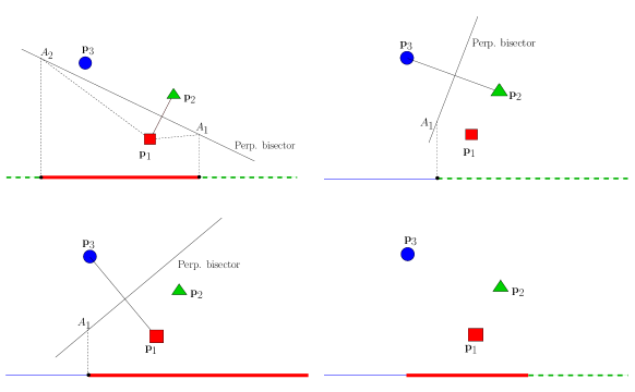
Figure 6: Algorithm 3 with three vehicles. The thick solid, the dashed and the thin solid dominance regions belong to the square (red), the triangle (green) and the round (blue) vehicles, respectively.

Proposition 4.3 (Optimality of dominance regions)

Given distinct vehicle positions and a target arrival,

(i) the dominance regions generated by Algorithm 3 form a partition of the generator.

(ii) The time taken to reach the target is minimized by the vehicle whose dominance region contains the target arrival location.

The dominance region of a vehicle may be empty if the vehicle is very far from the generating line as compared to the other vehicles (cf. first part of Figure 8). Conversely, all vehicles have non-empty dominance regions when they are all in $[0,W]\times{\mathbb{R}}_{\geq 0}$ and have the same $Y$-coordinates.

Since the dominance regions are set-valued functions of vehicle positions, we now provide some background on continuity of set-valued functions, and establish continuity of the dominance regions. This property will be used to analyze our gradient-based procedure. Let $\mathcal{E}:=[0,W]\times{\mathbb{R}}_{\geq 0}$, let $\mathcal{P}([0,W])$ be the set of all subsets of $[0,W]$, let $\mathcal{B}(r)$ be the closed ball of radius $r$ around the origin, and let $+$ denote the Minkowski sum of two sets. The domain of a set-valued map $F:X\rightrightarrows Z$ is the set of all $\mathbf{q}\in X$ such that $F(\mathbf{q})\neq\emptyset$. $F$ is upper (resp. lower) semi-continuous in its domain if, for every $\mathbf{q}$ in its domain and for every $\epsilon>0$, there exists a $\delta>0$ such that for every $\mathbf{z}\in\mathbf{q}+\mathcal{B}(\delta)$, $F(\mathbf{z})\subset F(\mathbf{q})+B(\epsilon)$ (resp. $F(\mathbf{q})\subset F(\mathbf{z})+B(\epsilon)$). $F$ is continuous if it is both upper and lower semi-continuous.

The pairwise dominance region between $\mathbf{p}_{i}$ and $\mathbf{p}_{j}$ is a set valued function $U_{ij}:\mathcal{E}^{2}\setminus\mathcal{S}_{ij}\rightrightarrows\mathcal{P}([0,W])$, where $\mathcal{S}_{ij}\subset\mathcal{E}^{2}$ is the set of coincident locations for $\mathbf{p}_{i}$ and $\mathbf{p}_{j}$. Similarly, the dominance region for vehicle $i$ is a set-valued map $\mathcal{V}_{i}:\mathcal{E}^{m}\setminus\mathcal{S}_{i}\rightrightarrows\mathcal{P}([0,W])$, where $\mathcal{S}_{i}\subset\mathcal{E}^{m}$ is the set of vehicle locations in which at least one other vehicle is coincident with $\mathbf{p}_{i}$. We now show that the dominance regions vary continuously with the vehicle positions.

Proposition 4.4 (Continuity of dominance regions)

(i) For every distinct $i$ and $j$ in the set $\{1,\dots,m\}$, the set valued map $U_{ij}$ is continuous in $\mathcal{E}^{2}\setminus\mathcal{S}_{ij}$.

(ii) For each vehicle $i\in\{1,\dots,m\}$, the set valued map $\mathcal{V}_{i}$ is continuous on its domain.

Proof: The roots of Eq. (8) which is a quadratic in $x$, vary continuously with $\mathbf{p}_{i}$ and $\mathbf{p}_{j}$. Thus, the map $U_{i,j}$ is continuous in $\mathcal{E}^{2}\setminus\mathcal{S}_{ij}$.

The domain of $\mathcal{V}_{i}$ is contained in the domain of $U_{ij}$ for every $j\neq i$. From part (i) of this Proposition, for every $j\neq i$, the set-valued map $U_{ij}$ is upper semi-continuous in $\mathcal{E}^{2}$. Thus, for every $j\neq i$, at every $\mathbf{q}$ in the domain of $\mathcal{V}_{i}$ and for every $\epsilon>0$, there exist $\delta_{ij}>0$ such that for every $\mathbf{z}\in\mathbf{q}+\mathcal{B}(\delta_{ij})$, $U_{ij}(\mathbf{z})\subset U_{ij}(\mathbf{q})+B(\epsilon)$. Given an $\epsilon>0$, by the choice of $\delta_{i}=\min\{\delta_{ij},\forall j\neq i\}$, we obtain that for every $\mathbf{z}\in\mathbf{q}+\mathcal{B}(\delta_{i})$, $\mathcal{V}_{i}(\mathbf{z})\subset\mathcal{V}_{i}(\mathbf{q})+B(\epsilon)$. Thus $\mathcal{V}_{i}$ is upper semi-continuous. Lower semi-continuity of $\mathcal{V}_{i}$ is established similarly and the result follows.   

4.2 Minimizing the Expected Constrained Travel Time

For distinct vehicle locations, Eq. (3) can be written as

$${T}_{\textup{exp}}(\mathbf{p}_{1},\dots,\mathbf{p}_{m})=\sum_{i=1}^{m}\int_{\mathcal{V}_{i}}T(\mathbf{p}_{i},x)\phi(x)dx,$$ (9)

where $\mathcal{V}_{i}$ is the dominance region of the $i$th vehicle. The gradient of ${T}_{\textup{exp}}$ is computed using the following formula, which allows each vehicle to compute the gradient of ${T}_{\textup{exp}}$ by integrating the gradient of $T$ over $\mathcal{V}_{i}$.

Lemma 4.5 (Gradient computation)

For all vehicle configurations such that no two vehicles are at coincident locations, the gradient of the expected time with respect to vehicle location $\mathbf{p}_{i}$ is

$$\frac{\partial{T}_{\textup{exp}}}{\partial\mathbf{p}_{i}}=\int_{\mathcal{V}_{i}}\frac{\partial T}{\partial\mathbf{p}_{i}}(\mathbf{p}_{i},x)\phi(x)dx.$$

Akin to similar results in [Bullo et al.(2009)], the proof involves writing the gradient of ${T}_{\textup{exp}}$ as a sum of two contributing terms. The first is the final expression, while the second is a number of terms which cancel out due to continuity of $T$ at the boundaries of dominance regions.

For $\mathbf{z}\in{\mathbb{R}}^{2}$, let $\operatorname{sat}:{\mathbb{R}}^{2}\rightarrow{\mathbb{R}}^{2}$ denote the saturation function, i.e., if $\|\mathbf{z}\|\leq 1$, then $\operatorname{sat}(\mathbf{z})=\mathbf{z}$; otherwise, $\operatorname{sat}(\mathbf{z})=\mathbf{z}/\|\mathbf{z}\|$. Inspired by the established Lloyd algorithm (cf. [Bullo et al.(2009)]), we present a discrete-time descent approach in Algorithm 4. The idea is to minimize ${T}_{\textup{exp}}$ by making each vehicle follow gradient descent over its dominance region. If the dominance region is empty, then the vehicle moves towards the generator, until it obtains a non-empty dominance region.

Assumes: Distinct locations $\{\mathbf{p}_{1},\dots,\mathbf{p}_{m}\}\in\mathcal{E}^{m}$

1

2foreach time $t\in{\mathbb{N}}$ do

3       Compute $\mathcal{V}_{i}(t)$ by Algorithm 3 as a function of $\{\mathbf{p}_{1}(t),\dots,\mathbf{p}_{m}(t)\}$

4       if $\mathcal{V}_{i}(t)$ is empty, then

5            Move in unit time to $(X_{i},Y_{i}-\min\{1,Y_{i}\})$;

6            

7      else

8             For $\tau\in[t,t+1]$, move according to $\displaystyle{\dot{\mathbf{p}}_{i}(\tau)=-\operatorname{sat}\Big{(}\int_{\mathcal{V}_{i}(t)}\frac{\partial}{\partial\mathbf{p}_{i}}T(\mathbf{p}_{i}(\tau),x)\phi(x)dx\Big{)}}$

9      

Algorithm 4 Lloyd descent for vehicle $i$

Next, we define critical configurations for the vehicles, which means that every vehicle is at the unique minimizer of the cost evaluated over its dominance region.

Definition 4.6 (Critical configuration)

A set of locations $\{\mathbf{p}_{1},\dots,\mathbf{p}_{m}\}$ is a critical configuration if,

$$\mathbf{p}_{i}=\operatornamewithlimits{argmin}_{\mathbf{z}\in\mathcal{E}}\int_{\mathcal{V}_{i}}T(\mathbf{z},x)\phi(x)dx,$$

for all $i\in\{1,\dots,m\}$, where $\{\mathcal{V}_{1},\dots,\mathcal{V}_{m}\}$ is the dominance region partition induced by $\{\mathbf{p}_{1},\dots,\mathbf{p}_{m}\}$.

We now state the main result of this section, that gives sufficient conditions under which the vehicles asymptotically reach a critical configuration using Algorithm 4.

Theorem 4.7 (Convergence of Lloyd descent)

Let $\gamma:{\mathbb{N}}\rightarrow{\mathbb{R}}^{2m}$ be the evolution of the $m$ vehicles according to Algorithm 4 and assume that no two vehicle locations become coincident in finite time or asymptotically. The following statements hold:

(i) the expected travel time $t\mapsto{T}_{\textup{exp}}(\gamma(t))$ is a non-increasing function of time;

(ii) if the dominance region $\mathcal{V}_{i}$ of any vehicle $i$ is empty at some time, then $\mathcal{V}_{i}$ will be non-empty within a finite time; and

(iii) if there exists a time $t$ such that every dominance region is non-empty for all times subsequent to $t$, then the vehicle locations converge to the set of critical dominance region configurations.

The assumptions of non-coincidence of vehicle locations and the non-emptiness of the dominance regions after a finite time ensure that the dominance regions are continuous functions of vehicle positions. The continuity of dominance regions in turn allows the LaSalle Invariance principle to be applicable. Further, it may be possible that the dominance region of a vehicle keeps alternating between being empty and non-empty under the action of Algorithm 4. However, it was observed through numerous simulations (e.g., see Figure 8) that after a finite time, the dominance region of every vehicle remained non-empty.

Proof: [Proof of Theorem 4.7] We begin by showing statement (i). In every iteration of Algorithm 4, step 2: does not increase the expected time ${T}_{\textup{exp}}$ due to the optimality of the dominance region partition, by Proposition 4.3. Step 4: does not change the ${T}_{\textup{exp}}$ as the associated dominance region is empty. Finally, step 6: does not increase ${T}_{\textup{exp}}$ as the vehicle is moving along the gradient descent flow of ${T}_{\textup{exp}}$. Thus, the expected time is non-increasing under Algorithm 4.

Statement (ii) follows from the fact that whenever $\mathcal{V}_{i}=\emptyset$ for vehicle $i$, due to step 4:, vehicle $i$ reaches the generator after finite time and therefore has a non-empty $\mathcal{V}_{i}$.

For non-empty $\mathcal{V}_{i}$, let $\mathcal{A}:\mathcal{X}\times\mathcal{P}([0,W])\rightarrow\mathcal{X}$, be the flow map of the differential equation at step 6: from time $t$ to time $t+1$. For statement (iii), consider the discrete-time dynamical system given by the tuple $(\mathcal{X},\mathcal{X}_{0},\mathcal{A})$, where $\mathcal{X}=\mathcal{E}^{m}$ and $\mathcal{X}_{0}\in\mathcal{E}^{m}$ is the set of initial vehicle positions.

We now apply the discrete-time LaSalle Invariance Principle (Theorem 1.19 in [Bullo et al.(2009)]), for which we verify the four assumptions as follows.

1. Existence of a positively invariant set: At every iteration of step 6:, each vehicle follows saturated gradient descent of a cost function belonging to the class of Eq. (4) over its dominance region fixed for the iteration. By the first statement of Theorem 3.2, each vehicle remains in $\mathcal{E}$ throughout the iteration, and therefore at all times. Thus, the set $\mathcal{E}^{m}$ is positively invariant for the system $(\mathcal{X},\mathcal{X}_{0},\mathcal{A})$.

2. Existence of a non-increasing function along $\mathcal{A}$: ${T}_{\textup{exp}}$ is non-increasing along $\mathcal{A}$, by statement (i) of this theorem.

3. Boundedness of all evolutions of $(\mathcal{X},\mathcal{X}_{0},\mathcal{A})$: Gradient descent keeps the $X$ coordinates bounded in $[0,W]$. It remains to show that the $Y$-coordinates of all vehicles remain bounded. Let us suppose the contrary. Then, there are two cases: (a) there exists a sequence of times on which at least one vehicle has its location bounded and at least one other vehicle, say vehicle $k$, has its $Y$-coordinate growing without limits; or (b) there exists a sequence of times on which the $Y$-coordinates of all vehicles grow unbounded. In case (a), after finite time, the dominance region $\mathcal{V}_{k}$ becomes empty, thus contradicting the assumption of statement (iii) of this theorem. If case (b) occurs, then there exists a subsequence of ${T}_{\textup{exp}}$ which grows unbounded, thus contradicting statement (i) of this theorem. Thus, all evolutions of $(\mathcal{X},\mathcal{X}_{0},\mathcal{A})$ are bounded.

4. Continuity of ${T}_{\textup{exp}}$ and $\mathcal{A}$: Continuity of ${T}_{\textup{exp}}$ follows from Eq.s (2) and (9). To verify continuity of $\mathcal{A}$, note that whenever $\mathcal{V}_{i}$ is non-empty, by Proposition 4.4, $\mathcal{V}_{i}$ is continuous with respect to vehicle locations. Thus, as long as $\mathcal{V}_{i}$ is non-empty, $\mathcal{A}$ is continuous as the integrand is continuous with respect to vehicle locations.

By LaSalle Invariance Principle, the evolutions of $(\mathcal{X},\mathcal{X}_{0},\mathcal{A})$ converge to a set of the form ${T}_{\textup{exp}}^{-1}(\kappa)\cap\mathcal{M}$, where $\kappa$ is a real constant and $\mathcal{M}$ is the largest positively invariant set in $\{x\in\mathcal{X}\,|\,{T}_{\textup{exp}}(\mathcal{A}(x))={T}_{\textup{exp}}(x)\}$. Since ${T}_{\textup{exp}}$ remains constant under action of $\mathcal{A}$ for the set of critical configurations, it is contained in a set of the form ${T}_{\textup{exp}}^{-1}(\kappa)\cap\mathcal{M}$. If a set of vehicle positions is not critical, then ${T}_{\textup{exp}}$ strictly decreases under the action $\mathcal{A}$, and therefore the set of vehicle positions is not contained in a set of ${T}_{\textup{exp}}^{-1}(\kappa)\cap\mathcal{M}$. Thus, the vehicles converge to the set of critical configurations.   

The next result gives a simple condition to identify an unstable critical configuration, which is an unstable equilibrium of Algorithm 4. Figure 7 illustrates this result.

Lemma 4.8 (Disconnected partitions are unstable)

A critical configuration is unstable if some vehicle has a disconnected dominance region.

The proof involves perturbing the position of a vehicle with a disconnected dominance region, and then showing that the gradient in the $X$ direction for that vehicle takes the vehicle away from the equilibrium configuration.

4.3 Simulations

We now present some simulations of Algorithm 4.

Examples of critical locations: We consider two vehicles, and a uniform target generation density, i.e., $\phi(x)=1/W$. From initial locations such as in the leftmost of Figure 7 wherein both vehicles having the same $X$-coordinate of $W/2$, but different $Y$-coordinates, the vehicles asymptotically approach the configuration in the center figure. However, a small perturbation to the vehicles leads to the configuration in the rightmost figure. Thus, this simulation illustrates Lemma 4.8. However, from most initial conditions, the vehicles converged to a critical configuration as in the rightmost figure.

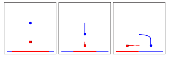
Figure 7: Algorithm 4 for uniform arrival density. The thick solid (red) and the thin solid (blue) dominance regions belong to the square and the round vehicles respectively. The vehicles first tend to an critical configuration (center figure). A perturbation to their positions makes them move to a stable critical configuration.

Non-uniform probability distribution: We consider three vehicles and the arrival probability density function,

$$\phi(x)=\begin{cases}{8x}/{W^{2}},&\text{ if }x\in{[0,W/4]},\\ {2}/{W}-{8}(x-{W}/{4})/(3W^{2}),&\text{ if }x\in{]W/4,W]}.\end{cases}$$

Initially, the round vehicle had an empty dominance region (Figure 8, left). After finite time, the round vehicle obtained a non-empty dominance region (Figure 8, center), after which all vehicles continued to have non-empty dominance regions. Thus, by Theorem 4.7, the vehicles converged to a critical configuration (Figure 8, right).

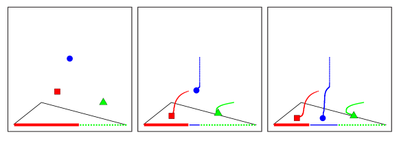
Figure 8: Algorithm 4 for non-uniform arrival density (black line). The dashed dominance region belongs to the triangle vehicle. Initially, the round vehicle has no dominance region.

4.4 Adversarial target motion: An insight

We now show that the partitioning procedure can be applied to the case of adversarial target. However, the dominance regions are difficult to characterize analytically. To see this, consider only two vehicles $\mathbf{p}_{1}$ and $\mathbf{p}_{2}$, and suppose the target is generated at $\mathbf{q}$. In order to maximize the vertical height (resp. intercept time), the optimal strategy for the target is (cf. [Isaacs(1965)]):

(i) Compute the Apollonius circles (ACs) with respect to the pursuer locations $\mathbf{p}_{1}$ and $\mathbf{p}_{2}$.

(ii) Move to the point with highest $Y$ coordinate (resp. furthest point) in the intersection of the ACs.

The strategy is illustrated in Figure 9. We partition the generator into: (i) $\mathcal{V}_{1}$ (resp. $\mathcal{V}_{2}$): Set of all locations $\mathbf{q}$ for which the AC of the target with respect to pursuer $\mathbf{p}_{1}$ (resp. $\mathbf{p}_{2}$) is entirely contained in the AC with respect to pursuer $\mathbf{p}_{2}$ (resp. $\mathbf{p}_{1}$); and (ii) $\mathcal{V}_{1,2}:=G\setminus(\mathcal{V}_{1}\cup\mathcal{V}_{2})$.

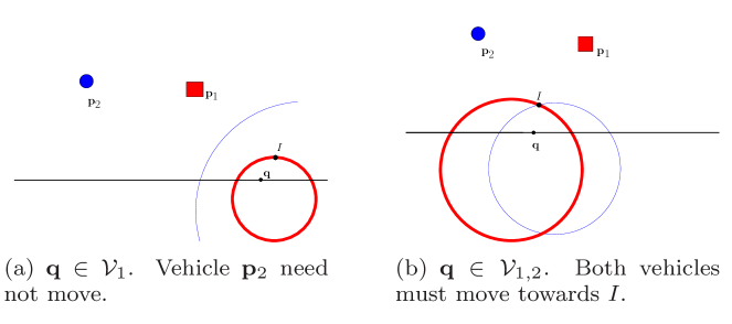
Figure 9: Generator partitioning to intercept an adversarial target.

The optimal pursuit strategy is to move $\mathbf{p}_{i}$ if $\mathbf{q}\in\mathcal{V}_{i}$, for some $i\in\{1,2\}$, and to move both $\mathbf{p}_{1}$ and $\mathbf{p}_{2}$ if $\mathbf{q}\in\mathcal{V}_{1,2}$. The average cost ${C}_{\textup{exp}}(\mathbf{p}_{1},\mathbf{p}_{2})$ can be written as

$${C}_{\textup{exp}}=\sum_{i=1}^{2}\int_{\mathcal{V}_{i}}C(\mathbf{p}_{i},x)\phi(x)dx+\int_{\mathcal{V}_{1,2}}C(\mathbf{p}_{1},\mathbf{p}_{2},x)\phi(x)dx.$$

The gradient of the first term is similar to that in Lemma 4.5. But, the second term $C(\mathbf{p}_{1},\mathbf{p}_{2},x)$ is difficult to characterize in the form of an analytical expression. Thus, the adversarial case is a challenging future direction.

5 Conclusions and Future Directions

We addressed the problem of optimally placing vehicles having simple motion in order to intercept a mobile target that arrives stochastically on a line segment. For a single vehicle, we determined unique optimal placements when target motion was either constrained, i.e., with fixed speed and direction, or adversarial. For the multiple vehicle scenario and with constrained motion targets, we characterized conditions under which a partition and gradient based algorithm takes the vehicles asymptotically to the set of critical points of the cost function.

A future direction is to consider numerical methods for the multiple vehicles with adversarial targets. Another direction is to consider stochastic target motion.

Appendix

In this Appendix, we provide complete proofs of Lemmas 3.1, 4.5 and 4.8.

Proof of Lemma 3.1: The first claim follows by verifying that the Hessian matrix of $C$ with respect to $X$ and $Y$ is positive semi-definite in the domain ${]0,W[}\times{\mathbb{R}}_{>0}$.

For the second claim, we need to show existence and uniqueness of a minimizer in the domain ${]0,W[}\times{\mathbb{R}}_{>0}$.

1. Existence: We show that a minimizer cannot lie on the boundary or outside of the domain $[0,W]\times{\mathbb{R}}_{\geq 0}$. We begin by showing that $Y^{*}$ exists and is finite. Taking the limit of ${C}_{\textup{exp}}(X,Y)$ as $Y\to+\infty$,

$$\liminf_{Y\to+\infty}{C}_{\textup{exp}}(X,Y)\geq\liminf_{Y\to+\infty}(a-c)Y\int_{0}^{W}\phi(x)dx=+\infty,$$

since by assumption, $a>c$. Thus, $Y^{*}$ exists and is finite.

Finally, to show that a minimizer lies in ${]0,W[}\times{\mathbb{R}}_{>0}$, we need to prove two statements: (a) $Y^{*}\neq 0$, and (b) $X^{*}\in{]0,W[}$. To show (a), Eq. (6) along with the assumption $\phi(x)\leq M$, for every $x\in[0,W]$, yields

$$\frac{\partial{C}_{\textup{exp}}}{\partial Y} \leq MYa\int_{0}^{W}\frac{dx}{\sqrt{b(X-x)^{2}+Y^{2}}}-c$$

$$\leq\frac{MYa}{\sqrt{b}}(\log(W+\sqrt{W^{2}+Y^{2}/b})-\log(Y/\sqrt{b}))-c.$$

Thus, $\limsup_{Y\to 0^{+}}{\partial{C}_{\textup{exp}}}/{\partial Y}\leq-c$. Thus, for $Y$ near zero, the gradient of ${C}_{\textup{exp}}$ points in the negative $Y$-direction, implying that $Y^{*}\neq 0$.

To show (b), we first observe that for a given $Y$, in the limit as $X\to\pm\infty$, ${C}_{\textup{exp}}\to+\infty$, and therefore $X^{*}$ must be bounded. Finally, the claim follows since the partial derivative of ${C}_{\textup{exp}}$ with respect to $X$ is strictly negative for $X\leq 0$ and is strictly positive for $X\geq W$.

Facts (a) and (b) coupled with convexity of ${C}_{\textup{exp}}$ with respect to $X$ and $Y$ establish the existence part.

2. Uniqueness: Let there be two locations $(X_{1},Y_{1})$ and $(X_{2},Y_{2})$ that minimize the expected cost. Since the expected cost ${C}_{\textup{exp}}$ is convex in $X$ and $Y$, a convex combination of $(X_{1},Y_{1})$ and $(X_{2},Y_{2})$ also minimizes ${C}_{\textup{exp}}$. Thus, the necessary conditions for minimum are satisfied by
$(\bar{X}(\alpha),\bar{Y}(\alpha)):=(\alpha X_{1}+(1-\alpha)X_{2},\alpha Y_{1}+(1-\alpha)Y_{2})$, for every $\alpha\in[0,1]$. Thus,

$$\int_{0}^{W}\frac{(\bar{X}(\alpha)-x)\phi(x)}{\sqrt{(b\bar{X}(\alpha)-x)^{2}+\bar{Y}(\alpha)^{2}}}dx =0,$$

$$\int_{0}^{W}\frac{\bar{Y}(\alpha)\phi(x)}{\sqrt{b(\bar{X}(\alpha)-x)^{2}+\bar{Y}(\alpha)^{2}}}dx =\frac{c}{a}.$$

Since the above conditions hold for every $\alpha\in[0,1]$, the partial derivatives of the above conditions evaluated at $\alpha=0$, must equal zero, which yields

$$\int_{0}^{W}\frac{(X_{2}-x)Y_{2}(Y_{1}-Y_{2})-Y_{2}^{2}(X_{1}-X_{2})}{(b(X_{2}-x)^{2}+Y_{2}^{2})^{3/2}}\phi(x)dx=0,$$

$$\int_{0}^{W}\frac{(X_{2}-x)Y_{2}(X_{1}-X_{2})-(Y_{1}-Y_{2})(X_{2}-x)^{2}}{(b(X_{2}-x)^{2}+Y_{2}^{2})^{3/2}}\phi(x)dx$$

$$=0,$$

where $\phi(x)/(b(X_{2}-x)^{2}+Y_{2}^{2})^{3/2}=:f(X_{2},Y_{2},x)$ is strictly positive for $Y_{2}>0$. Multiplying the first equation by $(X_{1}-X_{2})$, the second by $(Y_{1}-Y_{2})$, and adding the equations,

$$\int_{0}^{W}f(X_{2},Y_{2},x)(Y_{2}(X_{1}-X_{2})-(X_{2}-x)(Y_{1}-Y_{2}))^{2}dx=0.$$

Since $f(X_{2},Y_{2},x)\geq 0$, we must have $Y_{2}(X_{1}-X_{2})-(X_{2}-x)(Y_{1}-Y_{2})=0$, for every $x$ at which $f(X_{2},Y_{2},x)>0$, which is feasible only if $X_{1}-X_{2}=0$ and $Y_{1}-Y_{2}=0$.

Parts 1 and 2 complete the proof for the second claim.   

Proof of Lemma 4.5: Let $\mathbf{p}_{j}$ be termed as a neighbor of $\mathbf{p}_{i}$, i.e., $j\in$ neigh$(i)$, if $\mathcal{V}_{i}\cap\mathcal{V}_{j}$ is non-empty. Then,

$$\frac{\partial{T}_{\textup{exp}}}{\partial\mathbf{p}_{i}}=\frac{\partial}{\partial\mathbf{p}_{i}}\int_{\mathcal{V}_{i}}T(\mathbf{p}_{i},x)\phi(x)dx+\sum_{j\text{ neigh }(i)}\frac{\partial}{\partial\mathbf{p}_{i}}\int_{\mathcal{V}_{j}}T(\mathbf{p}_{j},x)\phi(x)dx,$$

Now, let $\mathcal{V}_{i}=\bigcup_{l=1,\dots,n_{i}}[a_{l},b_{l}]$, for some finite integer $n_{i}$. Then, there are two cases:

1. Every boundary point in the interior of $[0,W]$ belong to the dominance region of exactly two vehicles: In this case, all boundary points $a_{l}$ and $b_{l}$ are differentiable with respect to $\mathbf{p}_{i}$. Therefore, by Leibnitz’s Rule,

$$\frac{\partial}{\partial\mathbf{p}_{i}}\int_{\mathcal{V}_{i}}T(\mathbf{p}_{i},x)\phi(x)dx=\int_{\mathcal{V}_{i}}\frac{\partial T}{\partial\mathbf{p}_{i}}(\mathbf{p}_{i},x)\phi(x)dx+\sum_{l=1}^{n_{i}}T(\mathbf{p}_{i},b_{l})\frac{\partial b_{l}}{\partial\mathbf{p}_{i}}-T(\mathbf{p}_{i},a_{l})\frac{\partial a_{l}}{\partial\mathbf{p}_{i}}.$$

Unless $a_{1}=0$, or $b_{n_{i}}=W$ (in which case the partial derivatives with respect to $\mathbf{p}_{i}$ are zero), for every $l\in\{1,\dots,n_{i}\}$, there exist some $j\in$ neigh$(i)$ and some $k\in$ neigh$(i)$, such that

$$\frac{\partial}{\partial\mathbf{p}_{i}}\int_{\mathcal{V}_{j}}T(\mathbf{p}_{j},x)\phi(x)dx =-T(\mathbf{p}_{j},b_{l})\frac{\partial b_{l}}{\partial\mathbf{p}_{i}},$$ (10)

$$\text{and, }\frac{\partial}{\partial\mathbf{p}_{i}}\int_{\mathcal{V}_{k}}T(\mathbf{p}_{k},x)\phi(x)dx =T(\mathbf{p}_{k},a_{l})\frac{\partial a_{l}}{\partial\mathbf{p}_{i}},$$

where we have made use of Leibnitz’s Rule. Due to the continuity of $T$ at the boundary points, we obtain

$$T(\mathbf{p}_{j},b_{l})=T(\mathbf{p}_{i},b_{l}),\quad T(\mathbf{p}_{k},a_{l})=T(\mathbf{p}_{i},a_{l}),$$

and on summation,

$$\sum_{j\in\text{ neigh }(i)}\frac{\partial}{\partial\mathbf{p}_{i}}\int_{\mathcal{V}_{j}}T(\mathbf{p}_{j},x)\phi(x)dx+\sum_{l=1}^{n_{i}}T(\mathbf{p}_{i},b_{l})\frac{\partial b_{l}}{\partial\mathbf{p}_{i}}-T(\mathbf{p}_{i},a_{l})\frac{\partial a_{l}}{\partial\mathbf{p}_{i}}=0.$$

The proof is complete for this case.

2. Some $b_{l}$ (or $a_{l}$) belongs to the dominance regions of $\mathbf{p}_{i}$ and at least two other vehicles: Let $\mathbf{p}_{j}$ and $\mathbf{p}_{r}$ be two of these vehicles. We perturb the position of $\mathbf{p}_{i}$ in a direction $v$ by a small distance $\epsilon$. We claim that the boundary term $T(\mathbf{p}_{i},b_{l})\partial b_{l}/\partial\mathbf{p}_{i}$ is cancelled independent of the choice of the direction $v$. The following two possibilities arise (cf. Figure 10): either the point $b_{l}$ moves to the right or $b_{l}$ moves to the left by some distance $\delta(\epsilon)$. The steps for the former possibility are exactly identical to Case 1. In the latter possibility, we can write Eq. (10), if the interval $[b_{l}-\delta,b_{l}]$ belongs to $\mathcal{V}_{j}(\mathbf{p}_{1},\dots,\mathbf{p}_{i}+\epsilon v,\dots,\mathbf{p}_{m})$, or we can write Eq. (10) with $j$ replaced by $r$, if the interval $[b_{l}-\delta,b_{l}]$ belongs to $\mathcal{V}_{r}(\mathbf{p}_{1},\dots,\mathbf{p}_{i}+\epsilon v,\dots,\mathbf{p}_{m})$. Thus, in both of these possibilities, the steps from case 1 apply leading to the cancellation of all the boundary terms.

This completes the proof.   

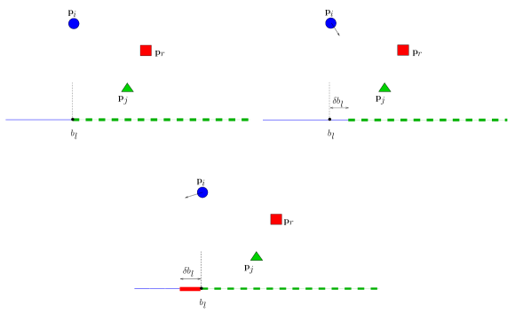
Figure 10: Illustration of case 2 in the proof of Lemma 4.5. In the first figure, the point $b_{l}$ belongs to the dominance regions of $\mathbf{p}_{i}$, $\mathbf{p}_{j}$ and $\mathbf{p}_{r}$. The second and third figures show how the dominance regions would change when $\mathbf{p}_{i}$ is perturbed in different directions. The thick solid, the dashed and the thin solid dominance regions belong to the square (red), the triangle (green) and the round (blue) vehicles, respectively.

Proof of Lemma 4.8: We first prove the result for the case of two vehicles. Let $\{\mathbf{p}_{1}^{*},\mathbf{p}_{2}^{*}\}$ be a critical dominance region configuration in which $\mathbf{p}_{1}$ has its dominance region disconnected. Let the dominance regions be

$$\mathcal{V}_{1}=[A,B],\quad\mathcal{V}_{2}=[0,A]\cup[B,W].$$

Perturb $\mathbf{p}_{1}$ by a small distance $\delta X$in the positive $X$ direction, as shown in Figure 11.

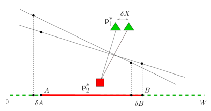
Figure 11: Illustrating instability of critical dominance region configuration having a disconnected dominance region.

From continuity of the dominance regions, we have

$$\mathcal{V}_{1}=[A-\delta A,B-\delta B],\,\mathcal{V}_{2}=[0,A-\delta A]\cup[B-\delta B,W],$$

where $\delta A$ and $\delta B$ are positive and sufficiently small. Let $I_{2}(x,X_{2},Y_{2}):=(X_{2}-x)\phi(x)/\sqrt{(1-v^{2})(X_{2}-x)^{2}+Y_{2}^{2}}$. Evaluating the partial derivatives in $X$ for $\mathbf{p}_{2}$,

$$(1-v^{2})\frac{\partial}{\partial X}T_{2}=\int_{A-\delta A}^{B-\delta B}I_{2}dx,$$

Upon further simplification,

$$(1-v^{2})\frac{\partial T_{2}}{\partial X} =\int_{A-\delta A}^{A}I_{2}dx+\int_{A}^{B}I_{2}dx-\int_{B-\delta B}^{b}I_{2}dx$$

$$=\int_{A-\delta A}^{A}I_{2}dx-\int_{B-\delta B}^{B}I_{2}dx,$$ (11)

as the sum of the first two terms is zero from the necessary condition for $\mathbf{p}_{2}^{*}$ to be a minimum. For sufficiently small $\delta X$, there exist $\delta A$ and $\delta B$ such that $I_{2}>0$ on the interval $[0,A-\delta A]$ and $I_{2}<0$ on the interval $[B-\delta B,B]$, since $X_{2}-x>0$ and $X_{2}-x<0$ respectively on the two intervals. Thus, $\partial T_{2}/\partial X>0$ when $\mathbf{p}_{1}$ is displaced to $(X_{1}+\delta X,Y_{1})$, which implies the direction of gradient descent in $X$ is the negative $X$ direction for $\mathbf{p}_{2}$, and similarly is the positive $X$ direction for $\mathbf{p}_{1}$. Thus, the critical configuration is unstable.

In the case of $m>2$ vehicles, let the dominance regions of $\mathbf{p}_{1}$ and $\mathbf{p}_{2}$ share at least one point. Since both terms on the right hand side of Eq. (Appendix) are positive, the direction of gradient descent in $X$ is the negative direction for $\mathbf{p}_{2}$ independent of the fact whether the dominance regions of $\mathbf{p}_{1}$ and $\mathbf{p}_{2}$ share one or two common points.

References

- [Bopardikar et al.(2010)] Bopardikar, S. D., Smith, S. L., Bullo, F., Hespanha, J. P., 2010. Dynamic vehicle routing for translating demands: Stability analysis and receding-horizon policies. IEEE Transactions on Automatic Control 55 (11), 2554–2569.
- [Bullo et al.(2009)] Bullo, F., Cortés, J., Martínez, S., 2009. Distributed Control of Robotic Networks. Applied Mathematics Series. Princeton University Press, available at http://www.coordinationbook.info.
- [Cortés et al.(2004)] Cortés, J., Martínez, S., Karatas, T., Bullo, F., 2004. Coverage control for mobile sensing networks. IEEE Transactions on Robotics and Automation 20 (2), 243–255.
- [Drezner(1995)] Drezner, Z. (Ed.), 1995. Facility Location: A Survey of Applications and Methods. Series in Operations Research. Springer.
- [Du et al.(1999)] Du, Q., Faber, V., Gunzburger, M., 1999. Centroidal Voronoi tessellations: Applications and algorithms. SIAM Review 41 (4), 637–676.
- [Fekete et al.(2005)] Fekete, S. P., Mitchell, J. S. B., Beurer, K., 2005. On the continuous Fermat–Weber problem. Operations Research 53 (1), 61 – 76.
- [Girard et al.(2004)] Girard, A. R., Howell, A. S., Hedrick, J. K., Dec. 2004. Border patrol and surveillance missions using multiple unmanned air vehicles. In: IEEE Conf. on Decision and Control. Paradise Island, Bahamas, pp. 620–625.
- [Gray and Neuhoff(1998)] Gray, R. M., Neuhoff, D. L., 1998. Quantization. IEEE Transactions on Information Theory 44 (6), 2325–2383, Commemorative Issue 1948-1998.
- [Guelman(1971)] Guelman, M., 1971. A qualitative study of proportional navigation. IEEE Transactions on Aerospace and Electronic Systems 7 (4), 637–643.
- [Isaacs(1965)] Isaacs, R., 1965. Differential Games. Wiley.
- [Kwok and Martínez(2010)] Kwok, A., Martínez, S., 2010. A coverage algorithm for drifters in a river environment. In: American Control Conference. Baltimore, MD, pp. 6436–6441.
- [Martínez and Bullo(2006)] Martínez, S., Bullo, F., 2006. Optimal sensor placement and motion coordination for target tracking. Automatica 42 (4), 661–668.
- [Pachter(1987)] Pachter, M., 1987. Simple motion pursuit-evasion in the half-plane. Computers and Mathematics with Applications 13 (1-3), 69–82.
- [Schwager et al.(2009)] Schwager, M., Rus, D., Slotine, J. J., 2009. Decentralized, adaptive coverage control for networked robots. International Journal of Robotics Research 28 (3), 357–375.
- [Stone(1975)] Stone, L. D., 1975. Theory of Optimal Search. Operations Research Society of America.
- [Szechtman et al.(2008)] Szechtman, R., Kress, M., Lin, K., Cfir, D., 2008. Models of sensor operations for border surveillance. Naval Research Logistics 55 (1), 27–41.
- [Zemel(1984)] Zemel, E., 1984. Probabilistic analysis of geometric location problems. SIAM Journal on Algebraic and Discrete Methods 6 (2), 189–200.