Network Conduciveness with Application to the Graph-Coloring and Independent-Set Optimization Transitions

Abstract

We introduce the notion of a network’s conduciveness, a probabilistically interpretable measure of how the network’s structure allows it to be conducive to roaming agents, in certain conditions, from one portion of the network to another. We exemplify its use through an application to the two problems in combinatorial optimization that, given an undirected graph, ask that its so-called chromatic and independence numbers be found. Though NP-hard, when solved on sequences of expanding random graphs there appear marked transitions at which optimal solutions can be obtained substantially more easily than right before them. We demonstrate that these phenomena can be understood by resorting to the network that represents the solution space of the problems for each graph and examining its conduciveness between the non-optimal solutions and the optimal ones. At the said transitions, this network becomes strikingly more conducive in the direction of the optimal solutions than it was just before them, while at the same time becoming less conducive in the opposite direction. We believe that, besides becoming useful also in other areas in which network theory has a role to play, network conduciveness may become instrumental in helping clarify further issues related to NP-hardness that remain poorly understood.

PACS numbers: 89.20.-a, 89.70.-a, 89.75.-k.

1 Introduction

The past decade has seen an impressive growth in the science of complex networks, understood as the branch of scientific inquiry which, by merging well established notions and techniques from the theory of graphs and from statistical physics, addresses the interplay of structure and function in the large, essentially unstructured networks that occur in a wide variety of domains. The latter have encompassed several instances in many biological, social, and technological fields, and have yielded an equally variegated array of results that the reader can now refer to in books and paper collections such as [8, 21, 6].

One common methodological thread in all these studies has been the definition of a graph to represent the interactions among certain entities in the domain of interest, followed by the analysis of mathematical descriptors of some of the graph’s properties as averages over a number of graphs generated according to some random-graph model thought to represent the phenomenon under consideration. Thus have emerged important finds regarding some networks’ characterization as small-world structures, or as scale-free structures, as well as powerful structural indicators of a graph’s nature, such as its clustering coefficient and various centrality-related quantities.

Here we introduce another indicator of a graph’s properties, called its conduciveness. Given a directed graph $D$ of node set $N$, the conduciveness of $D$ is defined with respect to two subsets $A$ and $B$ of $N$. Let $d_{i}$ denote the out-degree of node $i$ in $D$ (the node’s number of outgoing edges) and define $i$’s $B$-bound out-degree, denoted by $d_{i}^{B}$, to be its number of outgoing edges whose heads are members of $B$ (i.e., edges that lead from $i$ to some member of $B$). The conduciveness of $D$ from $A$ to $B$ is denoted by $\mathrm{Cond}_{A,B}(D)$ and given by

$$\mathrm{Cond}_{A,B}(D)=\frac{\sum_{i\in A}d_{i}^{B}}{\sum_{i\in A}d_{i}}.$$ (1)

Clearly, $0\leq\mathrm{Cond}_{A,B}(D)\leq 1$.

This definition of a directed graph’s conduciveness can be easily interpreted in the context of hypothetical agents inhabiting the graph at its nodes but free to roam to other nodes by taking steps that follow edges along their directions. Specifically, $\mathrm{Cond}_{A,B}(D)$ is the probability that, conditioned on there being one agent at each and every node in $A$, one further random step out of all those that they can take leads to a node in $B$. A graph for which this probability is higher than for another is regarded as more conducive to set $B$ from set $A$ than that other graph.

Our initial motivation for the introduction of this definition has been its potential application to explain some phenomena related to the complexity of solving certain problems of combinatorial optimization. Normally such a problem is defined on the set $\Omega$ of the feasible solutions to the problem, using a real function $f$ defined over $\Omega$ according to which an optimal member of $\Omega$ is to be found (one for which $f$ is minimum or maximum over all of $\Omega$, depending on the problem). Many such problems are NP-hard, meaning that finding optimal solutions to them is at least as hard as solving any of the decision problems that constitute the class NP (those whose solutions, should they somehow be provided at no cost and turn out to be affirmative, could be checked to be correct in polynomial time [14]). That no polynomial-time deterministic algorithm has ever been found to solve an NP-hard problem is normally taken as a sign of computational intractability as problem instances grow large.

This, however, is to be taken with caution. The class NP can be viewed as a complex hierarchy of subclasses [17], which may ultimately help account for what is observed in practice: some NP-hard problems are solvable much more efficiently than others; more strikingly, two similarly sized instances of the same NP-hard problem may require considerably different amounts of computational effort to be solved. A way to illustrate this that is useful in the context of this paper is based on the following. Let there be $n$ nodes and, for $M=n(n-1)/2$, consider a sequence $\mathcal{G}=\langle G_{1},G_{2},\ldots,G_{M}\rangle$ of undirected graphs on these nodes. For $m=1$, $G_{m}$ has one single edge joining two randomly chosen nodes and $n-2$ isolated nodes. For $1<m\leq M$, $G_{m}$ is obtained from $G_{m-1}$ by placing a further edge between two randomly chosen nodes that are not already joined by an edge; so $G_{m}$ has $m$ edges and, for relatively small $m$, may also have isolated nodes.

The crucial observation is that, as first documented in [22, 4] in the wake of what was done earlier for some NP-hard decision problems [11, 19, 20, 15, 12], there exist NP-hard optimization problems for which practically every attempted algorithm, deterministic or otherwise, undergoes sharp transitions when applied to the graphs in $\mathcal{G}$ for increasing values of $m$. These transitions refer to how long it takes the algorithm to reach an optimal solution and happen at well-defined values of $m$ given $\mathcal{G}$. The same initial reporters of these phenomena also offered tentative explanations related to the nature and structure of the corresponding $\Omega$ sets (one for each of the $M$ graphs in $\mathcal{G}$), but those have lacked full consistency owing to normalization difficulties as the sizes of those sets grow along with $m$ [4]. It has also been a difficulty that the values of $m$ at which the transitions occur tend to be different if $\mathcal{G}$ is changed, so the aforementioned analyses have only addressed single graph sequences and therefore lack statistical significance as well.

We have found that the notion of a directed graph’s conduciveness, as introduced above, has an important role to play in elucidating the nature of these optimization transitions. The fundamental idea is, for each $m$, first to identify an appropriate descriptor of the feasible solutions to the problem that is being posed on $G_{m}$. This will give us the $\Omega$ set for that particular $m$, henceforth denoted by $\Omega_{m}$. Then we identify some primitive operation on the members of $\Omega_{m}$ that may be used to transform one of them into another. Every two members of $\Omega_{m}$ that are thus related constitute an ordered pair; collectively, all such pairs constitute a set that we denote by $E_{m}$. The directed graph whose conduciveness we study, denoted by $D_{m}$, has node set $\Omega_{m}$ and edge set $E_{m}$. This graph embodies all primitive steps that an optimum-seeking algorithm may take to solve the problem on $G_{m}$. For $m=1,2,\ldots,M$, we study the conduciveness of $D_{m}$ from the nodes in $\Omega_{m}$ that do not represent optimal solutions to those that do.

By its very nature as a probability, this conduciveness of $D_{m}$ has none of the normalization problems alluded to above. As we will see, it also allows for some multiplicity of events to be investigated for statistical significance, though only to a limited extent. This is because in general the edges of $D_{m}$ can only be found through the explicit enumeration and testing of several pairs of members of $\Omega_{m}$, which in most cases is a very large set even for very small values of $n$. We then see that there exist severe time constraints on the generation of the $D_{m}$ graphs for multiple instances of the sequence $\mathcal{G}$, and consequently constraints on the largest value of $n$ that can realistically be used. We note, moreover, that seldom can $D_{m}$ be fully stored, which limits the properties that can be analyzed.

We target the same two optimization problems as [4], namely the problem of coloring the nodes of an undirected graph optimally and that of finding one of its maximum independent sets. Aside from the fact that they are both paradigmatic NP-hard optimization problems, our choice of them has also been influenced by the remarkable fact that, for each value of $m$, it is possible to define a single $\Omega_{m}$ set for both problems, thus allowing the study of their optimization transitions to be conducted in a peculiarly interrelated fashion.

2 Graph coloring and independent sets

The chromatic number of an undirected graph $G$ on $n$ nodes, denoted by $\chi(G)$, is an integer between $1$ and $n$ indicating the smallest number of distinct colors (labels) that can be used to tag the nodes of $G$ in such a way that every node gets exactly one color and no two nodes connected by an edge get the same color. The independence (or stability) number of $G$, denoted by $\alpha(G)$, is likewise an integer between $1$ and $n$ and indicates the size of a largest independent subset of $G$’s node set, that is, a largest subset of nodes containing no two nodes connected by an edge [7]. Finding either number is an NP-hard problem [14].

The two problems can be reformulated in such a way that their sets $\Omega$ of feasible solutions are in fact the same set. To see this, first let an orientation of $G$ be an assignment of directions to $G$’s edges, that is, one of the ways in which $G$ can be turned into a directed graph. An orientation is acyclic if it contains no directed cycles (i.e., it is never possible to return to a node after moving away from it along the directions of the edges). Every acyclic orientation of $G$ yields a number of colors to tag the nodes of $G$ legitimately, and likewise an independent set of $G$. Conversely, every legitimate assignment of colors to the nodes of $G$ yields an acyclic orientation of $G$, and so does every independent set of $G$. The proofs that back up these statements are not simple [13], but accepting them clearly implies that both finding $\chi(G)$ and finding $\alpha(G)$ can be formulated based on sharing the $\Omega$ set defined as the set of all the acyclic orientations of $G$.

The precise relationships implied by the proofs in [13] are the following. Let $\omega$ be an acyclic orientation of $G$. Let $\mathrm{Depth}(\omega)$ denote the number of nodes on a longest directed path in $G$ according to $\omega$, henceforth referred to simply as the depth of $\omega$. Then

$$\chi(G)=\min_{\omega\in\Omega}\mathrm{Depth}(\omega),$$ (2)

that is, $\chi(G)$ is the depth of the shallowest member of $\Omega$. Now let $\mathrm{Width}(\omega)$ denote the least number of node-disjoint directed paths into which $G$ can be decomposed given $\omega$, henceforth referred to simply as the width of $\omega$. Then

$$\alpha(G)=\max_{\omega\in\Omega}\mathrm{Width}(\omega),$$ (3)

meaning that $\alpha(G)$ is the width of the widest member of $\Omega$.

It also emerges from those same proofs (but see [2, 3] for explicit accounts of the corresponding algorithms) that, given $\omega$, both $\mathrm{Depth}(\omega)$ and $\mathrm{Width}(\omega)$ can be computed in polynomial time. So, by Eqs. (2) and (3), the NP-hardness of the two problems in question is to be attributed to the inherent difficulty of searching inside $\Omega$ for an optimal $\omega$ in each case. Following the general outline provided in the previous section, we continue our analysis by defining the directed graph $D$ of node set $\Omega$ whose edge set, $E$, is to be set up to reflect some primitive relationship among the members of $\Omega$ that can be used to transform each one into some other.

There are certainly several ways in which an acyclic orientation, say $\omega$, can be turned into another, say $\omega^{\prime}$. One possibility that has become popular in several task scheduling applications is to turn one or more of the sinks of $\omega$ (nodes with no outgoing edges) into sources (nodes with no incoming edges) and then let the resulting orientation be $\omega^{\prime}$ (clearly acyclic, given the acyclicity of $\omega$). We eschew this choice for two reasons. The first one is that it entails several direction reversals for one single transformation, which then seems hard to qualify as primitive. The second reason is that, under such sink-to-source transformations, the resulting $D$ is almost always a fragmented graph (i.e., there exist pairs of nodes that are unreachable from each other even if edge directions are ignored) [1]. Since our interest is in the conduciveness of $D$ with respect to certain subsets of $\Omega$, it seems that starting out with a fragmented $D$ is bound to produce results somewhat devoid of meaning.

Our definition of the edge set $E$ of $D$ is then the following. Given $\omega\in\Omega$, an edge exists directed from $\omega$ to some $\omega^{\prime}\in\Omega$ if and only if $\omega^{\prime}$ results from reversing the direction of exactly one of the edges of $G$ as oriented by $\omega$. Of course, if $(\omega,\omega^{\prime})\in E$ holds, then so does $(\omega^{\prime},\omega)\in E$. Moreover, it now holds that $D$ is strongly connected (that is, a directed path exists from any node to any other).

Handling $D$ computationally, though, is a difficult matter owing to both its number of nodes and the explicit way in which its edges must be enumerated. The number of nodes, which is the number of distinct acyclic orientations of $G$, is given by a surprising application of the so-called chromatic polynomial of $G$ [23] and, for $n$ fixed, grows rapidly from the two orientations allowed by the case of one single edge to the $n!$ orientations that a graph with all possible $M$ edges on $n$ nodes admits. As for discovering the edges of $D$ that outgo from a particular orientation $\omega$, there is in general no alternative but to try and reverse the directions of all edges of $G$, one by one with respect to what $\omega$ stipulates, checking for each one whether the resulting orientation is itself a member of $\Omega$.

Given $G$, we enumerate the members of $\Omega$ by the algorithm given in [5] but store each one only while recording some of its properties for later use. For each $\omega$ that is output by the algorithm, we calculate $\mathrm{Depth}(\omega)$, $\mathrm{Width}(\omega)$, its out-degree $d_{\omega}$ in $D$, and its $B$-bound out-degree $d_{\omega}^{B}$. Here $B$ depends on which problem is being addressed. If it is the coloring problem, then $B$ is the subset of $\Omega$ comprising orientations whose depths are all equal to $\chi(G)$. If it is the independent-set problem, then $B$ is the subset of $\Omega$ whose orientations all have width $\alpha(G)$. For simplicity, whenever the context allows we refer to $d_{\omega}$ as a full degree and to $d_{\omega}^{B}$ as an optimum-bound degree. Note that each full degree is an integer between $1$ and the number of edges of $G$. An optimum-bound degree, in turn, is an integer between $0$ and again the number of edges of $G$.

Scarce though they may be, these recorded properties of $D$ allow for some useful statistics to be computed, in addition to allowing for the direct calculation of some useful conduciveness figures for $D$ as per Eq. (1). Using $\delta_{x,y}$ to denote Kronecker’s delta function of the integers $x$ and $y$, and $|X|$ to denote the cardinality of set $X$, these statistics are:

• The distribution of full degrees in $D$, given by

  $$P(k)=\frac{\sum_{\omega\in\Omega}\delta_{d_{\omega},k}}{|\Omega|}$$ (4)

  for every possible full degree $k$.

• The distribution of depths in $D$, given by

  $$Q(u)=\frac{\sum_{\omega\in\Omega}\delta_{\mathrm{Depth}(\omega),u}}{|\Omega|}$$ (5)

  for every possible depth $u$.

• The distribution of widths in $D$, given by

  $$R(v)=\frac{\sum_{\omega\in\Omega}\delta_{\mathrm{Width}(\omega),v}}{|\Omega|}$$ (6)

  for every possible width $v$.

• The joint distribution of full degrees and depths in $D$, given by

  $$S(k,u)=\frac{\sum_{\omega\in\Omega}\delta_{d_{\omega},k}\delta_{\mathrm{Depth}(\omega),u}}{|\Omega|}$$ (7)

  for every possible full degree $k$ and depth $u$.

• The joint distribution of full degrees and widths in $D$, given by

  $$T(k,v)=\frac{\sum_{\omega\in\Omega}\delta_{d_{\omega},k}\delta_{\mathrm{Width}(\omega),v}}{|\Omega|}$$ (8)

  for every possible full degree $k$ and width $v$.

Additional statistics are $P^{B}(k)$, $Q^{B}(u)$, $R^{B}(v)$, $S^{B}(k,u)$, and $T^{B}(k,v)$, defined analogously to the above but for optimum-bound degrees (that is, substituting $d_{\omega}^{B}$ for $d_{\omega}$ in the corresponding definitions). Note also that, whenever the $G$ in question is one of the $G_{m}$ graphs of the sequence $\mathcal{G}$ introduced previously, we alter the notation of these statistics by adopting the subscript $m$ for them as well (consistently with the graph $D_{m}$ of node set $\Omega_{m}$ and edge set $E_{m}$, all introduced earlier but now with the specific meanings given in this section for $D$, $\Omega$, and $E$, respectively).

3 Optimization transitions in random graphs

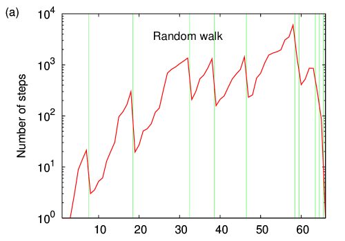
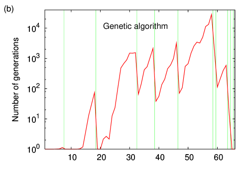
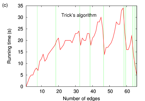
Figure 1: Performance of three algorithms to find the chromatic numbers of the graphs in $\mathcal{G}$: a random walker (a), a genetic algorithm (b), and Trick’s implementation [24] of the algorithm in [9] (c). The data shown for (a) are averages over $10\,000$ independent runs. The genetic algorithm is the one described in the caption to Fig. 15 in [4], parameter values included, and the data shown for (b) are averages over $100$ independent runs.

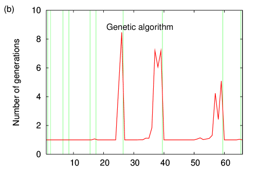
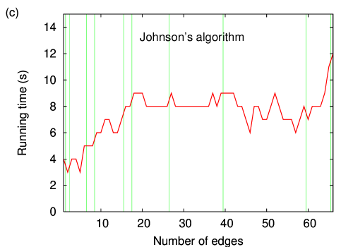
Figure 2: Performance of three algorithms to find the independence numbers of the graphs in $\mathcal{G}$: a random walker (a), a genetic algorithm (b), and Johnson’s implementation [16] of the algorithm in [10] (c). The data shown for (a) are averages over $10\,000$ independent runs. The genetic algorithm is the one described in the caption to Fig. 15 in [4], parameter values included, and the data shown for (b) are averages over $100$ independent runs.

Let us then look at one single sequence $\mathcal{G}=\langle G_{1},G_{2},\ldots,G_{M}\rangle$ for $n=12$ (whence $M=66$) and observe how different algorithms to find $\chi(G_{1}),\chi(G_{2}),\ldots,\allowbreak\chi(G_{M})$ and $\alpha(G_{1}),\alpha(G_{2}),\ldots,\alpha(G_{M})$ perform. Results on finding the chromatic numbers are given in Fig. 1; those on finding the independence numbers are in Fig. 2.

Figure 1 contains performance data on three algorithms. First is a simple random walker, which for each $m$ starts at a randomly chosen acyclic orientation in $\Omega_{m}$ and then at each step traverses one of the edges that outgo from its current acyclic orientation in the set $E_{m}$, thus reaching another acyclic orientation. Performance data are then given for a genetic algorithm operating on $\Omega_{m}$, and then for a deterministic algorithm whose operation is not based on $D_{m}$ at all. The random walker and the genetic algorithm stop upon hitting the first acyclic orientation $\omega$ for which $\mathrm{Depth}(\omega)=\chi(G_{m})$, with the provision that $\chi(G_{m})$ is known beforehand from running the third algorithm first. The data on all three algorithms are shown in the three parts of Fig. 1 against a backdrop of vertical lines, each marking the number of edges at which a transition in the chromatic number occurs: for $1\leq m<M$, if $\chi(G_{m+1})=\chi(G_{m})+1$, then a vertical line is drawn at the abscissa $m+0.5$. The chromatic numbers of the graphs in $\mathcal{G}$ necessarily increase by $1$ at each transition, from $\chi(G_{1})=2$ through $\chi(G_{M})=n$, therefore there are $n-2$ vertical lines all told.

A similar arrangement holds for Fig. 2, whose setting differs from that of the previous one in that now both the random walker and the genetic algorithm stop upon finding $\omega\in\Omega_{m}$ such that $\mathrm{Width}(\omega)=\alpha(G_{m})$, once again given that $\alpha(G_{m})$ is known a priori from running the deterministic algorithm first. There is also an important difference regarding the transitions in the graphs’ independence numbers, which now necessarily decrease by $1$ at each transition, from $\alpha(G_{1})=n-1$ through $\alpha(G_{M})=1$, thus totaling $n-2$ transitions as well. So, in Fig. 2, the vertical lines marking the transitions are drawn at the abscissae $m+0.5$ such that $\alpha(G_{m+1})=\alpha(G_{m})-1$.

Parts (a) and (b) of both Figs. 1 and 2 thus refer to methods which work on the sets $\Omega_{m}$ of acyclic orientations of the graphs $G_{m}$, either making explicit use of the structure of each $D_{m}$ (which the random walker does) or allowing for longer jumps as the orientations undergo the crossover and mutation operations prescribed by the genetic algorithm. The data displayed in the corresponding four panels often have in common the property that the occurrence of a transition, say from $m^{\prime}$ to $m^{\prime}+1$ edges, causes the algorithm in question to perform significantly better on $G_{m^{\prime}+1}$ than on $G_{m^{\prime}}$, and then increasingly poorly through the following values of $m$ until the next transition, if any, is reached. This difference in performance is sometimes quite marked, involving improvements by at least one order of magnitude.

What is perhaps more curious is that the same behavior is also present in Fig. 1(c), which refers to a deterministic algorithm to find chromatic numbers that does not rely on the $D_{m}$ graphs (in fact, this algorithm’s underlying strategy makes no reference at all to the acyclic orientations of the graph whose chromatic number it is seeking). Informally, then, this seems to indicate that the characteristic performance jumps at the transitions are inherent to the optimization problem itself (and only marginally, if at all, dependent upon how its feasible solutions are represented). It also seems to confer to the $D_{m}$ graphs some of the primitive representational character we sought in the beginning. However, Fig. 2(c), which also refers to a deterministic algorithm that does not operate on acyclic orientations, only now to find the graph’s independence number, shows none of the effects on performance at the transitions that the random-walk and genetic-algorithm approaches exhibit. The reason for this is that, despite being just as nominally NP-hard as the problem of finding chromatic numbers, finding independence numbers is easier in practice than that other problem. What this means is that, in order for the transitions’ effects on performance to show, substantially higher values of $n$ are needed (cf. Fig. 9 in [4]).

We then proceed on the premise that the sequence of $D_{m}$ graphs for $m=1,2,\ldots,M$ contains information enough to explain the performance jumps at the transitions, even though quantitatively we can only resort to what can be derived from each graph’s nodes’ depths, widths, and out-degrees. One initial indication that this makes sense comes from investigating the mutual information of pairs of random variables associated with each $D_{m}$. Given two discrete random variables and the joint distribution of their values, their mutual information is a measure of how much fixing the value of one of them reduces the uncertainty on the value of the other [18]. Just like Shannon’s entropy, mutual information is expressed in (information-theoretic) bits.

In the context of finding $\chi(G_{m})$, two discrete random variables of interest are those that give the out-degree and the depth of a randomly chosen node of $D_{m}$. Their joint distribution is $S_{m}(k,u)$ in the case of full degrees, $S_{m}^{B}(k,u)$ in the case of optimum-bound degrees, both introduced earlier. Their mutual information is, respectively for each case, given by

$$I_{m}=\sum_{k=1}^{m}\sum_{u=2}^{n}S_{m}(k,u)\log_{2}\frac{S_{m}(k,u)}{P_{m}(k)Q_{m}(u)}$$ (9)

and

$$I_{m}^{B}=\sum_{k=0}^{m}\sum_{u=2}^{n}S_{m}^{B}(k,u)\log_{2}\frac{S_{m}^{B}(k,u)}{P_{m}^{B}(k)Q_{m}^{B}(u)}.$$ (10)

If the problem is to find $\alpha(G_{m})$, then the two random variables give the node’s out-degree and its width. Their joint distributions are $T_{m}(k,v)$ and $T_{m}^{B}(k,v)$, once again depending on whether full or optimum-bound degrees are referred to. The respective measures of mutual information are

$$J_{m}=\sum_{k=1}^{m}\sum_{v=1}^{n-1}T_{m}(k,v)\log_{2}\frac{T_{m}(k,v)}{P_{m}(k)R_{m}(v)}$$ (11)

and

$$J_{m}^{B}=\sum_{k=0}^{m}\sum_{v=1}^{n-1}T_{m}^{B}(k,v)\log_{2}\frac{T_{m}^{B}(k,v)}{P_{m}^{B}(k)R_{m}^{B}(v)}.$$ (12)

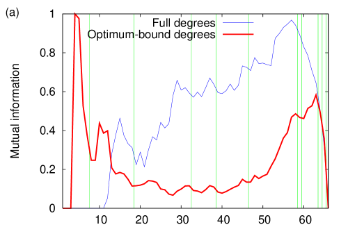
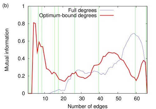
Figure 3: $I_{m}$ and $I_{m}^{B}$ (a); $J_{m}$ and $J_{m}^{B}$ (b). All data refer to the sequence $\mathcal{G}$.

For the same sequence $\mathcal{G}$ we have considered so far in this section, and following the same conventions as Figs. 1 and 2 with regard to marking with vertical lines the values of $m$ at which $\chi(G_{m})$ or $\alpha(G_{m})$ changes along the sequence, we show in Fig. 3 the progress of these four mutual information functions, in part (a) for graph coloring, in part (b) for independent sets. Note, in all cases, that although consistently less than one bit, all four functions are nearly always positive, thus providing evidence that, in most $D_{m}$ instances, out-degrees of either kind are independent from neither depths nor widths. However, the functions do not seem to behave consistently at the transitions and for this reason offer no direct explanation for what happens there.

It is important to recall that all of Figs. 1–3 refer to the one single sequence $\mathcal{G}$. They have been offered as illustrations of what is typical, and averaging over multiple graph sequences, which requires that we address the fact that a given transition may occur at different $m$ values in different sequences, might blur the reader’s understanding of what the phenomenon is and how mutual information suggests that it has to do with the $D_{m}$ graphs. We now turn to the role played by graph conduciveness and, after one more single-sequence illustration, do some averaging as properly as possible.

4 Computational results on conduciveness

Given a $D_{m}$ graph, let $\Omega_{m}^{\chi}$ denote the subset of $\Omega_{m}$ whose members are those of depth $\chi(G_{m})$. Analogously, let $\Omega_{m}^{\alpha}$ denote the subset of $\Omega_{m}$ whose members are those of width $\alpha(G_{m})$. We study four kinds of conduciveness of $D_{m}$, given as follows with reference to Eq. (1):

$$C_{m}^{\chi,\mathrm{in}} = \mathrm{Cond}_{\Omega_{m}\setminus\Omega_{m}^{\chi},\Omega_{m}^{\chi}}(D_{m});$$ (13)

$$C_{m}^{\chi,\mathrm{out}} = \mathrm{Cond}_{\Omega_{m}^{\chi},\Omega_{m}\setminus\Omega_{m}^{\chi}}(D_{m});$$ (14)

$$C_{m}^{\alpha,\mathrm{in}} = \mathrm{Cond}_{\Omega_{m}\setminus\Omega_{m}^{\alpha},\Omega_{m}^{\alpha}}(D_{m});$$ (15)

$$C_{m}^{\alpha,\mathrm{out}} = \mathrm{Cond}_{\Omega_{m}^{\alpha},\Omega_{m}\setminus\Omega_{m}^{\alpha}}(D_{m}).$$ (16)

Note that $C_{m}^{\chi,\mathrm{in}}$ is the conduciveness of $D_{m}$ from all orientations that are non-optimal for coloring to those that are optimal, $C_{m}^{\chi,\mathrm{out}}$ the conduciveness in the opposite direction. The situation with $C_{m}^{\alpha,\mathrm{in}}$ and $C_{m}^{\alpha,\mathrm{out}}$ is totally analogous, now regarding optimality for independent sets. We refer to $C_{m}^{\chi,\mathrm{in}}$ and $C_{m}^{\alpha,\mathrm{in}}$ as being inbound, to $C_{m}^{\chi,\mathrm{out}}$ and $C_{m}^{\alpha,\mathrm{out}}$ as being outbound. Note also that, by Eq. (1), and given the antiparallel nature of the edge set of $D_{m}$, it holds that

$$C_{m}^{\chi,\mathrm{out}}=\frac{\sum_{\omega\in\Omega_{m}\setminus\Omega_{m}^{\chi}}d_{\omega}}{\sum_{\omega\in\Omega_{m}^{\chi}}d_{\omega}}C_{m}^{\chi,\mathrm{in}}$$ (17)

and

$$C_{m}^{\alpha,\mathrm{out}}=\frac{\sum_{\omega\in\Omega_{m}\setminus\Omega_{m}^{\alpha}}d_{\omega}}{\sum_{\omega\in\Omega_{m}^{\alpha}}d_{\omega}}C_{m}^{\alpha,\mathrm{in}}.$$ (18)

These, however, imply no obvious relationship between the inbound conduciveness of $D_{m}$ and its outbound conduciveness for any of the two problems.

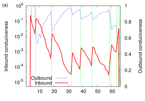
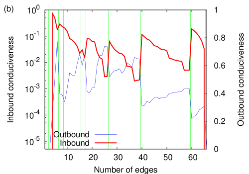
Figure 4: $C_{m}^{\chi,\mathrm{in}}$ and $C_{m}^{\chi,\mathrm{out}}$ (a); $C_{m}^{\alpha,\mathrm{in}}$ and $C_{m}^{\alpha,\mathrm{out}}$ (b). All data refer to the sequence $\mathcal{G}$.

An illustration of the kind of relationship that does hold is given in Fig. 4, which results from our last use of the same single sequence $\mathcal{G}$ as in the previous section. Strikingly, as the sequence unfolds with increasing $m$ and the transitions in $\chi(G_{m})$ [part (a) of the figure] or $\alpha(G_{m})$ [part (b) of the figure] occur, the inbound conduciveness of $D_{m}$ undergoes sudden jumps upwards precisely at the transitions while its outbound conduciveness undergoes downward jumps. The inbound-conduciveness jumps can be seen to encompass at least one order of magnitude in many cases. Between one transition and the next, the inbound conduciveness deteriorates progressively while the outbound conduciveness improves. This is then the key to interpreting the phenomena illustrated in Figs. 1 and 2: at the transitions, $D_{m}$ becomes markedly more conducive in the direction of the optimal orientations and less conducive in the opposite direction; right past a transition through right before the next one happens, $D_{m}$ tends to become progressively less conducive in the direction of the optima, more conducive in the direction that leads away from them.

Next we study these conduciveness variations as averages over the graph sequences $\mathcal{G}_{1},\mathcal{G}_{2},\ldots,\mathcal{G}_{15}$, each comprising graphs on $n=12$ nodes and generated independently. As noted earlier, even though both the chromatic number and the independence number undergo $n-2$ transitions each in each sequence, the $t$th transition, for some $t\in\{1,2,\ldots,n-2\}$, may happen at different values of $m$ for the different sequences. Some alignment of the transitions is then needed for the averages of interest to be computed; we proceed as follows. If for a given sequence the $t$th chromatic-number transition occurs for $m=m^{\prime}$, then we calculate the change ratios $(C_{m^{\prime}+1}^{\chi,\mathrm{in}}-C_{m^{\prime}}^{\chi,\mathrm{in}})/C_{m^{\prime}}^{\chi,\mathrm{in}}$ and $(C_{m^{\prime}+1}^{\chi,\mathrm{out}}-C_{m^{\prime}}^{\chi,\mathrm{out}})/C_{m^{\prime}}^{\chi,\mathrm{out}}$. We do likewise for each independence-number transition. If two subsequent chromatic-number transitions occur at $m=m^{\prime}$ and $m=m^{\prime\prime}>m^{\prime}$, then we also calculate the change ratios $(C_{m^{\prime\prime}}^{\chi,\mathrm{in}}-C_{m^{\prime}+1}^{\chi,\mathrm{in}})/C_{m^{\prime}+1}^{\chi,\mathrm{in}}$ and $(C_{m^{\prime\prime}}^{\chi,\mathrm{out}}-C_{m^{\prime}+1}^{\chi,\mathrm{out}})/C_{m^{\prime}+1}^{\chi,\mathrm{out}}$, again proceeding likewise for the interval between every pair of subsequent independence-number transitions. The latter formulae can also be used to calculate change ratios for the interval that precedes the first transition (letting $m^{\prime}=0$ and $m^{\prime\prime}$ be the value of $m$ at which the first transition occurs) and the interval that succeeds the last transition (letting $m^{\prime}$ be value of $m$ at which the last transition occurs and $m^{\prime\prime}=M$). Once all change ratios have been calculated, they can be averaged over the $15$ sequences for each transition (whichever the value of $m$ is at which it happens to occur in each sequence) and each interval.

These average change ratios are given in Figs. 5 and 6, respectively for graph coloring and independent sets. All data in these two figures are presented, as in all previous cases, against a backdrop of vertical lines. These, however, are now equally spaced and refer to the transition numbers, from $1$ through $n-2$, regardless of the $m$ values at which the transitions themselves are observed in each particular sequence for each problem. Each panel in each figure contains two plots, one with points whose abscissae coincide with those of the vertical lines (this refers to change ratios at the transitions) and one with points whose abscissae stand either halfway between those of two consecutive vertical lines or to the left (right) of the leftmost (rightmmost) vertical line’s abscissa [this refers to change ratios along the intervals between consecutive transitions or before (after) the first (last) transition].

Figs. 5(a) and 6(a), which refer to the progress of the inbound conduciveness as the transitions elapse, reveal that at most transitions the upward jumps represent significant fractions of the pre-transition conduciveness values, which often increase manyfold (by a factor of a few tens). On the other hand, the accumulated deterioration in conduciveness that is observed between transitions and in the outermost intervals is in most cases given by a fraction that varies widely depending on the transition, ranging practically from nearly no loss of the initial conduciveness inside the interval to nearly total loss.

Figs. 5(b) and 6(b), in turn, refer to how the outbound conduciveness values evolve along with the transitions and show that, right at the transitions, conduciveness is lost with respect to the pre-transition values by fractions that amount to losing from about $5$–$10$% of it (depending on the problem) to all of it. As we look at the accumulated improvement in conduciveness between transitions and in the outermost intervals, we see that a wide range of possibilities is again present, allowing at one extreme for practically no improvement and, at the other extreme, for an improvement by about $70$–$90$% of the initial conduciveness inside the interval (depending on the problem).

5 Summary and outlook

The notion of network conduciveness we have introduced is a simple degree-based indicator that can be interpreted as a probability with respect to a particular agent-related dynamics. We believe that, either as defined or as some variant thereof, it may find applications in network studies having to do with the dynamics of populations in networks. Our own application in this paper has been to the field of combinatorial optimization, and then the network in question is representative of the feasible solutions to a particular instance of an optimization problem and of how one may move from one solution to another through as simple a local transformation as possible. We tackled the NP-hard problems of finding an undirected graph’s chromatic and independence numbers and demonstrated how network conduciveness, when applied to problem representations in the domain of the graph’s acyclic orientations, is capable of helping explain the well-known performance transitions that occur along sequences of random graphs for both problems.

As it happens, though, the networks whose conduciveness we have considered grow very rapidly with the graph’s numbers of nodes and edges, and become themselves very nearly intractable already for small instances of the problems we addressed. We were then limited in our computational experiments to using graphs on $12$ nodes exclusively and to averaging results on $15$ sequences of random graphs. For the sake of the record, with current technology all experiments required nearly two months on twenty processors. So, as much as we think that there is great potential usefulness to the notion of a network’s conduciveness, further progress with the particular application we chose requires considerable further effort so that larger graphs and better statistical significance can be aimed at. On the other hand, we regard the first steps we have taken as very significant: to the best of our knowledge, no other study has addressed the intricacies of NP-hard optimization problems from the perspective of network theory applied to the structure that underlies the problems’ sets of feasible solutions.

Acknowledgments

We acknowledge partial support from CNPq, CAPES, and a FAPERJ BBP grant.

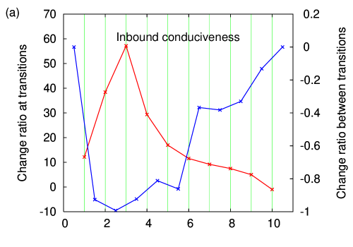
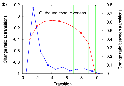
Figure 5: Conduciveness change ratios at the graph-coloring transitions and related intervals. Data are given as averages over the set of sequences $\mathcal{G}_{1},\mathcal{G}_{2},\ldots,\mathcal{G}_{15}$ for both the inbound conduciveness (a) and the outbound conduciveness (b).

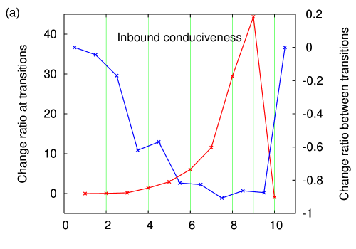
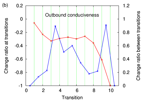
Figure 6: Conduciveness change ratios at the independent-set transitions and related intervals. Data are given as averages over the set of sequences $\mathcal{G}_{1},\mathcal{G}_{2},\ldots,\mathcal{G}_{15}$ for both the inbound conduciveness (a) and the outbound conduciveness (b).

References

- [1] V. C. Barbosa. An Atlas of Edge-Reversal Dynamics. Chapman & Hall/CRC, London, UK, 2000.
- [2] V. C. Barbosa, C. A. G. Assis, and J. O. do Nascimento. Two novel evolutionary formulations of the graph coloring problem. J. Comb. Optim., 8:41–63, 2004.
- [3] V. C. Barbosa and L. C. D. Campos. A novel evolutionary formulation of the maximum independent set problem. J. Comb. Optim., 8:419–437, 2004.
- [4] V. C. Barbosa and R. G. Ferreira. On the phase transitions of graph coloring and independent sets. Physica A, 343:401–423, 2004.
- [5] V. C. Barbosa and J. L. Szwarcfiter. Generating all the acyclic orientations of an undirected graph. Inform. Process. Lett., 72:71–74, 1999.
- [6] B. Bollobás, R. Kozma, and D. Miklós, editors. Handbook of Large-Scale Random Networks. Springer, Berlin, Germany, 2009.
- [7] J. A. Bondy and U. S. R. Murty. Graph Theory. Springer, New York, NY, 2008.
- [8] S. Bornholdt and H. G. Schuster, editors. Handbook of Graphs and Networks. Wiley-VCH, Weinheim, Germany, 2003.
- [9] D. Brélaz. New methods to color vertices of a graph. Commun. ACM, 22:251–256, 1979.
- [10] R. Carraghan and P. M. Pardalos. An exact algorithm for the maximum clique problem. Oper. Res. Lett., 9:375–382, 1990.
- [11] P. Cheeseman, B. Kanefsky, and W. M. Taylor. Where the really hard problems are. In Proceedings of the Twelfth International Joint Conference on Artificial Intelligence, pages 331–337, San Mateo, CA, 1991. Morgan Kaufmann Publishers.
- [12] J. Culberson and I. Gent. Frozen development in graph coloring. Theor. Comput. Sci., 265:227–264, 2001.
- [13] R. W. Deming. Acyclic orientations of a graph and chromatic and independence numbers. J. Comb. Theory B, 26:101–110, 1979.
- [14] M. R. Garey and D. S. Johnson. Computers and Intractability: A Guide to the Theory of NP-Completeness. W. H. Freeman, New York, NY, 1979.
- [15] A. Giordana and L. Saitta. Phase transitions in relational learning. Mach. Learn., 41:217–251, 2000.
- [16] D. S. Johnson. ftp://dimacs.rutgers.edu/pub/dsj/clique/dfmax.c.
- [17] D. S. Johnson. A catalog of complexity classes. In J. van Leeuwen, editor, Handbook of Theoretical Computer Science, volume A, pages 67–161. The MIT Press, Cambridge, MA, 1990.
- [18] P. E. Latham and Y. Roudi. Mutual information. Scholarpedia, 4(1):1658, 2009.
- [19] D. Mitchell, B. Selman, and H. Levesque. Hard and easy distributions of SAT problems. In Proceedings of the Tenth National Conference on Artificial Intelligence, pages 459–465, Menlo Park, CA, 1992. AAAI Press.
- [20] R. Monasson, R. Zecchina, S. Kirkpatrick, B. Selman, and L. Troyansky. Determining computational complexity from characteristic ‘phase transitions’. Nature, 400:133–137, 1999.
- [21] M. Newman, A.-L. Barabási, and D. J. Watts, editors. The Structure and Dynamics of Networks. Princeton University Press, Princeton, NJ, 2006.
- [22] J. Slaney and T. Walsh. Backbones in optimization and approximation. In Proceedings of the Seventeenth International Joint Conference on Artificial Intelligence, pages 254–259, San Francisco, CA, 2001. Morgan Kaufmann Publishers.
- [23] R. P. Stanley. Acyclic orientations of graphs. Discrete Math., 5:171–178, 1973.
- [24] M. A. Trick. http://mat.gsia.cmu.edu/COLOR/solvers/trick.c.