Quantum chaos and thermalization in gapped systems

Abstract

We investigate the onset of thermalization and quantum chaos in finite one-dimensional gapped systems of hard-core bosons. Integrability in these systems is broken by next-nearest-neighbor repulsive interactions, which also generate a superfluid to insulator transition. By employing full exact diagonalization, we study chaos indicators and few-body observables. We show that with increasing system size, chaotic behavior is seen over a broader range of parameters and, in particular, deeper into the insulating phase. Concomitantly, we observe that, as the system size increases, the eigenstate thermalization hypothesis extends its range of validity inside the insulating phase and is accompanied by the thermalization of the system.

The use of ultracold quantum gases to realize strongly correlated phases of matter has been at the forefront of research during the last decade Bloch et al. (2008). Such systems will not only help to understand phases and models introduced in the past, but also will create and will provide the means to investigate new exotic phases. Another major promise of the field is the possibility for studying the dynamics of correlated quantum systems in very controlled ways. For short times, the collapse and revival of phase coherence was analyzed in Ref. Greiner et al. (2002b) after an interaction quench from the Bose-Einstein condensate to the Mott insulating regime. Ab initio calculations of various bosonic and fermionic lattice models reproduced those observations Rigol et al. (2006); kollath07 ; manmana07 . A natural question that follows, given the fact that these systems are nearly isolated, is whether conventional statistical ensembles can describe experimental observables after relaxation.

Recent experiments have found that relaxation toward thermal equilibrium takes place in certain setups, but not in others Kinoshita et al. (2006). The lack of thermalization in the latter case can be associated with the proximity to integrability Rigol (2009a). At integrability, several works have shown that thermalization is not expected to occur Rigol et al. (2007), except for special conditions and/or observables Rigol et al. (2006); Rossini et al. (2009). For generic nonintegrable systems, thermalization is expected to occur and follows from the eigenstate thermalization hypothesis (ETH) Deutsch (1991); rigol08STATc .

Interestingly, in numerical calculations for quenches across a gapless to gapped phase, thermalization did not occur in the gapped side, even when the system was nonintegrable kollath07 . As a matter of fact, ETH, which was shown to hold in several nonintegrable gapless systems rigol08STATc ; Rigol (2009a), has been questioned for gapped systems Biroli et al. ; Roux . Questions raised include the proximity to the atomic limit, finite-size effects Roux , and the effects of rare states Biroli et al. within the insulating phase. Other studies that deal with spin and fermionic systems have found that relaxation toward equilibrium occurs faster close to a critical point Eckstein et al. (2009). The fact that, away from the ground state, these systems are, in general, not insulating, even if gaps are present in the spectrum, renders the debate more interesting still. Why then would generic nonintegrable gapped systems behave differently from gapless ones? Remarkably, in disordered systems, insulating behavior may take place away from the ground state huse , and those ones could indeed behave differently.

In this Rapid Communication, we use various measures, such as quantum chaos indicators Santos and Rigol and eigenstate expectation values of experimental observables Rigol (2009a) to understand whether thermalization should occur in gapped systems. This question is of interest for current experiments with ultracold gases, where systems with insulating ground states such as the bosonic and fermionic Mott insulators are studied. We show that thermalization does occur in the gapped side of the phase diagram and that, as the system size increases, thermalization is observed deeper into that phase. We also find that ETH holds for systems with larger gaps, as the system size is increased. This supports the view that thermalization occurs in generic nonintegrable systems independent of the presence or absence of gaps in the spectrum. One does need to be careful with temperature effects and finite-size effects, which may be more relevant close to integrable points Rigol (2009a) and in systems with gaps Roux . We also study the long-time dynamics of these gapped systems and address its universality.

We focus our study on the one-dimensional hard-core boson (HCB) model with nearest-neighbor hopping $t$, and nearest- and next-nearest-neighbor (NNN) interaction $V$ and $V^{\prime}$, respectively. The Hamiltonian is written as

$$\hat{H}_{b}=\sum_{i=1}^{L}\left\{-t\left(\hat{b}^{\dagger}_{i}\hat{b}_{i+1}+\textrm{H.c.}\right)\right.$$ (1)

$$+V\left.\left(\hat{n}^{b}_{i}-\dfrac{1}{2}\right)\left(\hat{n}^{b}_{i+1}-\dfrac{1}{2}\right)+V^{\prime}\left(\hat{n}^{b}_{i}-\dfrac{1}{2}\right)\left(\hat{n}^{b}_{i+2}-\dfrac{1}{2}\right)\right\}$$

where standard notation has been used Rigol (2009a). We restrict our analysis to lattices with 1/3 filling ($N_{b}=L/3$); $t=1$ sets the energy scale, $V=6$, and $V^{\prime}$ is varied ($0\leq V^{\prime}\leq 9$). For $V^{\prime}<V^{\prime}_{c}=3$, the ground state is a gapless superfluid, whereas for $V^{\prime}\geq V^{\prime}_{c}=3$, it is a gapped insulator Zhuravlev et al. (1997).

Eigenstate expectation values (EEVs) of different observables, as well as the nonequilibrium dynamics and thermodynamics of these systems, are determined using full exact diagonalization of the Hamiltonian in Eq. (1). We study lattices with up to 24 sites and 8 HCBs, which correspond to a total Hilbert space of dimension $D=735\,471$. We take advantage of the translational symmetry of the lattice to independently diagonalize each Hamiltonian block with total momentum $k$; the largest block in $k$ space has dimension $D_{k}=30\,667$ supplement .

The Hamiltonian in Eq. (1) is integrable when $V^{\prime}=0$, whereas the addition of NNN interaction leads to the onset of chaos. Note that the integrable-chaos transition may occur although random elements are nonexistent in the Hamiltonian Santos and Rigol . We start our study by addressing how quantum chaos indicators, such as level spacing distribution, level number variance, and inverse participation ratio (IPR) supplement , change as one moves away from the integrable point and eventually enter the gapped region by increasing $V^{\prime}$. The outcomes are shown to support our results on thermalization.

Level spacing distribution and level number variance are obtained from the unfolded spectrum of each $k$ sector separately. The first is a measure of short-range correlations, and the second is a measure of long-range correlations Guhr et al. (1998). For integrable systems, the distribution of spacings $s$ of neighboring energy levels may cross, and the distribution is Poissonian $P_{P}(s)=\exp(-s)$, while for nonintegrable systems, level repulsion leads to the Wigner-Dyson distribution. The form of the latter depends on the symmetries of the system. Here, it coincides with that of ensembles of random matrices with time reversal invariance, the so-called Gaussian orthogonal ensembles (GOEs): $P_{\text{GOE}}(s)=(\pi s/2)\exp(-\pi s^{2}/4)$. The level number variance is defined as $\Sigma^{2}(l)\equiv\langle N(l,\epsilon)^{2}\rangle-\langle N(l,\epsilon)\rangle^{2}$, where $N(l,\epsilon)$ is the number of states in the energy interval $[\epsilon,\epsilon+l]$ and $\langle.\rangle$ is the average over different initial values of $\epsilon$. For a Poisson distribution $\Sigma^{2}_{P}(l)=l$, while for GOEs in the limit of large $l$, $\Sigma^{2}_{\text{GOE}}(l)=2[\ln(2\pi l)+\gamma+1-\pi^{2}/8]/\pi^{2}$, where $\gamma$ is the Euler constant.

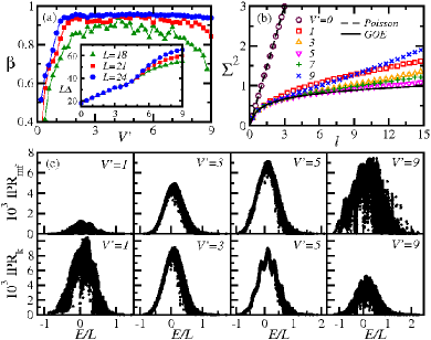
Figure 1: (Color online) (a) Parameter $\beta$ of the Brody distribution used to fit the average of the level spacing distributions over all sectors with $k=1,\ldots,\left\lfloor L/2\right\rfloor$. The inset shows the gap (between the lowest energy states) times $L$ vs $V^{\prime}$. (b) Level number variance averaged over the same $k$ sectors, for $L=24$, and compared to the Poisson and GOE results. (c) Inverse participation ratio in the mean-field (mf) (top) and momentum (bottom) basis vs energy per site; $L=24$, $k=2$, and $D_{k}=30\,624$.

Figures 1(a) and 1(b) show results for $P(s)$ and $\Sigma^{2}(l)$, respectively, for different values of $V^{\prime}$. The level spacing distribution is parametrized by $\beta$, which is used to fit $P(s)$ with the Brody distribution Brody et al. (1981), $P_{B}(s)=(\beta+1)bs^{\beta}\exp\left(-bs^{\beta+1}\right)$, where $b=\left[\Gamma\left(\frac{\beta+2}{\beta+1}\right)\right]^{\beta+1}$ supplement . Two transitions are verified: (i) from integrable [$\beta\rightarrow 0,\Sigma^{2}(l)\rightarrow l$] to chaotic [$\beta\rightarrow 1,\Sigma^{2}(l)\rightarrow\Sigma^{2}_{\text{GOE}}(l)$] as $V^{\prime}$ increases from $V^{\prime}=0$, and (ii) a departure from chaoticity for large values of $V^{\prime}$. Figure 1(a) also shows a strong dependence of the results on the system size. For larger systems, smaller values of $V^{\prime}$ suffice for the first integrable-chaos transition, and larger values of $V^{\prime}$ are required for the second transition. It is an open question whether, in the thermodynamic limit, any value of $V^{\prime}\neq 0$ would implicate chaoticity for these systems. However, for our finite systems, we do find an overlap between the gapped phase and the chaotic regime. The behavior of the gap $\Delta$ (times $L$) vs $V^{\prime}$ is depicted in the inset in Fig. 1(a). Notice the kink around $V^{\prime}_{c}\sim 3$, which signals the onset of the superfluid-insulator transition.

The IPR measures the level of delocalization of the eigenstates Izrailev (1990). Contrary to the two previous quantities, IPR depends on the basis chosen for the analysis. For an eigenstate $|\psi_{\alpha}\rangle$ of Eq. (1) written in the basis vectors $|\phi_{j}\rangle$ as $|\psi_{\alpha}\rangle=\sum_{j=1}^{D_{k}}c^{j}_{\alpha}|\phi_{j}\rangle$, we have $\mbox{IPR}_{\alpha}\equiv(\sum_{j=1}^{D_{k}}|c^{j}_{\alpha}|^{4})^{-1}$. In Fig. 1(c), we investigate IPR in two bases: the mf basis (IPR${}_{\text{mf}}$), where the $|\phi_{j}\rangle$’s are the eigenstates of the integrable Hamiltonian ($V^{\prime}=0$); and the $k$ basis (IPR_k), where the $|\phi_{j}\rangle$’s are the total momentum basis vectors. Small vs large values of IPR${}_{\text{mf}}$ separate regular from chaotic behavior Zelevinsky et al. (1996) and signal delocalization during the first integrable-chaos transition. The reduction of IPR_k indicates localization in $k$ space, which in our model, results from approaching the atomic limit in the presence of translational symmetry. Hence, it explains the departure from chaoticity for $V^{\prime}\gg V^{\prime}_{c}$ supplement .

The structures of the eigenstates are intimately connected to the thermalization process. As stated by the ETH, thermalization is expected to occur when the expectation values of experimental observables (with respect to eigenstates of the Hamiltonian that are close in energy) are very similar to each other and, hence, are equal to the microcanonical average, that is, thermalization occurs at the level of eigenstates. This is certainly the case with GOEs, where the amplitudes $c^{j}_{\alpha}$ for all $|\psi_{\alpha}\rangle$’s are independent random numbers. GOE eigenstates in any basis then lead to $\mbox{IPR}_{\text{GOE}}\sim D_{k}/3$ Zelevinsky et al. (1996). For our lattices, IPR${}_{\text{mf}}$ and IPR_k may approach the GOE value only in the middle of the spectrum, as expected for systems with finite-range interactions Kota (2001); Santos and Rigol . States at the edges, even in the chaotic limit, are more localized. In addition, as shown in the panels of Fig. 1(c), the values of IPRs for eigenstates close in energy fluctuate significantly as one moves away from the chaotic limit, namely, as $V^{\prime}\rightarrow 0$, where the system becomes localized in the mf basis, and for $V^{\prime}\gg V^{\prime}_{c}$, where the system becomes localized in the $k$ basis. Thus, ETH is not expected to hold in these regions. On the contrary, for intermediate values of $V^{\prime}$, IPR${}_{\text{mf}}$ and IPR_k become smooth functions of energy, especially for $E<0$. We may, therefore, anticipate compliance with the ETH even after the opening of the gap.

To verify the relation between ETH and the chaos measures analyzed previously, we have studied the EEVs of one- and two-body observables for different values of $V^{\prime}$ as one crosses the superfluid to insulator transition. We have found qualitatively similar results for them, so we only report here on the kinetic energy [$K=\sum_{i}-t\left(\hat{b}^{\dagger}_{i}\hat{b}_{i+1}+\textrm{H.c.}\right)$] and the momentum distribution function [$n(k)$]. Both are one-body observables, although the former one is local, while the latter is not. $K$ and $n(k)$ are routinely measured in cold gases experiments.

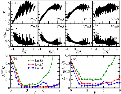
Figure 2: (Color online) (a) EEVs of $K$ (top) and $n(k)$ (bottom) vs energy per site for the full spectrum (which include all momentum sectors). Results are shown for four different values of $V^{\prime}$ and $L=24$. Panels (b) and (c) average relative deviation of the EEVs of (b) $K$ and (c) $n(k=0)$ with respect to the microcanonical result vs $V^{\prime}$, for $T=3$ (see text) and three different lattice sizes. $T=3$ ($L=24$) corresponds to $E=-10.7$ for $V^{\prime}=1$, $E=-10.0$ for $V^{\prime}=3$, $E=-11.7$ for $V^{\prime}=5$, and $E=-19.3$ for $V^{\prime}=9$.

Figure 2(a) depicts the EEVs of $K$ and $n(k)$ for all eigenstates of the Hamiltonian and for different values of $V^{\prime}$. For small values of $V^{\prime}$ ($V^{\prime}<2$ for $L=24$), there are large fluctuations of the EEVs of both observables over the entire spectrum. As $V^{\prime}$ increases and one departs from integrability, these fluctuations reduce in the center of the spectrum, and ETH becomes valid. To increase $V^{\prime}$ even further (beyond the superfluid to insulator transition), increases the fluctuations of the EEVs once again as the eigenstates begin to localize in $k$ space. These results are in clear agreement with what we expected based on the chaos indicators supplement .

To be more quantitative, we study the average deviation of the EEVs with respect to the microcanonical result ($\Delta^{mic}$). For an observable $O$, we define $\Delta^{mic}O=(\sum_{\alpha}\,|O_{\alpha\alpha}-O_{mic}|)/(\sum_{\alpha}\,O_{\alpha\alpha})$, where the sum is performed over the microcanonical window and $O_{\alpha\alpha}$ are the EEVs of $\hat{O}$. The microcanonical expectation values are computed as usual. We average over all eigenstates (from all momentum sectors) that lie within a window $[E-\Delta E,E+\Delta E]$, and take $\Delta E=0.1$. We have checked that our results are independent of the exact value of $\Delta E$ in the neighborhood of $\Delta E=0.1$. Here, we select $E$ such that, for different values of $V^{\prime}$, the effective temperature ($T=3$) is the same for all systems sizes temperature .

Results for $\Delta^{mic}K$ and $\Delta^{mic}n(k=0)$ are presented in Figs. 2(b) and 2(c) supplement . They show that, in general, as the system size increases: (i) The average deviations of both observables decrease, and (ii) the upturn that occurs as localization starts to set in $k$ space moves toward larger values of $V^{\prime}$. A comparison between the lower and upper panels in Fig. 2 also shows that where $\Delta^{mic}K$ and $\Delta^{mic}n(k=0)$ are minimal, so are the maximal fluctuations of $K$ and $n(k=0)$ in the individual eigenstates, and they decrease with increasing systems size supplement . Hence, ETH is valid in that regime and we find no evidence of rare states Biroli et al. . The above results are in agreement with the chaos measure predictions and indicate that, for thermodynamic systems, ETH may be valid, away from the edges of the spectrum, even if one is deep into the insulating side of the phase diagram.

Equipped with this knowledge, we are now ready to study the dynamics of such systems after a quench. Our initial states are always selected from the eigenstates of (1) with $t=1$, $V=6$, $V^{\prime}_{ini}$ and zero total momentum, and then we quench $V^{\prime}_{ini}\rightarrow V^{\prime}$. After a systematic analysis, we have found that the short-time dynamics depends strongly on the initial state and the final Hamiltonian, so we will focus here on the long-time dynamics and the outcome of relaxation. As discussed previously manmana07 ; Rigol (2009a); rigol08STATc , after relaxation, observables are well described by the diagonal ensemble $O_{diag}=\sum_{\alpha}|C_{\alpha}|^{2}O_{\alpha\alpha}$, where $C_{\alpha}$ is the overlap of the initial state with eigenstate $\alpha$ of the Hamiltonian.

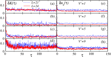
Figure 3: (Color online) Dynamics of the normalized difference between the evolving expectation values of $K$ (left panels) and $n(k)$ (right panels) and the diagonal ensemble prediction. Average over the evolution of nine initial states selected from the eigenstates of the Hamiltonian with $V^{\prime}_{ini}=0,1,\ldots,9$ (excluding the $V^{\prime}$ used for the dynamics). The nine states for each $V^{\prime}$ were chosen such that the (conserved) energies during the time evolution are the same in all cases, and $T=3$. Given the energy of the initial state in the final Hamiltonian $E=\langle\psi_{ini}|\widehat{H}|\psi_{ini}\rangle$, $T$ is computed by following Ref. temperature .

In Fig. 3, we show the normalized difference between the time-evolving expectation value of $K$ and $n(k)$ and the diagonal ensemble prediction $\delta K$ (left panels) and $\delta n_{k}$ (right panels), respectively. We define $\delta K(\tau)=|K(\tau)-K_{diag}|/|K_{diag}|$ and $\delta n_{k}(\tau)=(\sum_{k}|n(k,\tau)-n_{diag}(k)|)/(\sum_{k}n_{diag}(k))$. In order to verify the universality of our results, for each value of $V^{\prime}$ used for the dynamics, we prepared nine initial states selected from the eigenstates of the Hamiltonian with different values of $V^{\prime}_{ini}$ (excluding $V^{\prime}$) and studied the dynamics for all of them. The long time dynamics was found to be very similar, independent of the initial state. In Fig. 3, we depict the average over those nine different time evolutions supplement . These plots show that after long times, observables relax to values similar to those predicted by the diagonal ensemble, and those predictions become more accurate with increasing system size. Only for $V^{\prime}=9$ do we find large time fluctuations of $K$, which is a consequence of the approach to localization in $k$ space. However, even these time fluctuations decrease with increasing system size.

Once it is known that the relaxation dynamics brings observables to the values predicted by the diagonal ensemble, and that the accuracy of that prediction improves with increasing system size, all we need to do to check whether the system thermalizes or not is to compare the predictions of the diagonal ensemble with the microcanonical ones. For larger systems, one could also compare with the canonical ensemble, but this is not adequate here due to finite-size effects Rigol (2009a).

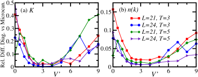
Figure 4: (Color online) Relative differences between the predictions of the microcanonical and diagonal ensembles for (a) $K$ and (b) $n(k)$ vs $V^{\prime}$, for $T=3.0$ and $T=5.0$. Results are shown for $L=21$, $N_{b}=7$ and $L=24$, $N_{b}=8$. The diagonal ensembles correspond to the quenches from the nine $V^{\prime}_{ini}$ of Fig. 3 to $V^{\prime}$, and the curves are averages over the nine relative differences. Relative differences are computed in exactly the same way as $\delta K$ and $\delta n_{k}$ in Fig. 3.

In Fig. 4, we depict the comparison between diagonal and microcanonical ensembles. Results are shown for the same set of quenches and initial states presented in Fig. 3, and for an additional set of initial states such that the effective temperature of the relaxed systems is a bit higher, namely, $T=5$ supplement . The results for $T=3$ and $T=5$ are in qualitative agreement with each other for our two observables of interest. They show that the microcanonical ensemble predicts the outcome of the relaxation dynamics with high accuracy for the intermediate values of $V^{\prime}$, where ETH was shown to be valid (cf. Fig. 2) and where quantum chaos was seen to emerge (cf. Fig. 1). It also shows that (i) the predictions of the microcanonical ensemble become more accurate with increasing system size, and (ii) the increasing disagreement between the microcanonical prediction and the outcome of the relaxation dynamics, after crossing the superfluid to insulator transition, moves to larger values of $V^{\prime}$ as the system size increases.

To summarize, our studies indicate that thermalization does occur in gapped systems. If integrability is broken, ETH was shown to be valid, away from the edges of the spectrum, even if gaps are present in the spectrum and the ground state of the system is an insulator. We verified that ETH holds where quantum chaos develops and that thermalization closely follows the validity of ETH (i.e., we found no instance where the rare event scenario put forward in Ref. Biroli et al. emerges in these systems). Our analysis of different lattice sizes showed that: (i) The range of parameters over which ETH applies increases with increasing system size; in particular, ETH becomes valid deeper into the insulating side of the phase diagram, and (ii) away from integrability, the fluctuations of the eigenstate expectation values of few-body observables decrease with increasing systems size. Further studies are needed to understand the dependence of the short-time dynamics on the initial state as well as the final Hamiltonian, and to determine the precise scaling, with system size, for the onset of ETH and quantum chaos.

I Hamiltonian and gapless-gapped transition

We study the one-dimensional hard-core boson (HCB) model with nearest-neighbor (NN) hopping $t$, and nearest- and next-nearest-neighbor (NNN) interaction $V$ and $V^{\prime}$, respectively. The Hamiltonian is written as

$$\hat{H}_{b}=\sum_{i=1}^{L}\left\{-t\left(\hat{b}^{\dagger}_{i}\hat{b}_{i+1}+\textrm{H.c.}\right)\right.$$ (2)

$$+V\left.\left(\hat{n}^{b}_{i}-\dfrac{1}{2}\right)\left(\hat{n}^{b}_{i+1}-\dfrac{1}{2}\right)+V^{\prime}\left(\hat{n}^{b}_{i}-\dfrac{1}{2}\right)\left(\hat{n}^{b}_{i+2}-\dfrac{1}{2}\right)\right\}.$$

Above, we take $\hbar=1$, $L$ is the size of the chain, $\hat{b}_{i}$ ($\hat{b}_{i}^{\dagger}$ ) is the bosonic annihilation (creation) operator on site $i$ and $\hat{n}_{i}^{b}=\hat{b}_{i}^{\dagger}\hat{b}_{i}$ is the boson local density operator. HCBs do not occupy the same site, so $b_{i}^{2}=b_{i}^{\dagger 2}=0$.

Hamiltonian (2) conserves the total number of particles $N_{b}$ and is translational invariant; it is then composed of independent blocks each associated with a value of $N_{b}$ and a total momentum $k$. Here we select $N_{b}=L/3$ and study all values of $k$, from 0 to $\ldots\left\lfloor L/2\right\rfloor$. Lattices with up to 24 sites and 8 HCBs are considered, corresponding to a total Hilbert space of dimension $D=735\,471$. The dimension $D_{k}$ of each $k$-sector is given in Table 1. We perform a full exact diagonalization of each sector independently.

Table 1: Dimension of subspaces

$L=18$	$k=0,6$	$k=1,5,7$	$k=2,4,8$	$k=3,9$
$D_{k}$	1038	1026	1035	1028
$L=21$	$k=0,7$	all other $k$’s
$D_{k}$	5538	5537
$L=24$	$k=0,8$	odd $k$’s	$k=2,6,10$	$k=4$
$D_{k}$	30667	30624	30664	30666

In what follows, $t=1$ sets the energy scale and we only consider repulsive interactions $V,V^{\prime}>0$. We fix $V=6$ and vary $V^{\prime}$ from 0 to 9. The system is integrable when $V^{\prime}=0$, while the addition of NNN interaction may lead to the onset of chaos. In addition, there is a critical value of the NNN interaction, $V^{\prime}_{c}=3$, below which the ground state is a gapless superfluid and above which it becomes a gapped insulator (see Ref. [17] in main text).

II Quantum Chaos Indicators

To analyze the transition from integrability to chaos, we study chaos indicators that depend only on the eigenvalues of the system, such as level spacing distribution and level number variance, and indicators that measure the level of delocalization of the eigenvectors, such as the inverse participation ratio (IPR) and the information (Shannon) entropy (S).

II.1 Level spacing distribution and level number variance

Level spacing distribution and level number variance give information about short-range and long-range correlations, respectively. They are obtained from the unfolded spectrum of each symmetry sector separately. The procedure of unfolding consists of locally rescaling the energies, so that the mean level density of the new sequence of energies is 1.

For integrable systems, the distribution of spacings $s$ of neighboring energy levels may cross and the distribution is Poissonian,

$$P_{P}(s)=\exp(-s),$$

whereas in nonintegrable systems, level repulsion leads to the Wigner-Dyson distribution. The form of the latter depends on the symmetries of the system. Hamiltonian (2) is time-reversal and rotationally invariant, it therefore gives the same distribution as random matrices with real and symmetric elements, the so-called Gaussian Orthogonal Ensembles (GOEs):

$$P_{\text{GOE}}(s)=\frac{\pi s}{2}\exp\left(-\frac{\pi s^{2}}{4}\right).$$

The level number variance is defined as

$$\Sigma^{2}(l)\equiv\langle(N(l,\epsilon)^{2}\rangle-\langle N(l,\epsilon)\rangle^{2},$$

where $N(l,\epsilon)$ is the number of states in the energy interval $[\epsilon,\epsilon+l]$ and $\langle.\rangle$ is the average over different initial values of the energy level $\epsilon$. For a Poisson distribution,

$$\Sigma^{2}_{P}(l)=l,$$

while for GOEs in the limit of large $l$,

$$\Sigma^{2}_{\text{GOE}}(l)=\frac{2}{\pi^{2}}\left[\ln(2\pi l)+\gamma+1-\frac{\pi^{2}}{8}\right],$$

where $\gamma$ is the Euler constant.

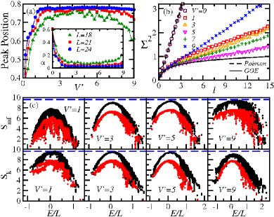
Figure 5: (Color online) (a) Peak position of the level spacing distribution averaged over all sectors with $k=1,\ldots,\left\lfloor L/2\right\rfloor$. The inset shows the quantity $\alpha$ (see text). (b) Level number variance averaged over the same $k$-sectors, for $L=21$, and compared to the Poisson and GOE results. (c) Shannon entropy in the mean-field (top) and momentum (bottom) basis vs energy per site; $k=2$; black: $L=24$, red: $L=21$; dashed line: S${}_{\text{GOE}}\approx 9.5969$ for $D_{2}=30\,664$.

Results for level spacing distribution and level number variance for various values of $V^{\prime}$ are shown in Figs. 5(a) and 5(b). These figures are equivalent to Figs. 1(a) and 1(b) in the main text. Note that because parity is a symmetry found only in the sector with $k=0$, this subspace is not included in the averages for both figures.

In Fig. 1(a) of the main text we quantified the integrable-chaos transition in terms of the parameter $\beta$ of the Brody distribution. In Fig. 5(a) we consider the peak position of the distribution, which shifts from zero to $\approx 0.7979$ during the crossover from $P_{P}(s)$ to $P_{WD}(s)$, and a quantity $\alpha$ (inset) defined as

$$\alpha\equiv\frac{\sum_{i}|P(s_{i})-P_{WD}(s_{i})|}{\sum_{i}P_{WD}(s_{i})}.$$ (3)

Above the sum runs over the whole spectrum. In the chaotic limit $\alpha\rightarrow 0$.

Figures 5(a) and 5(b) reinforce the main results of Figs. 1(a) and 1(b) in the main text, which are: (i) Two transitions are seen, from integrability to chaos as $V^{\prime}$ increases from $V^{\prime}=0$, and a departure from chaoticity for large values of $V^{\prime}$. (ii) By comparing the values of $V^{\prime}$ that induce chaos with the $V^{\prime}$ for the superfluid-insulator transition in the inset of Fig. 1(a), a region of overlap between the gapped phase and the chaotic regime is identified. (iii) A direct dependence exists between the system size and the width of the interval of $V^{\prime}$ values that lead to chaos; for larger systems the chaotic behavior goes deeper into the insulating phase. Larger system sizes bring also better agreement with the GOE results, as seen by comparing Fig. 1(b) in the main text, which was obtained for 24 sites, with Fig. 5(b), which deals with $L=21$.

II.2 Delocalization Measures

Delocalization measures, such as IPR and S, quantify the level of complexity of the eigenvectors (see references in main text). In general, they depend on the basis in which the computations are performed. For an eigenstate $|\psi_{\alpha}\rangle$ of Hamiltonian (2) written in the basis vectors $|\phi_{j}\rangle$ as $|\psi_{\alpha}\rangle=\sum_{j=1}^{D_{k}}c^{j}_{\alpha}|\phi_{j}\rangle$, IPR and S are respectively given by

$$\mbox{IPR}_{\alpha}\equiv\left(\sum_{j=1}^{D_{k}}|c^{j}_{\alpha}|^{4}\right)^{-1}$$

and

$$\mbox{S}_{\alpha}\equiv-\sum_{j=1}^{D_{k}}|c^{j}_{\alpha}|^{2}\ln|c^{j}_{\alpha}|^{2}.$$

These quantities indicate how much spread each $|\psi_{\alpha}\rangle$ is in the selected basis.

In the case of GOEs, the eigenvectors do not depend on the basis. They are simply random vectors, which give $\mbox{IPR}_{\text{GOE}}\sim D_{k}/3$ and $\mbox{S}_{\text{GOE}}\sim\ln(0.48D_{k})$. An essential difference of our system with respect to GOEs, besides the absence of randomness on it, is that Hamiltonian (2) has only two-body interactions. Consequently, its eigenstates may approach the GOE results only in the middle of the spectrum, close to the edges chaos does not fully develop.

In Fig. 5(c), we show S for two system sizes and in two bases. In the mean-field (mf) basis, $|\phi_{j}\rangle$’s correspond to the eigenstates of the integrable Hamiltonian ($V^{\prime}=0$); this choice separates regular from chaotic behavior. In the $k$-basis, $|\phi_{j}\rangle$’s are the basis vectors of total momentum. As $V^{\prime}$ increases from zero and the system undergoes the first transition, from integrability to chaos, the values of S${}_{\text{mf}}$ become larger, indicating delocalization of the eigenvectors in the mf-basis. The second transition, signaling the departure from chaoticity, is followed by the reduction of the values of S_k and the consequent localization of the eigenvectors in the $k$-basis. Even though the shrinking of the eigenvectors in $k$-space is better visualized in terms of IPR (main text), it is important to observe again that, similarly to the distancing of the eigenvalues from $P_{WD}(s)$ and $\Sigma^{2}_{\text{GOE}}(l)$, this localization occurs when $V^{\prime}$ is already beyond the critical point $V^{\prime}_{c}$ for the gapless-gapped transition.

The structure of the eigenstates gives us information about what to expect in terms of thermalization. The eigenstate thermalization hypothesis (ETH) states that thermalization should happen when the eigenstate expectation values (EEVs) do not fluctuate for states which are close in energy. In this case, the EEVs will equal the microcanonical average. The validity of ETH is therefore certain to hold for GOEs, where all eigenstates are extended and have the same level of complexity. For our two-body interaction system, two aspects must be taken into account: chaoticity and the energy of the initial state. Away from the chaotic regime, that is when $V^{\prime}\rightarrow 0$ or $V^{\prime}\gg V^{\prime}_{c}$, the structure of eigenstates close in energy fluctuate significantly, as shown by the panels of Fig. 5(c). But even in the chaotic region, fluctuations are seen also at the edges of the spectrum. Thus, thermalization in our lattice should occur in the chaotic domain and for initial states with energy away from the spectrum borders. This conclusion is the same we arrived at in Ref. [16] (main text), where we studied systems whose ground state was always gapless; therefore, as expected, the superfluid-insulator transition (a quantum phase transition) does not appear to affect the level of complexity of the bulk states. We note, however, that the results of the delocalization measures for system (2) show an asymmetry with respect to the middle of the spectrum that was not so evident in the systems of Ref. [16] (cf. Fig. 1(c), Fig. 5(c), and Figs.11-16 from Ref. [16]). In the present lattice, larger fluctuations in the values of S and IPR are present for $E>0$ for all values of $V^{\prime}$ studied.

III Eigenstate Thermalization Hypothesis

The connection between the ETH and the chaos indicators is reinforced by comparing the outcomes for the delocalization measures with those for the EEVs.

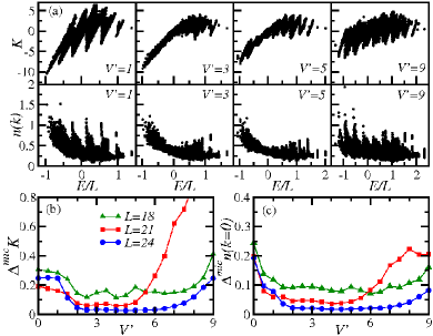
Figure 6: (Color online) (a) Eigenstate expectation values (EEVs) of $K$ (top) and $n(k)$ (bottom) vs energy per site for the full spectrum (including all momentum sectors). Results are shown for four different values of $V^{\prime}$ and $L=21$. Panels (b) and (c) correspond to the average relative deviation of the EEVs of $K$ (b) and $n(k=0)$ (c) with respect to the microcanonical result vs $V^{\prime}$ for $T=5$ (see text) and three different lattice sizes. $T=5$ ($L=24$) corresponds to $E=-6.24$ for $V^{\prime}=1$, $E=-5.55$ for $V^{\prime}=3$, $E=-6.61$ for $V^{\prime}=5$, and $E=-12.68$ for $V^{\prime}=9$.

The top and bottom panels of Fig. 6(a) show, respectively, the EEVS of the kinetic energy

$$\hat{K}=\sum_{i}-t\left(\hat{b}^{\dagger}_{i}\hat{b}_{i+1}+\textrm{H.c.}\right)$$

and the momentum distribution function

$$\hat{n}(k)=\frac{1}{L}\sum_{i,j}e^{-ik(i-j)}\hat{b}_{i}^{\dagger}\hat{b}_{j}$$

for all eigenstates. Fig. 6(a) is analogous to Fig. 2(a), but refers to a smaller system. The results in both figures mirror the behavior of the delocalization measures throughout the transitions. Large fluctuations of the EEVs are seen over the entire spectrum when the system is away from the chaotic limit, that is, when it approaches integrability and when it approaches localization in $k$-space. When chaos sets in, the fluctuations decrease mainly in the center of the spectrum, where the ETH is expected to be valid. We also should stress that, by comparing Fig. 6(a) with Fig. 2(a) in the chaotic regime, one can see that the fluctuations of the observables in all individual eigenstates (away from the edges of the spectrum) decrease with increasing systems size. This is a clear indication that the rare state scenario introduced in Ref. [13] in the main text does not take place in these systems.

To quantify the deviation of the EEV for an observable $O$ with respect to the microcanonical result ($\Delta^{mic}$), we define

$$\Delta^{mic}O\equiv\frac{\sum_{\alpha}\,|O_{\alpha\alpha}-O_{mic}|}{\sum_{\alpha}\,O_{\alpha\alpha}}.$$

Above, the sum runs over the microcanonical window, $O_{\alpha\alpha}$ are the EEVs of the operator $\hat{O}$, and the microcanonical expectation values $O_{mic}$ are computed as usual.

Figures 6(b) and 6(c) show the relative deviation $\Delta^{mic}K$ and $\Delta^{mic}n(k=0)$ averaged over all momentum sectors and for all eigenstates that lie within a window $[E-\Delta E,E+\Delta E]$, where $\Delta E=0.1$. We select $E$ according to the effective temperature $T$ that we want to study [$T=5$ here and $T=3$ in the equivalent Figs. 2(b) and 2(c) in the main text]. The analysis in terms of a single temperature allows for a fair comparison of all systems sizes and values of $V^{\prime}$. Temperature and energy are related by the expression

$$E=\dfrac{1}{Z}\textrm{Tr}\left\{\hat{H}e^{-\hat{H}/{k_{B}T}}\right\},$$ (4)

where $Z=\textrm{Tr}\left\{e^{-\hat{H}/{k_{B}T}}\right\}$ is the partition function, and we set $k_{B}$ to unity.

The results for $\Delta^{mic}K$ and $\Delta^{mic}n(k=0)$ for any given systems size comply with the predictions of chaos measures. As the system size increases, the average deviations for both observables decrease and the width of the interval of values of $V^{\prime}$ for which the EEVs approach the thermal average increases. We should add that for some specific values of $V^{\prime}$, the relative deviations are seen to be larger in some larger system sizes, that is, the curves in Fig. 6 and Fig. 2 in the main text cross. As we show next, this is a finite size effect related to bands of eigenvalues that move, within the temperature scale considered in this work, as the system size is changed.

IV Fluctuation of the EEV’s as a function of temperature

The study of the fluctuation of the EEV’s as a function of temperature gives further support to the discussions above.

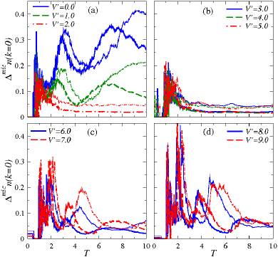
Figure 7: (Color online) Average relative deviation of eigenstate expectation values with respect to the microcanonical prediction as a function of the effective temperature $T$ of the eigenstates. Results for $\Delta^{mic}n(k=0)$ are given for the nine values of $V^{\prime}$ indicated and for systems with $L=24$ (thick lines) and $L=21$ (thin lines).

In Fig. 7, we present results for $\Delta^{mic}n(k=0)$ vs $T$ for nine different values of $V^{\prime}$ for systems with 24 and 21 lattice sites and $T\leq 10$. As before, distinct features are associated with different regimes. Far from chaoticity, large values of $\Delta^{mic}n(k=0)$ appear for all temperatures considered. In the chaotic domain, on the other hand, large values of $\Delta^{mic}n(k=0)$ are restricted to low temperatures, while at large $T$, $\Delta^{mic}n(k=0)$ saturates at small values. This corroborates our statements that the validity of ETH for these finite systems goes hand in hand with the onset of chaos and holds away from the edges of the spectrum.

In general, we also observe that larger systems reduce the average relative deviations. However, especially away from chaoticity, this rule may not be obeyed for particular values of the effective temperature and particular values of $V^{\prime}$. Notice in Fig. 7 the peaks with large fluctuations that move within our temperature scale as the system size is increased. These are responsible for the bumps seen in Figs. 2(b) and 2(c) in the main text and for the behavior of the fluctuations of the system with $L=21$ in Figs. 6(b) and 6(c). From the behavior seen here with increasing systems size, we expect them to disappear for very large system sizes.

V Long-Time Dynamics after a Quantum Quench

The endorsement of the predictions for thermalization drawn from chaos measures and the ETH is done in two steps. First we study the relaxation dynamics of the system to verify that it brings the observables $O$ close to the values of the diagonal ensemble,

$$O_{diag}=\sum_{\alpha}|C_{\alpha}|^{2}O_{\alpha\alpha},$$

where $C_{\alpha}$ is the overlap of the initial state $|\Psi(0)\rangle$ with the eigenstate $\alpha$ of the Hamiltonian, $C_{\alpha}=\langle\psi_{\alpha}|\Psi(0)\rangle$. Then we compare the results for the diagonal ensemble with those for the microcanonical ensemble. When they coincide we say that thermalization has taken place.

In the main text, the second step was presented in Fig. 4 for two values of temperature, $T=3$ and $T=5$. The relative differences between the predictions of the microcanonical and diagonal ensembles for $K$ and $n(k)$ became indeed small for values of $V^{\prime}$ where the ETH was shown to be valid. The first step was illustrated in Fig. 3 for $T=3$ and, for completeness, we now demonstrate that similar results hold for the dynamics of systems for which the effective temperature is $T=5$.

Figure 8: (Color online) Dynamics of the normalized difference between the evolving expectation values of $K$ (left panels) and $n(k)$ (right panels) and the diagonal ensemble prediction. The plots are the result of the average over the evolution of nine initial states selected from the eigenstates of the Hamiltonian with $V^{\prime}_{ini}=0,1,\ldots,9$ (excluding the $V^{\prime}$ used for the dynamics). The nine states for each $V^{\prime}$ were chosen such that the (conserved) energies during the time evolution are the same in all cases, and the effective temperature $T=5$. Given the energy of the initial state in the final Hamiltonian $E=\langle\psi_{ini}|\widehat{H}|\psi_{ini}\rangle$, the effective temperature is computed following Eq. (4).

Figure 8 gives the normalized difference between the time evolving expectation value of $K$ and $n(k)$ and the diagonal ensemble prediction, $\delta K$ (left panels) and $\delta n_{k}$ (right panels), respectively. We define $\delta K(\tau)=|K(\tau)-K_{diag}|/|K_{diag}|$ and $\delta n_{k}(\tau)=(\sum_{k}|n(k,\tau)-n_{diag}(k)|)/(\sum_{k}n_{diag}(k))$. For each value of $V^{\prime}$ considered in the analysis of the dynamics, nine initial states, all corresponding to $T=5$, were selected from the eigenstates of the Hamiltonian with different values of $V^{\prime}_{ini}$ (excluding $V^{\prime}$). We studied the evolution of the nine states after the quench and verified that their long-time dynamics were very similar. In Fig. 8, we display the average over those nine different time evolutions. The plots show that after long times, observables relax to values similar to those predicted by the diagonal ensemble and those predictions become more accurate with increasing system size. Only for $V^{\prime}=9$ we find large time fluctuations of $K$ and a much longer time scale for relaxation, which is a consequence of the approach to localization in $k$-space. However, even in the latter case, the time fluctuations are always seen to decrease with increasing system size.