Precision measurement of Higgs decay branching ratios to bottom quarks and gluons at the ILC

Abstract

The measurement of hadronic Higgs Boson branching ratios H$\rightarrow b\bar{b}$, H$\rightarrow gg$ for a light Standard Model-like Higgs boson produced at 250 GeV centre of mass energy at the International Linear Collider (ILC) is presented. The tools and techniques used for the analysis are briefly discussed.

1 Introduction

The measurement of Higgs boson branching ratios is one of the main features of the International Linear Collider (ILC) program [1]. For Higgs masses below 140 GeV, hadronic branching ratios can be precisely measured at the ILC. The final states have significant rates and the micro-vertex detector allows for good flavour identification. This measurement of relative couplings of the Higgs boson to fermions will allow to confirm the prediction of the Higgs mechanism that they are proportional to fermion masses. The branching fraction to b and c quarks is larger than the branching fraction to light quarks due to the mass. The Higgs decay to gluons in the Standard Model is mediated by heavy quark loops as shown in Figure 1. The branching ratio to gluons is indirectly related to $t\bar{t}$H Yukawa coupling [2] and would probe the existence of new strongly interacting particles that couple to the Higgs and are too heavy to be produced directly.

Figure 1: Higgs decay to gluons mediated by a heavy quark loop.

In this study we consider Higgs decays to bottom quarks and gluons in two- and four-jet configurations. For a $m_{H}$ = 120 GeV SM Higgs boson, we expect BR(H $\rightarrow b\bar{b}$) = 67.92% and BR(H $\rightarrow gg$) = 7.06% [3]. These decay modes exercise the tagging of heavy and light quarks [4, 5].

2 Analysis

The analysis strategy closely follows the one implemented in  [4].

2.1 Event Generation and Detector Simulation

In this study, the signal sample includes a Higgs boson produced in the Higgs-strahlung process, $e^{+}e^{-}{\to}$ ZH. The mass of the Higgs is assumed to be 120 GeV. Standard Model events (mainly WW, ZZ and qq pairs) and Higgs decays to other fermions other than gluons/bottom quarks are considered as backgrounds. Signal and background events are produced at the centre of mass energy $\sqrt{s}=250$ GeV, total integrated luminosity of 250 fb^-1 and $\mp$80% electron and $\pm$30% positron polarization [4]. The choice of energy in this analysis maximizes the cross-section value for Higgs-strahlung. All 0, 2 and 4 fermion final states were generated with the Whizard Monte Carlo Event Generator [6]. PYTHIA [7] was used for the final state QED and QCD parton showering, fragmentation and decay to provide final-state observable particles. Photons from beamstrahlung and initial state radiation were also included in the simulations.

Geant4 toolkit [8, 9] was used to simulate detector response to generated events and SLIC [10] provided access to the Monte Carlo events, the detector geometry and the output of the detector hits.

2.2 Event Selection

The event selection is identical to that done in [4] where further analysis details can be found. There are two channels studied in this analysis: the 2-jet neutrino channel (when the Z boson decays to neutrinos and the Higgs decays to gg/bb) and the 4-jet hadronic channel (Z decays to quark pairs and Higgs to gg/bb). The selection of events defining each channel is based on the visible energy and the number of leptons in the event. Hadronic jet reconstruction, in which events are forced into two or four jet configurations, is achieved by the DURHAM algorithm [11]. Identification of primary, secondary and tertiary vertices is performed by the topological vertex finder ZVTOP which is part of the vertexing package developed by the LCFI collaboration [12].

After the channel classification, a neural network analysis is performed in order to discriminate the signal and background events. The surviving events are then used for the branching ratio calculation.

2.2.1 Neutrino Channel

The signal in this channel consists of two jets from the Higgs recoiling against two neutrinos from the Z boson decay. The missing mass is expected to be consistent with the Z mass and the invariant mass of the 2 jets consistent with the Higgs mass. The main backgrounds in this channel include WW pairs where

• one W decays hadronically.

• and the other W decays into a neutrino and lepton which escapes undetected along the beampipe,

ZZ pairs in which one Z decays hadronically and the other into neutrinos and qq pairs.

For this channel, no leptons are accepted and the visible energy is required to be between 90 and 160 GeV. Leptons are defined as electrons or muons with minimum 15 GeV momentum. The following pre-selection cuts are applied to reduce the background:

1. 20 $<$ P_T (transverse momentum) of jet $<$ 90 GeV. Most SM background events are softer than signal events.

2. $n_{tracks}$ $>$ 4. More than 4 charged tracks for leptonic event rejection.

3. $-\log(y_{min}$) $<$ 0.8. Durham algorithm parameter which determines number of jets in events. It is used to reject fully hadronic WW and ZZ events.

4. thrust $<0.95$. Background events are more boosted and less spherical than signal events.

5. $\cos(\theta_{thrust})$$<0.98$. Signal events occur more centrally in the detector than background events.

6. $100^{\circ}$ $<$ angle between jets $<170^{\circ}$.

7. 100 GeV $<$ di-jet invariant mass $<$ 140 GeV. The Higgs mass is expected to be 120 GeV.

8. Highest reconstructed photon energy $<$ 10 GeV. Required to reject 2-fermion events with large ISR.

Tables 1 and  2 show the number of events before and after pre-selection cuts for $b\bar{b}$ and gg in the neutrino channel.

Cuts	SM background	Higgs background	Signal
(i) Before Classification	9275594683	6048	12187
(0) After Classification	45936973	5248	11580
(1)	18374789	5053	11243
(2)	17123140	4255	10609
(3)	6849256	3976	10196
(4)	685329	3782	8427
(5)	627113	3562	8027
(6)	576422	3403	7907
(7)	203292	2786	6801
(8)	109057	2737	6707

Table 1: Number of $b\bar{b}$ events before channel classification, after channel classification and after pre-selection cuts in the neutrino mode.

Cuts	SM background	Higgs background	Signal
(i) Before Classification	9275594683	17547	992
(0) After Classification	45936973	15820	986
(1)	18374789	15317	979
(2)	17123140	13896	968
(3)	6849256	13252	920
(4)	685329	11343	865
(5)	627113	10766	823
(6)	576422	10515	795
(7)	203292	8818	769
(8)	109057	8684	759

Table 2: Number of gg events before channel classification, after channel classification and after pre-selection cuts in the neutrino mode.

Events that survive the pre-selection cuts undergo a neural network (NN) analysis to help discriminate the signal and background. The input variables to the neural network include all pre-selection variables and also the jet flavour tagging outputs produced using the LCFI package. There are three types of jet flavour tag outputs: b-tag, c-tag and c-tag with b background only. Figure 2 and Figure 3 show distributions of the three LCFI flavour tags, ‘b-tag’, ‘c-tag’ and ‘c-tag with b background only’ for the leading b and gluon jets. For the bb/gg scenarios the signal is defined as only H$\rightarrow$ bb/gg events and the Higgs background is all other Higgs decays other than H$\rightarrow$ bb/gg. All histograms are normalized to 250 fb^-1.

(a)

(b)

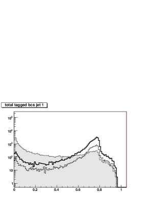
(c)

Figure 2: Distributions of flavour tagging variables for $b\bar{b}$ leading jet in the neutrino channel: (a) b-tag; (b) c-tag; (c) c-tag with b background only. Solid curves are SM background, dashed curves are Higgs background sample and filled histograms are the signal.

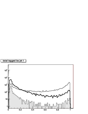
(a)

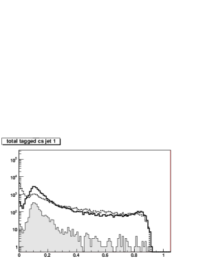
(b)

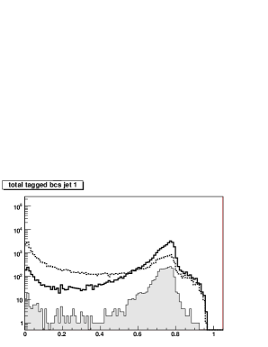
(c)

Figure 3: Distributions of flavour tagging variables for gg leading jet in neutrino channel: (a) b-tag; (b) c-tag; (c) c-tag with b background only. Solid curves are SM background, dashed curves are Higgs background sample and filled histograms are the signal.

The tagging of jets works well. B-jets have relatively long lifetimes and decay topology with up to two secondary vertices and this makes them very distinct. Gluonic jets are tagged as light quark jets.

2.2.2 Hadronic Channel

In the hadronic channel both the Higgs and Z bosons decay into two partons (quarks or gluons) resulting in a 4-jet configuration. For the signal, the invariant mass of two jets is required to be consistent with the Higgs mass and the other two jets should have a mass corresponding to the Z boson. To reduce combinatorial effects, kinematic fitting [4, 13] is performed to identify jets from the Higgs boson and jets from the Z boson. Jet pairing is performed before kinematic fitting. For the 4-jet events we have 6 possible pairings of the jets and 3 possible associations of the 4 jets to the Z and H bosons. For the 6 possible pairings we calculate the invariant mass of each pair and compare with the masses of bosons. For each event we calculate

$$d=(m_{ij}-m_{Z})^{2}+(m_{kl}-m_{H})^{2}$$ (1)

The pairing that minimizes d is chosen. The signal four-jet configuration has, on average, the leading and third jets coming from the Higgs boson and the second and last jets coming from the Z boson.

The kinematic constraints used for the fitter are the jet four-momenta, centre of mass energy (250 GeV) and the invariant mass difference of two jet pairs.

Classification of the hadronic channel requires that no leptons are present in the event and a minimum of 170 GeV of visible energy. Apart from the variables used in the neutrino channel, the other variables/cuts applied in the hadronic channel are the angle between Z boson jets and the invariant mass of jets coming from the Z boson. Table 3 shows the selection cuts in the hadronic channel.

Cuts			selection	value
1.			number of charged tracks per jet	$>$ 4
2.			$-\log(y_{min}$)	$<$ 2.7
3.			thrust	$<0.95$
4.			$\cos(\theta_{thrust})$	$<0.96$
5.	$105^{\circ}$	$<$	angle between jet 1 and 3	$<165^{\circ}$
6.	$70^{\circ}$	$<$	angle between jet 2 and 4	$<160^{\circ}$
7.	110 GeV	$<$	invariant mass of Higgs candidate after fit	$<$ 140 GeV
8.	80 GeV	$<$	invariant mass of Z candidate after fit	$<$ 110 GeV
9.			Highest reconstructed photon energy	$<$ 10 GeV

Table 3: Selections for the four-jet analysis.

Tables 4 and  5 show the number of events before and after pre-selection cuts for $b\bar{b}$ and gg in the neutrino channel.

Cuts	SM background	Higgs background	Signal
(i) Before Classification	9275594683	17816	35629
(0) After Classification	39398366	11875	30985
(1)	18601753	8821	24398
(2)	13921271	7582	20736
(3)	8737017	6472	18391
(4)	7943851	5977	17130
(5)	5871237	5681	16339
(6)	4898312	5678	16326
(7)	1917231	5633	16108
(8)	1561432	5622	16108
(9)	967312	5486	15805

Table 4: Number of $b\bar{b}$ events before channel classification, after channel classification and after pre-selection cuts in the hadronic mode.

Cuts	SM background	Higgs background	Signal
(i) Before Classification	9275594683	50453	2992
(0) After Classification	39398366	39894	2965
(1)	18601753	30717	2503
(2)	13921271	26119	2199
(3)	8737017	22977	1887
(4)	7943851	21396	1738
(5)	5871237	20373	1648
(6)	4898312	20357	1648
(7)	1917231	20103	1638
(8)	1561432	20092	1638
(9)	967312	19860	1611

Table 5: Number of gg events before channel classification, after channel classification and after pre-selection cuts in the hadronic mode.

The main backgrounds at this stage are fully hadronic WW and ZZ pairs, and 2-fermion pairs. As in the neutrino channel, events that survive the pre-selection cuts undergo a neural network analysis to help further discriminate the signal and background. The input variables to the neural network include all pre-selection variables and also the jet flavour tagging outputs produced using the LCFI package. Figures 4,  5,  6 and  7 show distributions of the three LCFI flavour tags, ‘b-tag’, ‘c-tag’ and ‘c-tag with b background only’ for the highest (leading) and second highest energy b- and gluon jets.

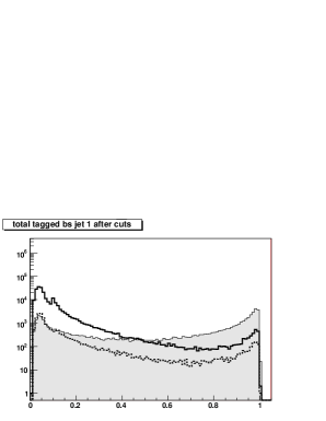
(a)

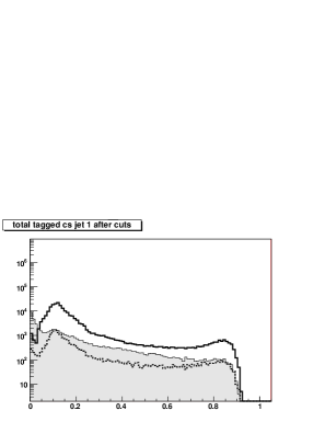
(b)

(c)

Figure 4: Distributions of flavour tagging variables for $b\bar{b}$ in hadronic channel: Leading jet (a) b-tag; (b) c-tag; (c) c-tag with b background only.

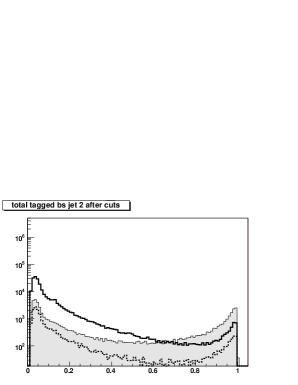
(a)

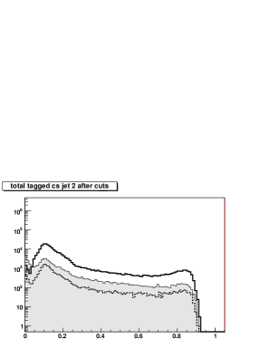
(b)

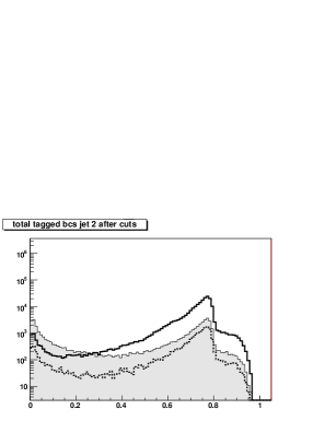
(c)

Figure 5: Distributions of flavour tagging variables for $b\bar{b}$ in hadronic channel: Second jet (a) b-tag; (b) c-tag; (c) c-tag with b background only.

(a)

(b)

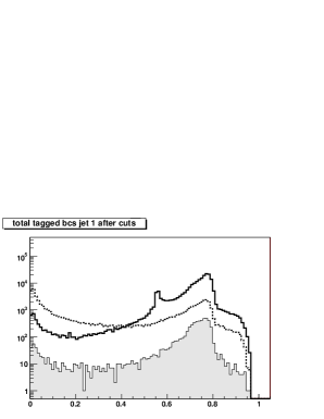
(c)

Figure 6: Distributions of flavour tagging variables for gg in hadronic channel: Leading jet (a) b-tag; (b) c-tag; (c) c-tag with b background only.

(a)

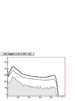
(b)

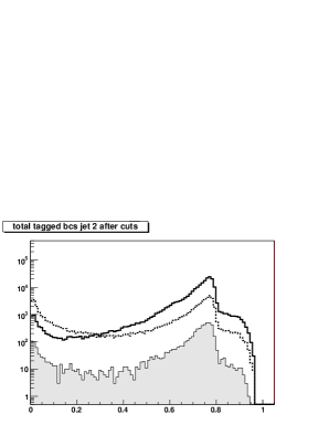
(c)

Figure 7: Distributions of flavour tagging variables for gg in hadronic channel: Second jet (a) b-tag; (b) c-tag; (c) c-tag with b background only.

2.2.3 Di-jet Mass Resolution

Jet energy measurements are a crucial part of Higgs studies and the measurement of the Higgs mass distribution width is important. Figures 8 and  9 show the reconstructed visible mass distribution of Higgs decays to $b\bar{b}$, $c\bar{c}$ and gg in the neutrino and hadronic channels respectively. The histograms are fit with a single gaussian which is not always adequate but nevertheless allows qualitative analysis. In the neutrino channel the $b\bar{b}$ and $c\bar{c}$ systems have broader mass widths than the gluons because of extra neutrinos coming from b- abd c-hadron semi-leptonic decays. The gluon system has a smaller width in the neutrino channel compared to the hadronic channel where the width of the gluon system is broader due to combinatorics. This information was not explicitly used in the analysis. Figure 10 shows the $b\bar{b}$, $c\bar{c}$ and gg Higgs mass distribution in the hadronic channel after kinematic fitting.

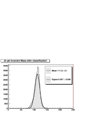
(a)

(b)

(c)

Figure 8: Di-jet invariant mass (GeV) in the neutrino channel: (a) $b\bar{b}$; (b) $c\bar{c}$ and (c) gg.

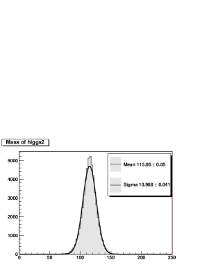
(a)

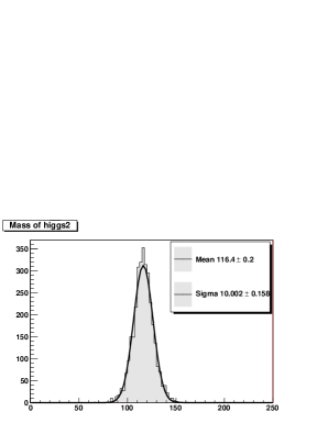
(b)

(c)

Figure 9: Di-jet invariant mass of the Higgs candidate (GeV) in the hadronic channel before kinematic fitting: (a) $b\bar{b}$; (b) $c\bar{c}$ and (c) gg.

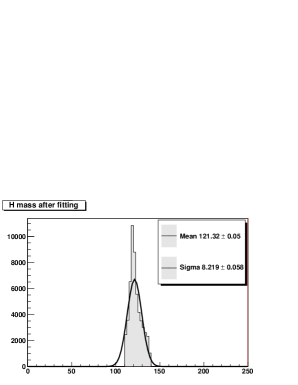
(a)

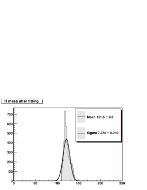
(b)

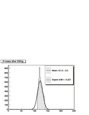
(c)

Figure 10: Hadronic channel after kinematic fitting: (a) b di-jet mass; (b) c di-jet mass; (c) gluon di-jet mass.

2.3 Determination of Branching Ratios

The branching ratio of the Higgs boson decay to quarks and gluons was calculated using events that passed the final neural network selection. The calculation was done by normalising the signal cross section to the inclusive Higgs cross section, $\sigma_{ZH}$ = 209$\pm$9.8 fb, as determined in an independent recoil mass analysis performed for the SiD Letter of Intent [14]. The branching ratio is then given by

$$BR(H\rightarrow f\bar{f})=\frac{\sigma_{Hff}}{\sigma_{ZH}}$$ (2)

where $f$ represents the daughter decay products from the Higgs. The relative accuracy of the the branching ratio takes into account both the relative signal cross section uncertainty and the relative Higgs-strahlung uncertainty given as

$$\frac{\Delta BR}{BR}=\sqrt{\left(\frac{\Delta\sigma_{Hff}}{\sigma_{Hff}}\right)^{2}+\left(\frac{\Delta\sigma_{ZH}}{\sigma_{ZH}}\right)^{2}}$$ (3)

with the relative signal cross section uncertainty calculated by

$$\frac{\Delta\sigma_{Hff}}{\sigma_{Hff}}=\frac{\sqrt{signal+background}}{signal}$$ (4)

and the cross-section is calculated as follows

$$\sigma_{Hff}=\frac{N}{\varepsilon_{Hff}L}$$ (5)

where $N$ is the number of signal events after all selections, $\varepsilon$ is the efficiency of signal selection and $L$ is the total integrated luminosity.

The uncertainty in the efficiency is considered negligible, relying on simulations to determine it with sufficient precision. The systematic effects or contributions of the luminosity uncertainty were not considered in this analysis.

The weighted average of the signal cross section and its uncertainty are calculated using cross section and relative uncertainty values obtained from the neutrino and hadronic channels. The weighted average cross section is given by

$$\sigma_{average}=\frac{x(\delta y)^{2}+y(\delta x)^{2}}{(\delta x)^{2}+(\delta y)^{2}},$$ (6)

where $x$ and $y$ are the cross sections in the neutrino and hadronics channels respectively, and $\delta x$ and $\delta y$ are the cross section uncertainties in the neutrino and hadronic channels respectively assuming that the two channels are statistically independent. The uncertainty of the average cross section is then calculated as

$$\delta z=\frac{\delta x*\delta y}{\sqrt{(\delta x)^{2}+(\delta y)^{2}}},$$ (7)

where $\delta z$ is the uncertainty of the weighted average cross section.

The events remaining after preselection are categorized using two neural networks implemented in FANN [15]. For $b\bar{b}$ the first NN is trained to distinguish the SM background from the inclusive Higgs sample and to produce the NN_SM-Higgs output. In the gg case, the first NN is trained to distinguish the SM background from the signal sample and to produce the NN_Sig-SM output. The second NN is trained to distinguish the signal from the Higgs background sample and to produce the NN_Higgs-signal output. The training is done separately for $b\bar{b}$ and for gg, i.e the training is done twice for the first NN and twice for the second NN. Figures 11 and  12 show one-dimensional histograms of the trained neutral network outputs. Two-dimensional plots of the outputs of the trained NNs are shown in Figures 15,  16,  17 and  18. Again, all the histograms are normalized to luminosity 250 fb^-1.

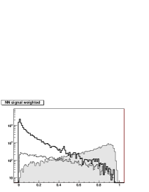
(a)

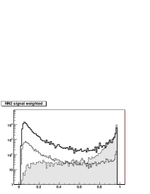
(b)

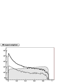
(c)

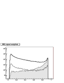
(d)

Figure 11: $b\bar{b}$: Neutrino channel (a) and (b), and Hadronic channel (c) and (d). First NN corresponds to (a) and (c), and Second NN corresponds to (b) and (d). Solid curves are SM background, dashed curves are inclusive Higgs sample (with removed signal) and filled histograms are the signals.

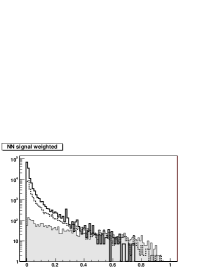
(a)

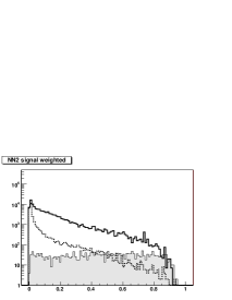
(b)

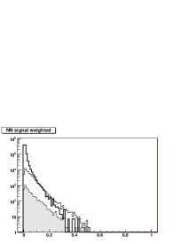
(c)

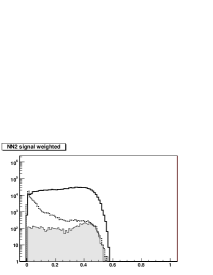
(d)

Figure 12: gg: Neutrino channel (a) and (b), and Hadronic channel (c) and (d). First NN corresponds to (a) and (c), and Second NN corresponds to (b) and (d). Solid curves are SM background, dashed curves are inclusive Higgs sample and filled histograms are the signals.

The final event samples are obtained after applying cuts on First and Second NNs. These cuts are optimized by choosing values of the NNs that maximise the signal-to-noise ratio as shown in Figures 13 and  14.

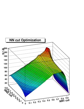
(a)

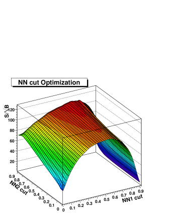
(b)

Figure 13: Neural Network Cut optimization for $b\bar{b}$ : neutrino channel (a) and hadronic channel (b)

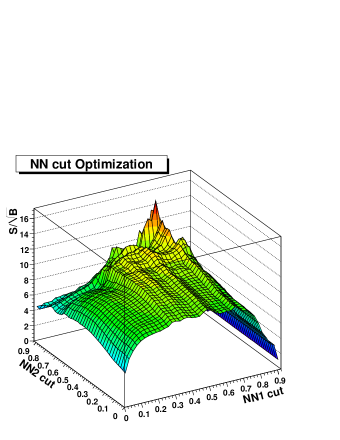
(a)

(b)

Figure 14: Neural Network Cut optimization for gg : neutrino channel (a) and hadronic channel (b)

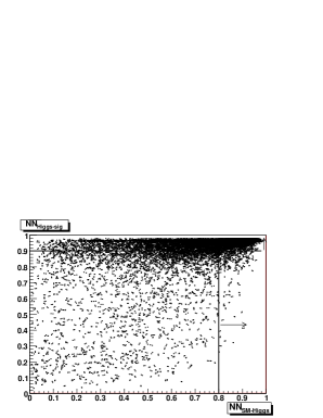
(a)

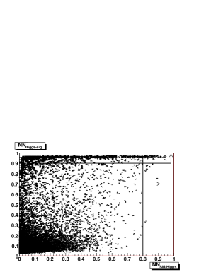
(b)

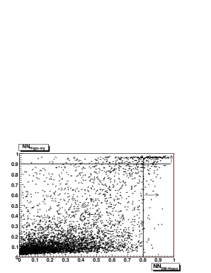
(c)

Figure 15: Neutrino channel $b\bar{b}$: Second NN versus first NN for Signal (a), Standard Model background (b) and Higgs background (c)

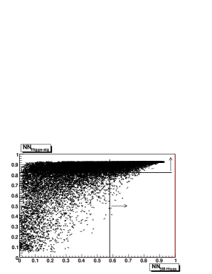
(a)

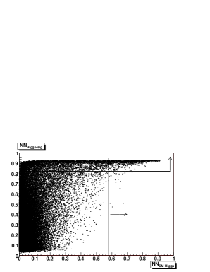
(b)

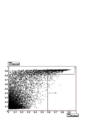
(c)

Figure 16: Hadronic channel $b\bar{b}$: Second NN versus first NN for Signal (a), Standard Model background (b) and Higgs background (c)

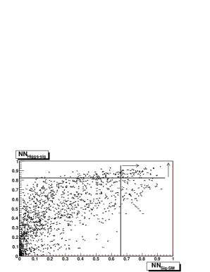
(a)

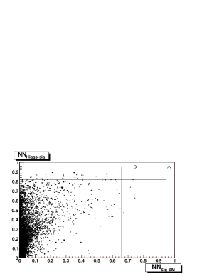
(b)

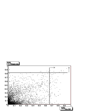
(c)

Figure 17: Neutrino channel gg: Second NN versus first NN for Signal (a), Standard Model background (b) and Higgs background (c)

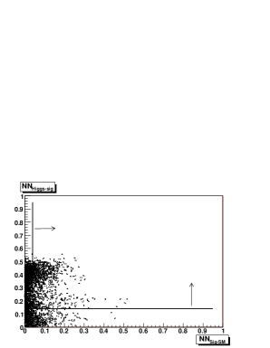
(a)

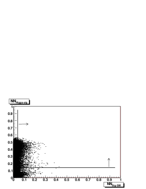
(b)

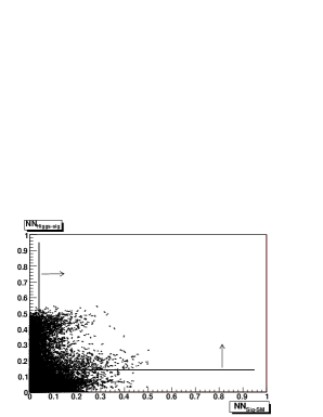
(c)

Figure 18: Hadronic channel gg: Second NN versus first NN for Signal (a), Standard Model background (b) and Higgs background (c)

A summary of the results obtained for both the neutrino and hadronic channels is given in Tables 6 and  7.

	Neutrino	Hadronic	Combined
Signal events	2833	8122
SM background events	220	4700
Higgs background events	55	423
Signal efficiency %	24.465$\pm$0.004	26.213$\pm$0.002
Signal $\sigma_{Hbb}$	142.7$\pm$2.3 fb	142.5$\pm$1.9 fb	142.57$\pm$1.61 fb
Relative uncertainty on $\sigma_{Hbb}$	1.9%	1.4%	1.1%

Table 6: Measurement results of H$\rightarrow b\bar{b}$ branching ratio.

	Neutrino	Hadronic	Combined
Signal events	32	524
SM background events	0	3621
Higgs background events	4	1431
Signal efficiency %	3.245$\pm$0.006	17.673$\pm$0.007
Signal $\sigma_{Hgg}$	15.1$\pm$1.9 fb	15.6$\pm$2.6 fb	15.41$\pm$1.74 fb
Relative uncertainty on $\sigma_{Hgg}$	18.7%	14.2%	11.3%

Table 7: Measurement results of H$\rightarrow$gg branching ratio.

Table 8 shows the summary of the uncertainties of the Higgs branching ratios to $b\bar{b}$ and gg. Also shown in the table is the uncertainty of the Higgs branching ratio to $c\bar{c}$ as given in [4]

Channel	$\frac{\Delta BR}{BR}$ %
H$\rightarrow b\bar{b}$	4.8
H$\rightarrow c\bar{c}$	8.4
H$\rightarrow gg$	12.2

Table 8: Uncertainties of hadronic Higgs decay branching ratios.

3 Conclusion

The measurement of the Higgs boson decay branching ratios to bottom quarks and gluons, for a neutral SM Higgs boson of mass 120 GeV, has been studied at a centre-of-mass of energy of $\sqrt{s}$ = 250 GeV and a total integrated luminosity of 250$\displaystyle\int$fb^-1. The analysis is based on full detector simulation and realistic event reconstruction. The uncertainties on the branching ratios are found to be 4.8% and 12.2% for bb and gg respectively. The uncertainty in the bb branching ratio is dominated by the uncertainty on the inclusive Higgs-strahlung cross section. A good performance of flavour tagging and the use of neural networks in event selection are critical in obtaining these results.

References

- [1] International Linear Collider Reference Design Report, ILC Global Design Effort and Worl Wide Study, August, 2007.
- [2] A. Djouadi, M. Spira and P.M. Zerwas, Phys. Lett. B264 (1991) 440; S. Dawson, Nucl. Phys. B359 (1991) 283; D. Graudenz, M. Spira and P.M. Zerwas, Phys. Rev. Lett. 70 (1993) 1372; M. Spira, A. Djouadi, D. Graudenz and P.M. Zerwas, Nucl. Phys. B453 (1995) 17.
- [3] A. Djouadi, J. Kalinowski and M. Spira, HDECAY: a Program for Higgs Boson Decays in the Standard Model and its Supersymmetric Extensions, Comp.Phys.Comm. 108 (1998), 56.
- [4] Y. Banda, T. Lastovicka, A. Nomerotski, “Measurement of the Higgs boson decay branching ratio to charm quarks at the ILC” arXiv:0909.1052v3 [hep-ph]
- [5] T. Kuhl, K. Desch, “Simulation of the measurement of the hadronic branching ratios for a light Higgs boson at the ILC”, LC-PHSM-2007-001.
- [6] W. Kilian, T. Ohl and J. Reuter, “WHIZARD: Simulating Multi-Particle Processes at LHC and ILC”, arXiv:0708.4233 [hep-ph].
- [7] T. Sjostrand, S. Mrenna and P. Skands, “PYTHIA 6.4 physics and manual”, JHEP 0605, 026 (2006) [arXiv:hep-ph/0603175].
- [8] S. Agostinelli et al, “GEANT4 a simulation toolkit”, Nuclear Instruments and Methods in Physics Research A 506 (2003) 250-303.
- [9] J. Allison et al, “Geant4 developments and applications”, IEEE Transactions on Nuclear Science 53 No. 1 (2006) 270-278.
- [10] http://www.lcsim.org/software/slic/doxygen/html/ .
- [11] Yu.L. Dokshitzer In: Proc. Workshop on Jet Studies at LEP and HERA, Durham, 1990, J. Phys G17(1991), p.1572. S. Catani, Yu.L. Dokshitzer, M. Olsson, G. Turnock and B.R. Webber Phys. Lett B269(1991), p.432
- [12] http://hepwww.rl.ac.uk/LCFI/; LCFI Collaboration, “LCFIVertex package: vertexing, flavour tagging and vertex charge reconstruction for the design of an ILC vertex detector”, Nuclear Inst. and Methods in Physics Research, A 610 (2009), pp. 573-589.
- [13] B. List, J. List, “MarlinKinfit: An Object-Oriented Kinematic Fitting Package”, LC-TOOL-2009-001.
- [14] SiD Collaboration, “Silicon Detector Letter of Intent”, http://silicondetector.org/display/SiD/LOI .
- [15] http://leenissen.dk/fann/ [leenissen.dk]