Aharonov-Bohm effect in many-electron quantum rings

Abstract

The Aharonov-Bohm effect is investigated in two-dimensional, single-terminal quantum rings in magnetic fields by using time-dependent density-functional theory. We find multiple transport loops leading to the oscillation periods of $h/(en)$, where $n$ is the number of loops. We show that the Aharonov-Bohm oscillations are relatively weakly affected by the electron-electron interactions, whereas the ring width has a strong effect on the characteristics of the oscillations. Our results propose that in those experimental semiconductor quantum-ring devices that show clear Aharonov-Bohm oscillations the electron current is dominated by a few states along narrow conduction channels.

I Introduction

The Aharonov-Bohm (AB) effect is one of the most distinct physical phenomena which illustrates the importance of the quantum mechanical phase. AB1 ; AB2 In the AB effect, a charged particle acquires a phase shift

$$\phi=2\pi e/h\int_{\gamma}\mathbf{A}\cdot\mathrm{d}\mathbf{r}$$ (1)

from the vector potential $\mathbf{A}$ while traveling along the path $\gamma$. The existence of this phase shift can be verified, for example, by measuring the current through a quantum ring (QR) in a uniform perpendicular magnetic field. The electrons traveling along right and left arms of the QR gain a relative phase shift

$$\phi_{r}-\phi_{l} =\frac{2\pi e}{h}\left(\int_{\gamma_{r}}\mathbf{A}\cdot\mathrm{d}\mathbf{r}-\int_{\gamma_{l}}\mathbf{A}\cdot\mathrm{d}\mathbf{r}\right)$$

$$=\frac{2\pi e}{h}\int_{S}\mathbf{B}\cdot\mathrm{d}\mathbf{s}=2\pi\Phi/\Phi_{0},$$ (2)

where the surface integral yields the magnetic flux $\Phi$ through the QR, and $\Phi_{0}=h/e$ is the magnetic flux quantum. The resulting current is then a periodic function of $\Phi/\Phi_{0}$.

The AB oscillation was first observed in 1960 by Chambers et al.,Exp0 and the first experiment with the period of $\Phi_{0}$ in a QR configuration was made in 1985 by Webb et al.Exp1 who measured the magnetoresistance of submicron-diameter Au rings. Similar conductance oscillations were later found also in semiconducting QRs.Exp2 ; Exp2b ; Exp3 ; Exp4 ; Exp4b ; Exp8 In addition to being an important concept in quantum mechanics, the AB effect has emerging applications in future computer technologies, random number generation, electron phase microscopy, and holography.Applications

In theory, AB oscillations in QRs have been studied both analytically and numerically. Analytic works Theory1 ; Theory2 ; Theory2b ; Theory3 ; Theory4 have focused on one-dimensional (1D) rings where the electron path itself is not affected by the magnetic field, and thus the situation is different from the experiments.Exp1 ; Exp2 ; Exp2b ; Exp3 ; Exp4 ; Exp4b ; Exp8 Numerical studies include (single-particle) wave-packet simulations in a 1D system, Numerics1 ; Numerics2 and very recently also in a two-dimensional (2D) geometry,Numerics3 as well as 2D tight-binding calculations for conventional QRs Numerics4 and graphene rings. Numerics5 These numerical methods are able to take the effect of Lorentz force into account, in addition to the AB phase shift induced by the vector potential $\mathbf{A}$. The largest effect of the Lorentz force is the asymmetric magnetic-field dependent arm injection of electrons which leads to the decreasing amplitude of the AB oscillations as the magnetic flux through the QR is increased.Numerics1 ; Numerics3 The asymmetric arm injection is qualitatively taken into an account in a recent S-matrix study by Vasilopoulous et al.Theory4 leading to a good agreement with numerical results in Refs. Numerics1, and Numerics3, . In addition to these efforts, the two-particle AB effect has been analyzed in rings where the combined path of independent electrons enclose the magnetic flux. samuelsson

The aim of this paper is to numerically study the transmission effects in a 2D semiconducting QR structure in a static and uniform magnetic field. We use time-dependent density-functional theory which allows us to examine the real-time dynamics, the electron-electron interactions, and the role of the finite ring width (2D character) in the same footing. We find that the width of the conduction channel is a critical parameter for the amplitude of the AB oscillations, whereas the electron-electron interactions have a relatively small effect on the oscillation characteristics. The results give important guidance in assessing the transport dynamics in QR experiments.

The rest of the paper is organized as follows. In Sec. II. we describe the QR structure of interest and the theoretical model of the system. The computational methods used in this work are presented in Sec. III. The results for different number of electrons in the QR are presented, analyzed, and compared qualitatively with experiments in Sec. IV. The work is summarized in Sec. V.

II Model

We consider a model for a semiconductor QR device fabricated in AlGaAs/GaAs structures. Exp2 ; Exp2b ; Exp3 ; Exp4 ; Exp4b ; Exp8 Following the conventional approach in modeling the confined conduction electrons in the material we apply the effective-mass approximation with the GaAs parameters, i.e., the effective mass $m^{\ast}=0.067\,m_{0}$ and the dielectric constant $\varepsilon=12.7\,\varepsilon_{0}$. Hence, the energies, lengths, and times scale as $E_{h}^{\ast}=(m^{\ast}/m_{0})/(\varepsilon/\varepsilon_{0})^{2}E_{h}\approx 11\,\mathrm{meV}$, $a_{0}^{\ast}=(\varepsilon/\varepsilon_{0})/(m^{\ast}/m_{0})a_{0}\approx 10\,\mathrm{nm}$, and $t_{0}^{\ast}=\hbar/E_{h}^{\ast}\approx 60\,\mathrm{fs}$, respectively. In the results we use these effective atomic units unless stated otherwise.

The time-dependent Hamiltonian describing our $N$-electron QR is given by

$$\hat{H} = {\hat{T}}+{\hat{V}}_{ee}+{\hat{V}}_{\rm ext}=\sum_{i=1}^{N}\frac{1}{2m^{\ast}}\left[-i\hbar\nabla_{i}+e\mathbf{A}(\mathbf{r}_{i})\right]^{2}$$ (3)

$$+ \frac{e^{2}}{4\pi\varepsilon}\sum_{i>j}^{N}\frac{1}{|\mathbf{r}_{i}-\mathbf{r}_{j}|}+\sum_{i=1}^{N}v_{ext}(\mathbf{r}_{i},t),$$

where the vector potential is given in the symmetric gauge, $\mathbf{A}=B/2(-y,x,0)$, for the static and uniform magnetic field perpendicular to the QR plane. We neglect the spin effects by considering spin-compensated systems, so that the Zeeman and spin-orbit terms are omitted in the Hamiltonian. We construct a model for a single-terminal QR consisting of $N=1\ldots 10$ electrons and represented by the external potential $v_{ext}(\mathbf{r},t)$. As visualized in Fig. 1,

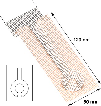
Figure 1: (Color online). External potential describing the quantum ring. The exact form of the potential can be found in Eq. (8). Inset: Schematic image of the quantum ring potential, where the potential for the initial state ($t=0$) is outlined by the dotted line.

the potential consists of the QR confinement and the output terminal. Both the ring and the terminal have a Gaussian-shaped cross section and a tunable width (see Appendix). In addition, we have a linear potential describing a “bias” which is combined to a rectangular potential well at the end of the output terminal. A similar single-terminal geometry for a metallic QR (in 1D) was considered already in Ref. (Theory2b, ).

The static initial state is calculated for a quantum well located in the back part of the QR (see the inset of Fig. 1). Then, the QR and the terminal are suddenly opened up and the electrons are propagated (at $t>0$) from the quantum well into the QR device. The opening is described by the Heaviside step function, which is in fact the only time-dependent part in the external potential (and in the Hamiltonian). Details of the potential can be found in the Appendix.

Using a single-terminal device guarantees that there are no undesired effects of electron back-scattering at the input lead. To minimize the back-scattering at the output of the terminal, the length of the channel is relatively large (approximately three times the diameter of the QR). Moreover, we use a large potential well as a “sink” for electrons beyond the output of the terminal. The side length of the rectangular sink is larger than the length of the terminal.

III Method

To examine the time-dependent many-electron system described by the Hamiltonian in Eq. (3) we apply time-dependent density-functional theory Book-Gross (TDDFT). TDDFT is a practical, yet in principle exact approach to many-body dynamics, and it has received significant popularity in, e.g., calculating electronic excitations. Quantum transport diventrabook can be considered as a recent field for TDDFT and it has been approached by both Green function formalism kurth and finite-system time-propagation appel_thesis ; diventrapaper – the latter being the framework in this study.

TDDFT rests on the Runge-Gross theorem Runge-Gross stating that for a given initial state there is one-to-one correspondence between time-dependent one-body density $n(\mathbf{r},t)$ and the time-dependent one-body potential $v_{ext}(\mathbf{r},t)$. It means that a certain time evolution of the density is generated by at most one time-dependent potential. Thus, it is possible to define an auxiliary Kohn-Sham (KS) system of noninteracting electrons moving in time-dependent effective KS potential, such that the density of the noninteracting system is equal to the density of the real system. The KS potential consists of $v_{ext}(\mathbf{r},t)$ (see above), the Hartree potential corresponding to the classical Coulomb interaction, and the exchange-correlation (xc) potential including all the indirect many-body effects. The xc potential is generally non-local in space and time and needs to be approximated in practice. Here we apply the common adiabatic local-density approximation, so that we locally and instantaneously use the xc potential of the static and uniform 2D electron gas. We point out that the ring width is varied within a range that does not lead to the recently reported failure of the 2D local-density approximation in the quasi-1D limit of QRs. ring_LDA

All TDDFT calculations are done with the octopus code package Octopus published under the GPL license. The code has been built on the real-space grid discretization method which allows realistic modeling of QRs in 2D. The calculations proceed as follows: the initial-state configuration is calculated by solving the KS equations for the initial external potential at $t=0$ and a constant, uniform magnetic field $\mathbf{B}$ perpendicular to the plane. The eigenvalues are solved with the conjugate-gradient algorithm. After the initial calculation the KS orbitals are propagated with the external potential at $t>0$ representing the full device while keeping the magnetic field constant. The propagation of the KS orbitals is done by applying enforced time-reversal symmetry approximation for the time-evolution operator $\hat{U}(t,t_{0})$. After the time-dependent calculation the process is started again with a different magnetic field strength. We point out that the final propagation time is limited by undesired back-scattering effects. Therefore, to obtain a measure for the conductance, we monitor the electronic density up to a specific instant in time as explained below.

IV Results

As a measure for the conductivity in our finite system we consider the relative amount of transferred electrons at time $t$ through the ring,

$$N_{r}(\Phi,t)=1-\frac{N(\Phi,t)}{N},$$ (4)

where $N=1\ldots 10$ is the total (fixed) number of electrons, $\Phi$ is the magnetic flux enclosed by the ring, and $N(\Phi,t)$ is the number of electrons in the QR at time $t$, which is obtained by integrating the electron density over a square which contains the QR.

IV.1 One-electron transport

We begin with a single electron propagated through the QR. As an example of the dynamics of the system, the electron density with magnetic flux $\Phi=3\Phi_{0}$ is visualized at different times in Fig. 2.

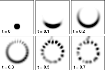
Figure 2: (Color online). One-electron density in a QR with width parameter $a=0.5$ (see Appendix) at different times. Magnetic flux through the QR is $\Phi=3\Phi_{0}$. The symmetry of the density distribution is distorted due to the Lorentz force.

At $t=0$ the density starts to flow through the both arms of the QR. The densities in left and right arms collide near the output at $t\sim 2$ creating a standing wave that oscillates clockwise and counterclockwise in the system, while a part of the density is pumped out from the device. The asymmetric density distribution is caused by the Lorentz force.

The transferred probability density at $t=1$ and $t=2$ is plotted in Figs. 3(a) and (b), respectively.

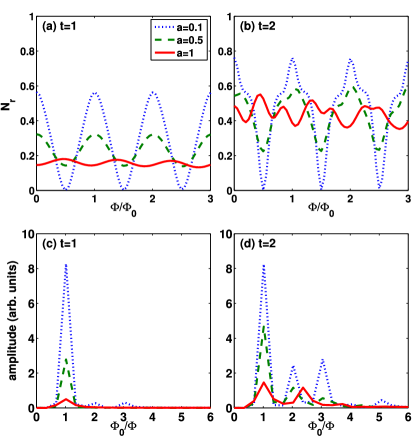
Figure 3: (Color online). Transferred probability density for a single-electron quantum ring at times (a) $t=1$ and (b) $t=2$ as a function of the magnetic flux $\Phi/\Phi_{0}$. (c-d) Corresponding Fourier transforms of the situations in (a) and (b), respectively. Larger $a$ corresponds to a wider ring.

We have considered three different width parameters for the QR channels, $a=0.1$, $0.5$, and $1$ (see Appendix), so that larger $a$ corresponds to larger actual QR width. At $t=1$, a smooth and regular AB oscillation with a period of $\Phi_{0}$ is clearly visible in the conductance. The conduction minima and maxima occur at magnetic flux values corresponding to phase shifts $\pi$ and $2\pi$, respectively [see Eq. (I)]. An exception is the widest ring with $a=1$, where we find a large, almost a half-period phase shift. It is due to transverse density variations and large scattering effects in comparison with thinner rings. In addition, the amplitude of the AB oscillations strongly decreases as a function of $a$. This is due to the fact that the effect of destructive interference becomes smaller when there junction area increases. In other words, the left and right parts of the electron wave packet do not overlap as much as with a thinner output terminal. Increasing further the width of the ring and the output terminal eventually leads to the vanishing of the AB oscillation. Similar destructive effect due to the increasing QR width has been found by Pichugin et al. Numerics4

As shown in Fig. 3(b), at $t=2$ the regular AB oscillation with the period of $\Phi_{0}$ is distorted by oscillations with larger frequencies. The Fourier spectra of $N_{r}$ at $t=1$ and $t=2$ in Figs. 3(c) and (d), respectively, show that at first the major part of the electron transfer occurs at a period of $\Phi_{0}$ in the flux frequency. At larger times the situation changes in an interesting way, namely, we find additional oscillations with AB periods of $\Phi_{0}$, $\Phi_{0}/2$ and $\Phi_{0}/3$. These oscillations arise from multiple transport loops in the ring: a part of the electron density does not flow out from the QR after traveling through one of the arms just once, but it continues to flow in the ring and can travel through an odd number of QR arms before exiting the ring. A similar phenomenon has been recently found in tight-binding Numerics5 and wave-packet calculations for QRs. Numerics3 Multiple transport loops have also been observed experimentally by Chang et al. Exp8

Next we analyze the multiple loops in more detail by considering the initial current split into two QR arms. The right hand part of the current receives a total phase shift

$$\phi_{R,{\rm total}}(n_{r})=\phi_{r}+\left(n_{r}-1\right)\left(\phi_{r}-\phi_{l}\right),$$ (5)

where $n_{r}$ is the number of times the current travels through the right arm, and $\phi_{r}$ ($\phi_{l}$) is the phase shift obtained while traveling through right (left) arm once. Similar equation holds for the left hand part of the current

$$\phi_{L,{\rm total}}(n_{l})=\phi_{l}+\left(n_{l}-1\right)\left(\phi_{l}-\phi_{r}\right).$$ (6)

The total phase difference of the interfering currents can be obtained from Eqs. (I), (5) and (6) as

$$\phi_{R,{\rm total}}-\phi_{L,{\rm total}}=\frac{2\pi\Phi}{\Phi_{0}/\left(n_{r}+n_{l}-1\right)},$$ (7)

which leads to oscillation with periods of $\Phi_{0}/n$, where $n$ is a positive integer. The amplitude of the flux frequency corresponding to the AB period of $\phi_{0}$ does not increase considerably at $t=1...2$: the probability density traveled through only one arm is small at the output of the QR at $t=2$. Proceeding further in time leads to more amplitude peaks for flux frequencies corresponding to periods $\Phi_{0}/n$. According to 2D wave-packet calculations by Chaves et al. Numerics3 this effect is not visible in systems having smooth lead-ring connections.

The effect of the Lorentz force is visible in the densities plotted in Fig. 2. The perpendicular magnetic field favors the other arm of the QR and produces an uneven distribution of the density in the arms. The effect is not that visible in conductance graphs in Fig. 3 since our electrons start from rest. Szafran et al. report increasing maximum of the conductance oscillation together with the decreasing amplitude when the magnetic field is increased: the Lorentz force bends the path of the incoming electrons so that the probability of electron reflection at the input of the device decreases. The effect of the Lorentz force is much smaller in our simulations, since we do not model the scattering effects at the entrance of the QR device.

IV.2 Many-electron transport

Next we consider the electron transport with several electrons. The relative transferred number of electrons for $N=6$ and the corresponding Fourier spectrum are shown in Figs. 4(a) and 4(b).

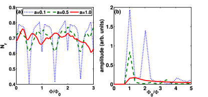
Figure 4: (Color online). (a) Transferred relative number of electrons for a six-electron quantum ring at time $t=3$ as a function of the magnetic flux $\Phi/\Phi_{0}$. (b) Corresponding Fourier transform of the situation in (a). Larger $a$ corresponds to a wider ring.

We find that increasing the number of electrons does not remove the regular AB oscillations, but the system seems to become more sensitive to changes in the width of the ring and the output terminal. The sensitivity appears as strong variations in $N_{r}$ as a function of $a$. They are due to complex electron-electron interaction effects, which, especially in the case of large $a$, have also significant transverse contributions. The thinnest ring with width parameter $a=0.1$ shows signs of oscillations with phase difference of $\pi$ emerging from the interference of scattered and unscattered electron densities. In this case the scattering occurs predominantly along the transport channel.

An explicit view on the effects of electron-electron interactions is given in Fig. 5,

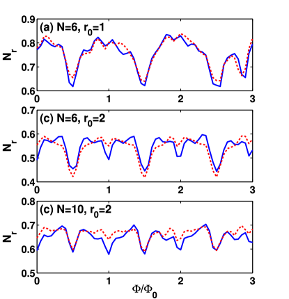
Figure 5: (Color online). Transferred relative number of electrons for different quantum rings with (dashes lines) and without (solid lines) interactions. The width parameter is $a=0.5$ in all cases. (a) $N=6,\ r_{0}=1$. (b) $N=6,\ r_{0}=2$. (c) $N=10,\ r_{0}=2$.

where we compare the noninteracting situation (solid lines) to the interacting one (dashed lines). The conductances are very similar. This is the case even if the radius of the ring is doubled [see Fig. 5(b)], so that the system is relatively more strongly interacting (note that the Coulomb energy scales as $~{}r^{-1}$, whereas the kinetic energy scales as $~{}r^{-2}$). Although the enlargement of the QR notably increases the difference between the two situations, the qualitative picture remains; most importantly, the AB periodicity remains the same. However, the interactions seem to make the local minima at $\Phi=n\Phi_{0}$ less pronounced compared to system without interactions. This corresponds to a smaller amplitude in oscillations with phase shift of $\pi$. Generally, the increase in $N$ leads to the damping of the oscillation amplitudes as shown in the comparison of the six- and ten-electron QRs in Figs. 5(b) and 5(c).

Our results above show that the conductance is sensitive to both the width of the QR as well as the number of electrons confined in the ring. The effects are, however, different in the sense that while increasing the width leads to drastic changes in the AB oscillations even for small $N$, the increase in $N$ mainly damps the oscillation amplitudes. In any case, it can be deduced that in semiconductor QRs containing dozens or hundreds of strongly scattering electrons the AB oscillations are unlikely to be visible. Hence, in view of the several experiments on semiconductor QRs where the AB oscillations are clear, Exp1 ; Exp2 ; Exp2b ; Exp3 we may conclude that in a successful transport measurement the current in the semiconductor QR is induced by only the few highest states along a narrow, almost ballistic path. In metallic QRs (see, e.g., Ref. Exp1, ) the situation might be very different.

To qualitatively assess the relative width of the electron path compared with the QR radius we may consider, for example, the experiment of Fuhrer et al.,Exp3 where the ratio between the width and the radius of the QR device is $\Delta r/r_{0}\sim 0.5$. To obtain similar AB oscillation amplitudes as in the experiment for only a single electron, we need to set $\Delta r/r_{0}\sim 0.3$ (here to estimate $\Delta r$ we have cut the density profile at a few percent of its maximum). This geometry already corresponds to a significantly thinner ring than the experimental one, and the difference becomes even larger if $N$ is increased, since then the width in the calculation should be decreased to maintain the oscillation amplitudes. This qualitative analysis suggests that the actual electron path in the experiment is very narrow compared with the width of the device itself.

V Summary

We have investigated the Aharonov-Bohm effect in a many-electron two-dimensional quantum ring with the time-dependent density functional theory by modeling the discharging of a one-terminal device. We have found multiple transport loops leading to Aharonov-Bohm oscillation periods of $\Phi_{0}/n=h/(en)$, where $n$ is the number of loops. The Aharonov-Bohm oscillations are relatively weakly affected by the electron-electron interactions, whereas the ring width has a strong effect on the characteristics of the oscillations. In general, the oscillations are notably distorted when the conduction channels are made wider. Secondly, the increase in the number of electrons leads to the damping of the oscillation amplitudes. Our results suggest that in experiments on semiconductor quantum rings where the Aharonov-Bohm effect is observed, the actual electron path is narrow compared with the device size, and the transport is dominated by a few electrons close to the Fermi level.

Appendix A Quantum-ring potential

The external potential in the Hamiltonian [Eq. (3)] is given by

$$v_{ext}(\mathbf{r},t)=\theta(t)V_{1}(\mathbf{r})+(1-\theta(t))V_{0}(\mathbf{r}),$$ (8)

where $\theta$ is the Heaviside step function, $V_{0}$ is the ground-state potential ($t=0$) and $V_{1}$ is the potential used in the time propagation ($t>0$). The potentials can be written as

$$V_{0}(\mathbf{r}) =\Bigl{(}-Ve^{-\bigl{(}\frac{\sqrt{x^{2}+y^{2}}-r_{0}}{a}\bigr{)}^{2}}$$

$$\times\theta(x^{2}+y^{2}-(r_{0}+d/2)^{2})$$

$$-\frac{V}{1-e^{-\left(r_{0}/a\right)^{2}}}\Bigl{(}e^{-\bigl{(}\frac{\sqrt{x^{2}+y^{2}}-r_{0}}{a}\bigr{)}^{2}}-e^{-\left(r_{0}/a\right)^{2}}\Bigr{)}$$

$$\times\theta((r_{0}+d/2)^{2}-x^{2}-y^{2})\Bigr{)}$$

$$\times\theta(-x)\theta(y_{c}^{2}-y^{2})$$

and

$$V_{1}(\mathbf{r}) =\min\Bigl{(}-Ve^{(y/a)^{2}}\theta(x),-Ve^{-\bigl{(}\frac{\sqrt{x^{2}+y^{2}}-r_{0}}{a}\bigr{)}^{2}}\Bigr{)}$$

$$\times\theta(L_{\rm pipe}+d/2-x)\theta(x^{2}+y^{2}-(r_{0}+d/2)^{2})$$

$$-\frac{V}{1-e^{-\left(r_{0}/a\right)^{2}}}\Bigl{(}e^{-\bigl{(}\frac{\sqrt{x^{2}+y^{2}}-r_{0}}{a}\bigr{)}^{2}}-e^{-\left(r_{0}/a\right)^{2}}\Bigr{)}$$

$$\times\theta((r_{0}+d/2)^{2}-x^{2}-y^{2})$$

$$+V^{\prime}\bigl{(}-x/L_{\rm pipe}-V/V^{\prime}\theta(x-L_{\rm pipe}-d/2)\bigr{)},$$

where $V$ is the depth of the potential ring, $V^{\prime}$ is the steepness of the linear potential, $r_{0}$ is the radius of the potential minima of the ring, $y_{c}$ is the cutoff length of initial quantum-well potential in the y-direction, $a$ is the width parameter of the ring and the channels, $L_{\rm pipe}$ is the distance between the center of the ring and the edge of the potential well, and $d$ is the grid spacing in the simulation box.

Input parameters used in this work are $V=300$, $V^{\prime}=150$, $L_{\rm pipe}=10$, $r_{0}=1$, $r_{0}=2$, $a=0.1$, $a=0.5$,$a=1.0$ and $d=0.005$. In the propagation we have used time steps of $\Delta t=0.0002\ldots 0.0005$. The length and width of the simulation box are $45$ and $10$, respectively.

- (1) Y. Aharonov and D. Bohm, Phys. Rev. 115, 485 (1959).
- (2) Y. Aharonov and D. Bohm, Phys. Rev. 123, 1511 (1961).
- (3) R. G. Chambers, Phys. Rev. Lett. 5, 3 (1960)
- (4) R. A. Webb, S. Washburn, C. P. Umbach, and R. B. Laibowitz, Phys. Rev. Lett. 54, 2696 (1985).
- (5) G. Timp, A. M. Chang, J. E. Cunningham, T.Y. Chang, P. Mankiewich, R. Behringer, and R. E. Howard, Phys. Rev. Lett. 58 2814 (1987).
- (6) K. Ismail, S. Washburn, and K. Y. Lee, Appl. Phys. Lett. 59, 1998 (1991).
- (7) A. Fuhrer, S. Lüscher, T. Ihn, T. Heinzel, K. Ensslin, W. Wegscheider, and M. Bichler, Nature 413, 822 (2001).
- (8) W. G. van der Wiel, Y. V. Nazarov, S. De Franceschi, T. Fujisawa, J. M. Elzerman, E. W. G. M. Huizeling, S. Tarucha, and L. P. Kouwenhoven, Phys. Rev. B 67, 033307 (2003).
- (9) U. F. Keyser, C. Fühner, S. Borck, R. J. Haug, M. Bichler, G. Abstreiter, and W. Wegscheider, Phys. Rev. Lett. 90, 196601 (2003).
- (10) D.-I. Chang, G. L. Khym, K. Kang, Y. Chung, H.-J. Lee, M. Seo, M. Heiblum, D. Mahalu, and V. Umansky, Nat. Phys. 4, 205 (2008).
- (11) J. M. Alberty, Excerpt from the Proceedings of the COMSOL Multiphysics User’s Conference (Paris 2005).
- (12) M. Büttiker, Y. Imry, and M. Y. Azbel, Phys. Rev. A 30 1982 (1984).
- (13) Y. Gefen, Y. Imry, and M. Y. Azbel, Phys. Rev. Lett. 52, 129 (1984).
- (14) M. Büttiker, Phys. Rev. B 32, 1846 (1985).
- (15) E. R. Hedin, R. M. Cosby, Y. S. Joe, and A. M. Satanin, J. Appl. Phys. 97, 063712 (2005).
- (16) P. Vasilopoulos, O. Kálmán, F. M. Peeters and M. G. Benedict, Phys. Rev. B 75, 035304 (2007).
- (17) B. Szafran and F. M. Peeters, Phys. Rev. B 72, 165301 (2005).
- (18) T. Chwiej and K. Kutorasiński, Phys. Rev. B 81, 165321 (2010).
- (19) A. Chaves, G. A. Farias, F. M. Peeters, and B. Szafran, Phys. Rev. B 80, 125331 (2009).
- (20) K. N. Pichugin and A. F. Sadreev, Phys. Rev. B 56, 9662 (1997).
- (21) J. Wurm, M. Wimmer, H. U. Baranger, and K. Richter, Semicond. Sci. Technol. 25, 034003 (2010).
- (22) P. Samuelsson, E. V. Sukhorukov, and M. Büttiker, Phys. Rev. Lett. 92, 026805 (2004).
- (23) For a review, see Time-Dependent Density Functional Theory, Lecture Notes in Physics, edited by M. A. L. Marques, C. A. Ullrich, F. Nogueira, A. Rubio, K. Burke, and E. K. U. Gross (Springer, Berlin, 2006).
- (24) M. Di Ventra, Electrical Transport in Nanoscale Systems (Cambridge University Press, Cambridge, 2008).
- (25) S. Kurth, G. Stefanucci, C.-O. Almbladh, A. Rubio, and E. K. U. Gross, Phys. Rev. B 72, 035308 (2005).
- (26) H. Appel, Ph.D. thesis, Freie Universität Berlin, 2007.
- (27) See, e.g., N. Sai, N. Bushong, R. Hatcher, and M. Di Ventra, Phys. Rev. B 75, 115410 (2007).
- (28) E. Runge and E.K.U. Gross, Phys. Rev. Lett. 52, 997 (1984).
- (29) E. Räsänen, S. Pittalis, C. R. Proetto, and E. K. U. Gross Phys. Rev. B 79, 121305(R) (2009).
- (30) M. A. L. Marques, A. Castro, G. F. Bertsch, A. Rubio, Comput. Phys. Commun. 151, 60 (2003); A. Castro, H. Appel, M. Oliveira, C. A. Rozzi, X. Andrade, F. Lorenzen, M. A. L. Marques, E. K. U. Gross, and A. Rubio, Phys. Stat. Sol. (b) 243, 2465 (2006).