Born-Oppenheimer approximation for open quantum systems within the quantum trajectory approach

Abstract

Based on the quantum trajectory approach, we extend the Born-Oppenheimer (BO) approximation from closed quantum system to open quantum system, where the open quantum system is described by a master equation in Lindblad form. The BO approximation is defined and the validity condition is derived. We find that the dissipation in fast variables benefits the BO approximation that is different from the dissipation in slow variables. A detailed comparison between this extension and our previous approximation (that is based on the effective Hamiltonian approach, see X. L. Huang and X. X. Yi, Phys. Rev. A 80, 032108 (2009)) is presented. Several new features and advantages are analyzed, which show that the two approximations are complementary to each other. Two examples are taken to illustrate our method.

The adiabatic and Born-Oppenheimer (BO) approximations are among the oldest approaches in quantum mechanics Born1930AP ; Born1985ZPhys . The adiabatic approximation tells us that MacKenzie2007PRA ; Tong2005PRL ; Tong2007PRL ; Zhao2008PRA ; Wu2005PRA ; MarzlinPRL for a time-dependent system governed by Hamiltonian $H(t)$, if the system is prepared in one of the eigenstate $|n(t=0)\rangle$ of $H(t=0)$ at $t=0$, it will keep in that eigenstate $|n(t)\rangle$ of $H(t)$ at arbitrary time $t>0$ provided the Hamiltonian $H(t)$ is changed slowly enough. The Born-Oppenheimer approximation was first given by Born and Oppenheimer in 1927 Born1930AP , which can be formulated as follows CPSun1990 : Treating the slow variables as parameters, we first solve the fast variables with fixed slow variables. Using these solution we obtain an effective Hamiltonian for the slow variables. This effective Hamiltonian contains an effective vector potential induced by fast variables. Based on this Hamiltonian we can obtain a wave function with the slow variables. Thus the total wave function can be factorized into a product of two wave functions corresponding to the fast and slow variables. This method has been widely used in physics and quantum chemistry and becomes a fundamental tool in these fields Shu2009PRA ; Cederbaum2008JCP ; Gong2009PRA ; Yi08 ; Bubin2009JCP ; Muskatel2009PS ; Shim2009PLA ; ABramov2009JPB ; Forre2009PRL ; Ruban2008RPP ; Hua2009PRA ; Tiemann2009PRA ; Leth2009PRL .

Due to the unavoidable coupling of quantum systems to its environments, most quantum systems are open and dissipativeweiss93 . The dynamics of open quantum system can be described by the master equationquantumnoisy ; Breuerbook . It is then natural to ask: How to extend these approximations from closed system to open system? The adiabatic approximation has been extended to open systems in different ways, including the Jordan blocks method in Liouville space Sarandy2005PRL ; Sarandy2005PRA , the effective Hamiltonian approach Huang2008PRA ; Tong2008PLA ; Yi2007JPB and in weak dissipation limit Thunstrom2005PRA . Although the approximation based on the effective Hamiltonian approach is equivalent to the Jordan blocks methodYi2007JPB , the effective Hamiltonian approach has advantages that the extension is straightforward and the effective Hamiltonian is easy to give. The BO approximation has been extended based on effective Hamiltonian approach in Ref.Huang2009PRA . In this paper, we shall extend the BO approximation in a different way, which is based on the quantum trajectory approach. Compared with our previous work, this extension exhibits the following new features and advantages. (1) We do not need to extent the Hilbert space. This will save the CPU (computing) time and memory. (2) All eigenstates of the effective Hamiltonian in the method are physical states. (3) The eigenstates are easy to obtain. (4)It is more accurate to treat the jump terms in the master equation than that in our previous method.

Consider a quantum system with two types of variables, a slow one $\vec{X}$ and a fast one $\vec{Y}$. Then we can divide the total Hamiltonian of the system $H$ into two parts

$$H=H_{s}(\vec{X})+H_{f}(\vec{X},\vec{Y}),$$ (1)

where $H_{s}(\vec{X})$ only contains the slow variables $\vec{X}$. The two types of degrees of freedoms couples together through $H_{f}(\vec{X},\vec{Y})$. We start considering dissipation in the fast variables first. The case of decoherence in the slow variables will be discussed later. Assuming the dissipation is in the Lindblad form, the dynamics for such a system can be described by

$$\frac{\partial}{\partial t}\rho=-\frac{i}{\hbar}[H,\rho]+\mathcal{L}\rho,$$ (2)

where the first term on the right hand side represents an unitary evolution while the second term denotes the dissipation. Here we assume the dissipative term can be arranged into the Lindblad form as

$$\mathcal{L}\rho=\frac{1}{2}\sum_{k}(2L_{k}\rho L^{{\dagger}}_{k}-\rho L^{{\dagger}}_{k}L_{k}-L^{{\dagger}}_{k}L_{k}\rho),$$ (3)

where $L_{k}=L_{k}(\vec{Y})$ is the Lindblad operator relevant to the fast variables $\vec{Y}$. $L_{k}\rho L^{{\dagger}}_{k}$ denotes the jump term. Within the frame of quantum trajectory approach, for an initial state $|\phi(t_{0})\rangle$, one can write the state after an infinitesimal time $dt$ as

$$\rho(t_{0}+dt)=\left(1-\sum_{k}dp_{k}\right)|\phi_{0}\rangle\langle\phi_{0}|+\sum_{k}dp_{k}|\phi_{k}\rangle\langle\phi_{k}|,$$ (4)

where $dp_{k}=\langle\phi(t_{0})|L_{k}^{{\dagger}}L_{k}|\phi(t_{0})\rangle dt$ and the new states are defined by

$$|\phi_{0}\rangle=\frac{(1-iH_{\text{eff}}dt/\hbar)|\phi(t_{0})\rangle}{\sqrt{1-\sum_{k}dp_{k}}},$$

$$|\phi_{k}\rangle=\frac{L_{k}|\phi(t_{0})\rangle}{||L_{k}|\phi(t_{0})\rangle||},$$ (5)

with the non-Hermitian effective Hamiltonian defined by $H_{\text{eff}}=H-\frac{i}{2}\hbar\sum_{k}L_{k}^{{\dagger}}L_{k}$. Under this description, the system will jump into the state $|\phi_{k}\rangle$ with probability $dp_{k}$, and evolve according to non-Hermitian effective Hamiltonian $H_{\text{eff}}$ with probability $1-\sum_{k}dp_{k}$. This unraveling is the so-called Monte Carlo wave function method Dalibard1992PRL ; Carmichaelbook ; Molmer1993JOSAB . The difficulty here is that the non-Hermitian Hamiltonian $H_{\text{eff}}$ contains two types of variables, we will solve this problem by applying the BO approximation in the no-jump trajectory only. For the non-jump evolution $|\phi_{0}\rangle$, the time evolution is given by

$$i\hbar\frac{d}{dt}|\Psi(t)\rangle=H_{\text{eff}}|\Psi(t)\rangle.$$ (6)

Our aim is to solve this equation with the help of BO approximation. To this end, we first rewrite $H_{\text{eff}}$ as $H_{\text{eff}}=H_{s}(\vec{X})+H_{f}^{\prime}(\vec{X},\vec{Y})$ with $H_{f}^{\prime}(\vec{X},\vec{Y})=H_{f}(\vec{X},\vec{Y})-\frac{i}{2}\sum_{k}L_{k}^{{\dagger}}L_{k}$. Obviously, $H_{f}^{\prime}(\vec{X},\vec{Y})$ is not Hermitian that includes all non-Hermitian parts of $H_{\text{eff}}$. Taking the slow variables $\vec{X}$ as parameters, we can solve the eigenstates for $H_{f}^{\prime}(\vec{X},\vec{Y})$. We denote its right eigenstates by $|\psi_{n}^{R}(\vec{X})\rangle$ and the corresponding left eigenstates by $\langle\psi_{n}^{L}(\vec{X})|$ with complex eigenvalues $E_{n}(\vec{X})$. These eigenstates satisfy the relations $\langle\psi_{m}^{L}|\psi_{n}^{R}\rangle=\delta_{mn}$ and $\langle\psi_{n}^{R}|\psi_{n}^{R}\rangle=1$ for fixed $\vec{X}$. We also restrict our discussion to the non-degenerate case. In order to solve Eq.(6), we expand the eigenstate of $H_{\text{eff}}$ in terms of $|\psi_{n}^{R}(\vec{X})\rangle$ as

$$|\Phi\rangle=\sum_{n=1}^{N}c_{n}|\varphi_{n}(\vec{X})\rangle|\psi_{n}^{R}(\vec{X},\vec{Y})\rangle,$$ (7)

where $N$ is the dimension of the fast variables $\vec{Y}$ and $c_{n}\ (n=1,2,3,...,N)$ are the expansion coefficients. Substituting Eq.(7) into the eigenvalue equation $H_{\text{eff}}|\Phi\rangle=E|\Phi\rangle$, after simple calculation, we obtain an equation for the wavefunction of the slow variables

$$\sum_{m}\langle\psi^{L}_{n}|H_{s}(\vec{X})|\psi_{m}^{R}\rangle|\varphi_{m}(\vec{X})\rangle+E_{n}(\vec{X})|\varphi_{n}(\vec{X})\rangle=E|\varphi_{n}(\vec{X})\rangle$$ (8)

Define $H_{n,m}(\vec{X})=\langle\psi_{n}^{L}|H_{s}(\vec{X})|\psi_{m}^{R}\rangle$, we can rewrite Eq.(8) in a matrix form as

$$(\mathcal{H}_{0}+\mathcal{H}_{\mathcal{P}})\varphi=E\varphi,$$ (9)

where $\mathcal{H}_{0},~{}\mathcal{H}_{\mathcal{P}}$ and $\varphi$ are defined by

$$\begin{array}[]{c}\mathcal{H}_{0}=\left[\begin{array}[]{cccc}H_{1}{+}E_{1}(\vec{X})&\ 0&\ \cdots&\ 0\\ 0&\ H_{2}{+}E_{2}(\vec{X})&\ \cdots&\ 0\\ \vdots&\ \vdots&\ \ddots&\ \vdots\\ 0&\ 0&\ \cdots&\ H_{N}{+}E_{N}(\vec{X})\end{array}\right],\end{array}$$

$$\begin{array}[]{c}\mathcal{H}_{\mathcal{P}}=\left[\begin{array}[]{cccc}0&\ {H}_{1,2}&\ \cdots&\ {H}_{1,N}\\ {H}_{2,1}&\ 0&\ \cdots&\ {N}_{2,N}\\ \vdots&\ \vdots&\ \ddots&\ \vdots\\ {H}_{N,1}&\ {H}_{N,2}&\ \cdots&\ 0\\ \end{array}\right],\end{array}\begin{array}[]{c}\varphi=\left[\begin{array}[]{c}|\varphi_{1}\rangle\\ |\varphi_{2}\rangle\\ \vdots\\ |\varphi_{n}\rangle\\ \end{array}\right].\end{array}$$ (12)

Here we have omitted the same subscripts for simplicity. Treating $\mathcal{H}_{\mathcal{P}}$ as perturbation, we can solve Eq.(9) by virtue of the standard time-independent perturbation theory. The solution to the zero-order

$$\begin{array}[]{c}\widetilde{\varphi}_{1,k}^{R[0]}=\left[\begin{array}[]{c}|\varphi_{1,k}^{R[0]}\rangle\\ 0\\ \vdots\\ 0\\ \end{array}\right]\end{array},\begin{array}[]{c}\widetilde{\varphi}_{2,k}^{R[0]}=\left[\begin{array}[]{c}0\\ |\varphi_{2,k}^{R[0]}\rangle\\ \vdots\\ 0\\ \end{array}\right]\end{array},$$ (22)

$$\cdots,\quad\cdots,\qquad\quad\begin{array}[]{c}\widetilde{\varphi}_{N,k}^{R[0]}=\left[\begin{array}[]{c}0\\ 0\\ \vdots\\ |\varphi_{N,k}^{R[0]}\rangle\\ \end{array}\right]\end{array},$$ (28)

can be obtained by the eigenvalue equation

$$\mathcal{H}_{n}|\varphi_{n,k}^{R[0]}\rangle=E_{n,k}^{[0]}|\varphi_{n,k}^{R[0]}\rangle,$$ (29)

where $\mathcal{H}_{n}=(H_{n}(\vec{X})+E_{n}(\vec{X}))$ is the zero-order effective Hamiltonian for the slow variables. From these zeroth-order solutions, one can obtain the higher-order correction accordingly. The condition with which we can neglect the higher-order correction safely is

$$\left|\frac{\langle\varphi_{n^{\prime},k^{\prime}}^{L[0]}|H_{n^{\prime},n}|\varphi_{n,k}^{R[0]}\rangle}{E_{n^{\prime},k^{\prime}}^{[0]}-E_{n,k}^{[0]}}\right|\ll 1,~{}~{}\text{for all}~{}~{}k^{\prime},n^{\prime}\neq k,n,$$ (30)

where $\langle\varphi_{n^{\prime},k^{\prime}}^{L[0]}|$ is the left eigenstate of non-Hermitian Hamiltonian $\mathcal{H}_{n}$.

Next we consider the dissipation about the slow variables. The method used in this case is very similar to the discussion given above. In this case, the Lindblad operator is replaced by $X_{k}$ and it is a function of slow variables only, i.e., $X_{k}=X_{k}(\vec{X})$. In the non-jump trajectory, we divide the non-Hermitian Hamiltonian as $H_{\text{eff}}=H_{s}^{\prime}(\vec{X})+H_{f}(\vec{X},\vec{Y})$, where $H_{s}^{\prime}(\vec{X})=H_{s}(\vec{X})-\frac{i}{2}\sum_{k}X_{k}^{{\dagger}}X_{k}$. The method to find the eigenstates and eigenvalues for $H_{f}$ is the same as for a closed system. These eigenstates are denoted by $|\psi_{n}(\vec{X})\rangle$ with corresponding eigenvalues $E_{n}(\vec{X})$. We can handle the slow variables in the same way. The only difference is $H_{n,m}(\vec{X})$ in Eq.(8) defined as $H_{n,m}(\vec{X})=\langle\psi_{n}|\left(H_{s}(\vec{X})-\frac{i}{2}\sum_{k}X_{k}^{{\dagger}}X_{k}\right)|\psi_{m}\rangle$. The zero-order effective Hamiltonian $\mathcal{H}_{n}$ for slow variables in non-jump trajectory can be similarly obtained. Compared with the closed system, this Hamiltonian includes a non-Hermitian (usually anti-Hermitian) correction $\langle\psi_{n}|-\frac{i}{2}\sum_{k}X_{k}^{{\dagger}}X_{k}|\psi_{n}\rangle$, which comes from the dissipation.

According to the discussion given above, we can solve the dynamics governed by the non-Hermitian Hamiltonian $H_{\text{eff}}$ via expanding the total state as $|\Phi\rangle=\sum_{n,k}c_{n,k}|\varphi_{n,k}^{[0]}\rangle|\psi^{(R)}_{n}\rangle$. Then the Monte Carlo simulation for Eq.(2) is the following. We divide the total evolution time $T$ into several steps. The interval of each step is $dt$. In each step, a random number $\varepsilon$ which distributes in the unit interval $[0,1]$ uniformly is chosen to determine the jump process. If $\varepsilon\leq\sum_{k}dp_{k}$, the total state jumps into the corresponding state according to the corresponding Lindblad operator, i.e., for $\varepsilon\leq dp_{1}$, it jumps to $|\phi_{1}\rangle$, for $dp_{1}<\varepsilon\leq dp_{1}+dp_{2}$, it jumps to $|\phi_{2}\rangle\cdots$. If $\varepsilon>\sum_{k}dp_{k}$, it has no-jump process. The system evolves according to the non-Hermitian Hamiltonian $H_{\text{eff}}$ and the BO approximation is used. This process is repeated as many time as $n_{\text{step}}=T/dt$, and this single evolution gives a quantum trajectory. We can recover the final state of the system by averaging over different quantum trajectories.

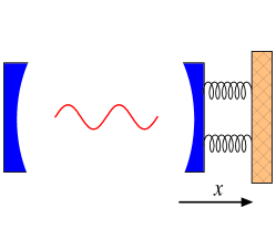
Figure 1: (Color online) Schematic illustration of a Fabry-Pérot cavity with an oscillating mirror at the right end.

In the following, we shall present two examples to illustrate our method. After these two examples, we will give a detailed comparison with our previous work Huang2009PRA . First, we consider a Fabry-Pérot(FP) cavity with an oscillating mirror at one end, acting as a quantum-mechanical harmonic oscillator. Such system can be described by the following Hamiltonian

$$H=\hbar\omega a^{{\dagger}}a-\hbar\chi a^{{\dagger}}ax+\frac{p^{2}}{2m}+\frac{1}{2}m\Omega^{2}x^{2},$$ (31)

where $\omega$ is the frequency of the cavity field with the creation and annihilation operator $a^{{\dagger}}$ and $a$, respectively. $m,\Omega,x$ and $p$ denote the mass, frequency, displacement, and momentum of the oscillating mirror, respectively. $\chi=\omega/L$ is the coupling constant between the cavity field and the mirror. $L$ denotes the length of the cavity. Taking the cavity dissipation into account, the Lindblad operator in this example is $L_{1}=\sqrt{\gamma}a$. The non-Hermitian effective Hamiltonian for the non-jump trajectory can be written as

$$H_{\text{eff}}=\hbar(\omega-\frac{i}{2}\gamma)a^{{\dagger}}a-\hbar ga^{{\dagger}}a(b+b^{{\dagger}})+\hbar\Omega(b^{{\dagger}}b+\frac{1}{2}),$$ (32)

where $b=\sqrt{\frac{m\Omega}{2\hbar}}(x+\frac{ip}{m\Omega})$ and $g=\chi\sqrt{\frac{\hbar}{2m\Omega}}$. Usually, the characteristic frequency of cavity field can reach the order of about $10^{14}$ Hz, which is much higher than the nano-mechanical resonator frequency $10^{9}$ Hz achieved by current experiments Gong2009PRA . Under this condition, we can divide this Hamiltonian into two parts as $H_{\text{eff}}=H_{s}+H_{f}$ with $H_{s}=\hbar\Omega(b^{{\dagger}}b+\frac{1}{2})$ and $H_{f}=\hbar(\omega-\frac{1}{2}i\gamma)a^{{\dagger}}a-\hbar ga^{{\dagger}}a(b+b^{{\dagger}})$. The eigenstate for the fast variables $H_{f}$ is $|\psi_{n_{a}}^{R}\rangle=|n_{a}\rangle$, where $|n_{a}\rangle$ is the Fock state for the mode $a$, and corresponding left eigenstate $\langle\psi_{n_{a}}^{L}|=\langle n_{a}|$ and eigenvalue $E_{n_{a}}=\hbar(\omega-i\gamma)n_{a}-\hbar gn_{a}(b+b^{{\dagger}})$. Putting these into Eq.(29) and following the BO approximation process, we obtain the Hamiltonian for the slow variables as

$$\mathcal{H}_{n_{a}}{=}\hbar\Omega(b^{{\dagger}}b{+}\frac{1}{2}){-}\hbar gn_{a}(b{+}b^{{\dagger}}){+}\hbar(\omega-\frac{1}{2}i\gamma)n_{a}.$$ (33)

This Hamiltonian can be solved by a displacement of the Fock state Gong2009PRA as

$$|\varphi_{n_{a},n_{b}}^{R}\rangle=D(\alpha(n_{a}))|n_{b}\rangle,$$

$$E_{n_{a},n_{b}}=\hbar\Omega(n_{b}+\frac{1}{2})+\hbar(\omega-\frac{1}{2}i\gamma)n_{a}-\frac{\hbar g^{2}}{\Omega}n_{a}^{2},$$

where $D(\alpha)=e^{A^{{\dagger}}\alpha-A\alpha^{*}}$ is the displacement operator with $A=b-\alpha$, and $\alpha(n_{a})=\frac{n_{a}g}{\Omega}$, $|n_{b}\rangle$ is the Fock state for mode $b$. Note that in this model, the off-diagonal elements of the perturbation $\mathcal{H}_{\mathcal{P}}$ is zero, so the BO solution $|\varphi_{n_{a},n_{b}}^{R}\rangle$ for the non-jump trajectory is an exact solution. We study the dynamics for such a Hamiltonian according to the method given above and compare this solution to the solution obtained by the Runge-Kutta method in Fig.2. We choose $|\Phi(0)\rangle=\frac{1}{2}(|0\rangle+|1\rangle)(|0\rangle+|1\rangle)$ as the initial state. To make the effects of dissipation more strikingly, we choose the parameters as $\omega=100\Omega$, $g=0.1\Omega$ in the simulation. In Fig.2(a) we study the entanglement between the vibration of the mirror and the cavity field. We choose negativity Vidal2002PRA as the measure of entanglement for mixed state. In the simulation, the density matrix is calculated by averaging over different runs, i.e., from the state vectors $|\psi_{i}(t)\rangle$ for the different trajectories, the density matrix can be constructed as $\rho(t)=\frac{1}{N}\sum_{i}^{N}|\psi_{i}(t)\rangle\langle\psi_{i}(t)|$. Then we can calculate the negativity for $\rho(t)$. We find that the Hamiltonian Eq.(31) can produce entanglement. The dissipation decreases the entanglement gradually, and the larger the dissipation is, the faster the entanglement decays. In Fig.2(b) we plot the average value of the coordinate $x$ for the oscillating mirror as a function of $\Omega t$. From the figure we find that when the system is a closed system, the average value of the coordinate for the mirror oscillates with time. The dissipation moves the curve left. Similarly, the strength of the dissipation determines the displacement. In our simulation, we average our results over $\mathcal{N}=150$ runs. To check the validity of our method, we compare our results with the results from the Runge-Kutta method. We use the fidelity Fidelity as the measure of difference between two density matrix. For mixed state, the fidelity is defined as $F(\rho_{1},\rho_{2})=\text{Tr}\sqrt{\sqrt{\rho_{1}}\rho_{2}\sqrt{\rho_{1}}}$. This fidelity reaches 1 when the two states are same. In Figs.2(c) and (d) we plot the fidelity between the BO solution and the Runge-Kutta method as a function of $\Omega t$ for different $\gamma$. It is obvious that the fidelities are always larger than $99.9\%$ in our simulation for $\mathcal{N}=150$ trajectories . The error is smaller than $0.1\%$. This confirms that our method can reproduce dissipation dynamics for open system efficiently.

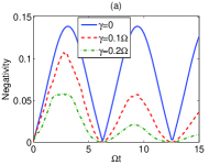
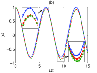
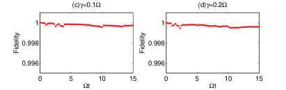
Figure 2: (Color online) (a) The entanglement measured by the negativity as a function of $\Omega t$. (b) The average value of the coordinate $\langle x\rangle$ (in units of $\sqrt{\frac{\hbar}{2m\Omega}}$) as a function of $\Omega t$. (c) and (d) The fidelity between the QTA solution and numerical simulation (Runge-Kutta method). Other parameters in the simulation are $\omega=100\Omega$, $g=0.1\Omega$. The results are obtained by averaging over $\mathcal{N}=150$ runs.

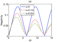
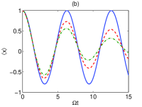
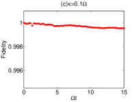
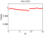
Figure 3: (Color online) The same as Fig. 2 for dissipation in slow variables.

Next we briefly discuss the dissipation in the slow variables for this model. In this case, we also assume the dissipation is in the Lindblad form, then the Lindblad operator reads $X_{1}=\sqrt{\kappa}b$ and the non-Hermitian effective Hamiltonian for the non-jump trajectory is

$$H_{\text{eff}}=\hbar\omega a^{{\dagger}}a-\hbar ga^{{\dagger}}a(b+b^{{\dagger}})+\hbar\Omega(b^{{\dagger}}b+\frac{1}{2})-\frac{1}{2}i\hbar\kappa b^{{\dagger}}b.$$ (34)

Divide it into two parts as $H_{\text{eff}}=H_{s}+H_{f}$ with $H_{s}=\hbar\Omega(b^{{\dagger}}b+\frac{1}{2})-\frac{1}{2}i\hbar\kappa b^{{\dagger}}b$ and $H_{f}=\hbar\omega a^{{\dagger}}a-\hbar ga^{{\dagger}}a(b+b^{{\dagger}})$. The eigenstates for the fast variables are $|\psi\rangle=|n_{a}\rangle$ with eigenvalues $E_{n_{a}}=\hbar\omega n_{a}-\hbar gn_{a}(b+b^{{\dagger}})$. With these knowledge, we obtain the zero-order effective Hamiltonian for the slow variables as

$$\mathcal{H}_{n_{a}}=\hbar\Omega_{0}(b^{{\dagger}}b+\frac{1}{2})-\hbar gn_{a}(b+b^{{\dagger}})+\hbar\omega n_{a}+\frac{1}{2}i\hbar\kappa$$ (35)

with $\hbar\Omega_{0}=\hbar\Omega-\frac{1}{2}i\hbar\kappa$. This Hamiltonian can be solved in a similar way with the displacement $\alpha_{0}=\frac{n_{a}g}{\Omega_{0}}$. The calculations are similar to the process where the dissipation in fast variables is taken into account. The numerical results for this case is shown in Fig. 3. Two differences can be seen from the figure: (1) When the dissipation in slow variables is taken into account, the entanglement never disappears. (2) The amplitude for the average value of the coordinate $\langle x\rangle$ decrease strikingly due to the dissipation. We should note that in this model, the perturbation $\mathcal{H}_{\mathcal{P}}$ is zero in both slow and fast variables’ dissipation case. In general, this condition can not be satisfied (see the second example and Eq.(42)), then we need to restrict the dissipation in slow variables to be weak, because strong dissipation in slow variables enlarge the perturbation $\mathcal{H}_{\mathcal{P}}$, which leads the BO condition to be broken down. This can be understood as follows, large dissipation rate may accelerate the change of slow variables, so that it is hard to distinguish which are the fast variables.

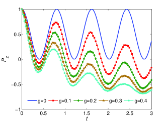
Figure 4: (Color online) The polarization of the neutron along the $z$ axis as a function of time $t$ (in units of $\pi\hbar/\mu B$) for different dimensionless dissipation rate $g$. We have set $\theta=\pi/4$ and initially the spin is in a state $|{+}\frac{1}{2}\rangle$.

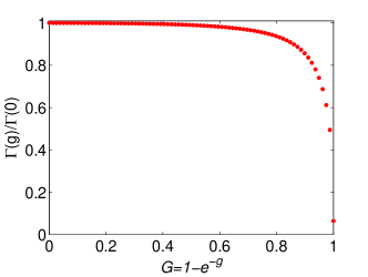
Figure 5: Validity measure $\Gamma(g)$ as a function of the dimensionless dissipation rate $g$. The results have been normalized in units of $\Gamma(g=0)$. Other parameters in the figure are set to satisfy $\hbar/\mu BM^{2}L=10^{-6}$ and $\hbar k_{z}/\mu BML=2\times 10^{-4}$.

In the second example, we consider a neutron moving in a static helical magnetic field,

$$\vec{B}=\vec{B}(z)=B\left(\sin\theta\cos\frac{2\pi z}{L},~{}\sin\theta\sin\frac{2\pi z}{L},~{}\cos\theta\right).$$ (36)

The Hamiltonian for such a system is

$$H=H(z)=\frac{{\vec{p}}^{2}}{2M}+\mu\vec{B}\cdot\vec{\sigma}={H}_{K}+H_{S},$$ (37)

where $\vec{\sigma}=(\sigma^{x},\sigma^{y},\sigma^{z})$ is the Pauli operators. Taking the spin relaxation into account, the Lindblad operator is $L_{2}=\sqrt{\kappa}\sigma^{-}$. Treat the coordinate as parameters, the non-Hermitian Hamiltonian for the non-jump trajectory can be written as

$$H_{\text{eff}} = \mu\vec{B}\cdot\vec{\sigma}-\frac{1}{2}i\hbar\kappa\sigma^{+}\sigma^{-}$$ (40)

$$= \mu B\left(\begin{array}[]{cc}\cos\theta-\frac{1}{2}ig&\sin\theta e^{-{2\pi zi}/{L}}\\ \sin\theta e^{{2\pi zi}/{L}}&-\cos\theta\\ \end{array}\right),$$

where $g=\kappa\hbar/\mu B$ is dimensionless dissipation rate. For each fixed $z$, this non-Hermitian Hamiltonian has two right eigenstates

$$|\psi^{R}_{+}\rangle=\frac{1}{N}\left(\cos\frac{\alpha}{2}|1\rangle+\sin\frac{\alpha}{2}e^{{2\pi zi}/L}|0\rangle\right)$$

$$|\psi^{R}_{-}\rangle=\frac{1}{N}\left(\sin\frac{\alpha}{2}|1\rangle-\cos\frac{\alpha}{2}e^{{2\pi zi}/L}|0\rangle\right),$$

two left eigenstates

$$\langle\psi^{L}_{+}|={N}\left(\cos\frac{\alpha}{2}\langle 1|+\sin\frac{\alpha}{2}e^{{-2\pi zi}/L}\langle 0|\right)$$

$$\langle\psi^{L}_{-}|={N}\left(\sin\frac{\alpha}{2}\langle 1|-\cos\frac{\alpha}{2}e^{{-2\pi zi}/L}\langle 0|\right),$$

and corresponding eigenvalues (in units of $\mu B$)

$$E_{\pm}=-\frac{1}{2}ig\pm\frac{1}{2}\sqrt{16-g^{2}-8ig\cos\theta}$$

In the above expressions, the angle $\alpha$ is defined as

$$\tan\alpha=\frac{4\sin\theta}{4\cos\theta-ig}$$

and the normalized coefficient $N$ is

$$N=\sqrt{\left|\cos\frac{\alpha}{2}\right|^{2}+\left|\sin\frac{\alpha}{2}\right|^{2}}.$$

Note that for a non-zero dimensionless dissipation rate $g$, $\alpha$ is a complex number. In this case, the relation $\sin^{2}\frac{\alpha}{2}+\cos^{2}\frac{\alpha}{2}=1$ holds while $\left|\sin\frac{\alpha}{2}\right|^{2}+\left|\cos\frac{\alpha}{2}\right|^{2}=1$ does not. Put these eigenstates and eigenvalues into Eq.(29), we obtain the zero-order Hamiltonian for the spatial variables as

$$\mathcal{H}_{n}=-\frac{\hbar^{2}}{2M}(\nabla-i\vec{A}_{n})^{2}+E_{n},$$

$$\vec{A}_{n}=i\langle\psi_{n}^{L}|\nabla|\psi_{n}^{R}\rangle,~{}~{}~{}~{}~{}n=+,-.$$ (41)

With these knowledge, we study the population transfer among the internal state for the quantum system. Suppose that we prepare the spin of the neutron in the state $|{+}\frac{1}{2}\rangle$ initially and manipulate the particle moving from $z=0$ to $z=L$ in a fixed time interval $T=3$ (in units of $\pi\hbar/\mu B$). Setting $\theta=\frac{\pi}{4}$, we study the polarization of the neutron along $z$ axis versus time $t$ with different dimensionless dissipation rate $g$, the results are shown in Fig.4. In the simulation we take $\mathcal{N}=400$ trajectories. Some feature can be seen from the figure: When the dissipation is absent, the polarization along $z$ axis oscillates between 0 and 1 as a cosine function of time. The dissipation leads the polarization damping to $-1$ oscillatingly. The stronger the dissipation is, the faster of the damping is. To measure the validity condition, we define a function

$$\Gamma(g)=\max\left\{\left|\frac{\langle\varphi_{n^{\prime},k^{\prime}}^{L[0]}|O_{n^{\prime},n}|\varphi_{n,k}^{R[0]}\rangle}{E_{n^{\prime},k^{\prime}}^{[0]}-E_{n,k}^{[0]}}\right|\right\},$$ (42)

where $O_{n^{\prime},n}=-\frac{\hbar}{2M}(2\langle\psi_{n^{\prime}}^{L}|\nabla|\psi_{n}^{R}\rangle\nabla+\langle\psi_{n^{\prime}}^{L}|\nabla^{2}|\psi_{n}^{R}\rangle),$ to characterize the violation of the BO condition. From Fig.5 we can see that the spin relaxation benefits the approximation. This is same as that in our previous work Huang2009PRA ; Yi2007JPB , and it can also be understood as that the dissipation in fast variables benefit the approximation, because it accelerates the moving of fast variables and the difference between the two types of variables becomes more evident.

It is time to give a detailed comparison between this method and our previous approach Huang2009PRA . We note that the differences come from the two methods itself. This leads to the following distinct features: (1) In Ref. Huang2009PRA , the extension is done by effective Hamiltonian approach, which requires to extend the Hilbert space. In the present paper, the extension is done according to the quantum trajectory approach that does not require to extend the Hilbert space. In addition, in the present paper, if the initial state is pure, the state will always pure in the evolution. (2) In the effective Hamiltonian approach, the extension is simple and straightforward, however, the eigenstates of the Hamiltonian including the fast variables may not be physical states, although it gives a correct dynamics. For example, the last three eigenstates of $H_{S}^{\text{T}}$ in Ref. Huang2009PRA are not physical states. In quantum trajectory approach, the eigenstates are all physical states. (3) The complexity is different. The analytical solution for the non-jump trajectory is easier than the effective Hamiltonian solution. For example, the last three eigenstates for the fast variables $H_{S}^{\text{T}}$ Huang2009PRA is a cubic equation, whose solution is complicated. For a high dimensional open system, the problem become more complicated. But it is relatively easy to solve the eigenstates in this paper, i.e., the non-Hermitian Hamiltonian in non-jump trajectory can be solved more easily than the effective Hamiltonian in Ref. Huang2009PRA . (4) The method in present paper is more accurate to treat the jump term in the master equation. This can be understood as follows. When the dissipation in slow variables is considered, the non-diagonal elements of perturbation $\mathcal{H}_{\mathcal{P}}$ can be divided into two parts as $H_{n,m}=\langle\psi_{n}|H_{s}|\psi_{m}\rangle-\frac{1}{2}i\sum_{k}\langle\psi_{n}|X_{k}^{{\dagger}}X_{k}|\psi_{m}\rangle$. The first part is the same as that in closed system while the second part only contains a term of dissipation. Other part of dissipation is recovered via the jump process. Compared with effective Hamiltonian solution, in which the perturbation includes all parts of dissipation, the quantum trajectory solution is more exact. Before closing this paper, we emphasize that all the discussions in both two methods are restricted to the non-degenerate energy level, i.e., we assume the closed system Hamiltonian is non-degenerate. However, when the dissipation is taken into account, new degeneracy is introduced Tay2007PRA in both methods. For example, in the second example in this paper, even the original system is non-degenerate, the non-Hermitian Hamiltonian $H_{\text{eff}}$ can be degenerate at $\theta=\frac{\pi}{2}$ and $g=4$. In Ref. Huang2009PRA the degenerate occurs at $\theta=\frac{\pi}{2},~{}z=z^{\text{A}}$ and $g=8$. Obviously, the degenerate points in both methods are different, so these two methods are complementary in this sense, in other words, when one method is not available due to the degeneracy, we can choose another method.

In summary, we have extended the BO approximation from closed system to open system by the quantum trajectory approach. An assumption that the dissipation is in Lindblad form is required. The BO approximation is used in the non-jump trajectory and the dynamics can be recovered by the Monte Carlo wave function method. As illustrations, we give two examples to detail our method. The results show that our method can reproduce the dissipation dynamics for such systems efficiently. A detailed comparison with our previous work is also given and discussed.

This work is supported by NSF of China under Grant Nos. 10775023, 10935010 and 10905007.

References

- (1) M. Born and V. Fork, Z. Phys., 74, 439 (1985).
- (2) M. Born and R. Oppenheimer, Annalen der Physik 389, 457 (1927).
- (3) K. P. Marzlin and B. C. Sanders, Phys. Rev. Lett. 93, 160408 (2004); S. Duki, H. Mathur, and O. Narayan, Phys. Rev. Lett. 97, 128901 (2006); J. Ma, Y. P. Zhang, E. G. Wang and Biao Wu, Phys. Rev. Lett. 97, 128902 (2006); K. P. Marzlin and B. C. Sanders, Phys. Rev. Lett. 97, 128903 (2006).
- (4) Z. Y. Wu and H. Yang, Phys. Rev. A 72, 012114 (2005).
- (5) D. M. Tong, K. Singh, L. C. Kwek, and C. H. Oh, Phys. Rev. Lett. 95, 110407 (2005).
- (6) D. M. Tong, K. Singh, L. C. Kwek, and C. H. Oh, Phys. Rev. Lett. 98, 150402 (2007).
- (7) R. MacKenzie, A. Morin-Duchesne, H. Paquette, and J. Pinel, Phys. Rev. A 76, 044102 (2007).
- (8) Y. Zhao, Phys. Rev. A 77, 032109 (2008).
- (9) Chang-Pu Sun and Mo-Lin Ge, Phys. Rev. D 41, 1349 (1990).
- (10) L. S. Cederbaum, J. Chem. Phys. 128, 124101 (2008).
- (11) C. C. Shu, J. Yu, K. J. Yuan, W. H. Hu, J. Yang, and S. L. Cong, Phys. Rev. A 79, 023418 (2009).
- (12) Z. R. Gong, H. Ian, Yu-xi Liu, C. P. Sun, and Franco Nori, Phys. Rev. A 80, 065801 (2009).
- (13) X. X. Yi, H. Y. Sun, and L. C. Wang, arXiv: 0807.2703.
- (14) S. Bubin, J. Komasa, M. Stanke, and L. Adamowicz, J. Chem. Phys. 131, 234112 (2009).
- (15) M. Førre, S. Barmaki, and H. Bachau, Phys. Rev. Lett. 102, 123001 (2009).
- (16) J. B. Shim, M. S. Hussein, M. Hentschel, Phys. Lett. A 373, 3536 (2009).
- (17) B. H. Muskatel, F. Remacle, and R. D. Levine, Phys. Scr. 80 042515 (2009).
- (18) D. I. Abramov, J. Phys. B 41, 175201 (2009); A. V. Matveenko, E. O. Alt, and H. Fukuda, J. Phys. B 42, 165003 (2009).
- (19) A. V. Ruban, and I. A. Abrikosov, Rep. Prog. Phys. 71, 046501 (2009).
- (20) J. J. Hua and B. D. Esry, Phys. Rev. A 80, 013413 (2009).
- (21) E. Tiemann and H. Knöckel, Phys. Rev. A 79, 042716 (2009).
- (22) H. A. Leth, L. B. Madsen, and K. Mølmer, Phys. Rev. Lett. 103, 183601 (2009).
- (23) U. Weiss, Quantum Dissipative Systems(World Scientific, Singapore, 1993).
- (24) H. P. Breuer and F. Petruccione, The Theory of Open Quantum Systems, Oxford University Press, Oxford, 2002.
- (25) C. W. Gardiner, Quantum Noise, Springer, New York, 2000.
- (26) M. S. Sarandy and D. A. Lidar, Phys. Rev. A 71, 012331 (2005).
- (27) M. S. Sarandy and D. A. Lidar, Phys. Rev. Lett. 95, 250503 (2005).
- (28) X. X. Yi, D. M. Tong, L. C. Kwek and C. H. Oh, J. Phys. B 40, 281 (2007).
- (29) D. M. Tong, X. X. Yi, X. J. Fan, L. C. Kwek, C. H. Oh, Phys. Lett. A 372, 2364 (2008).
- (30) X. L. Huang, X. X. Yi, Chunfeng Wu, X. L. Feng, S. X. Yu, and C. H. Oh, Phys. Rev. A 78, 062114 (2008).
- (31) P. Thunström, Johan Åberg, and E. Sjöqvist, Phys. Rev. A 72, 022328 (2005).
- (32) X. L. Huang and X. X. Yi, Phys. Rev. A 80, 032108 (2009).
- (33) J. Dalibard, Y. Castin, and K. Mølmer, Phys. Rev. Lett. 68, 580 (1992).
- (34) K. Mølmer, Y. Castin, and J. Dalibard, J. Opt. Soc. Am. B 10 524 (1993).
- (35) H. Carmichael, An Open Systems Approch to Quantum Optics, (Springer-Verlag, Berlin, 1993).
- (36) G. Vidal and R. F. Werner, Phys. Rev. A 65, 032314 (2002).
- (37) D. Bures, Tran. Am. Math. Soc. 135, 199 (1969); A. Uhlmann, Rep. Math. Phys. 9, 273 (1976).
- (38) B. A. Tay and T. Petrosky, Phys. Rev. A 76, 042102 (2007).