Modeling scaled processes and $1/f^{\beta}$ noise by the nonlinear stochastic differential equations

Abstract

We present and analyze stochastic nonlinear differential equations generating signals with the power-law distributions of the signal intensity, $1/f^{\beta}$ noise, power-law autocorrelations and second order structural (height-height correlation) functions. Analytical expressions for such characteristics are derived and the comparison with numerical calculations is presented. The numerical calculations reveal links between the proposed model and models where signals consist of bursts characterized by the power-law distributions of burst size, burst duration and the inter-burst time, as in a case of avalanches in self-organized critical (SOC) models and the extreme event return times in long-term memory processes. The presented approach may be useful for modeling the long-range scaled processes exhibiting $1/f$ noise and power-law distributions.

Keywords: $1/f$ noise, stochastic processes, point processes, power-law distributions, nonlinear stochastic equations

1 Introduction

The inverse power-law distributions, autocorrelations and spectra of the signals, including $1/f$ noise (also known as $1/f$ fluctuations, flicker noise and pink noise), as well as scaling behavior in general, are ubiquitous in physics and in many other fields, counting natural phenomena, spatial repartition of faults in geology, human activities such as traffic in computer networks and financial markets. This subject is a hot research topic for many decades (see, e.g., [1, 2, 3, 4, 5, 6, 7, 8, 9, 10] and references herein). An up-to-date bibliographic list on $1/f$ noise of more than 1300 papers is composed by Wentian Li [11].

Widespread occurrence of signals exhibiting such a behavior suggests that a generic, at least mathematical explanation of the power-law distributions might exist. Note that the origins of two popular noises, i.e., the white noise – no correlation in time, the power spectrum $S(f)\sim f^{0}$, and integral of the white noise – the Brownian noise (Wiener process), no correlation between increments, the power spectrum $S(f)\sim f^{-2}$, are very well known and understood. $1/f^{\beta}$ noise with $0<\beta<2$, however, cannot be realized and explained in a similar manner and, therefore, no generally recognized explanation of the ubiquity of $1/f$ noise is still proposed.

Despite numerous models and theories proposed since its discovery more than 80 years ago [1], the intrinsic origin of $1/f$ noise still remains an open question. Although in recent years it is annually published about 100 papers with the phrases ‘$1/f$ noise’, ‘$1/f$ fluctuations’ or ‘flicker noise’ in the title, there is no conventional picture of the phenomenon and the mechanisms leading to $1/f$ fluctuations are not often clear. Most of the models and theories have restricted validity because of the assumptions specific to the problem under consideration. Categorization and summary of the contemporary stage of theories and models of $1/f$ noise are rather problematic: on one hand, due to the abundance and variety of the proposed approaches, and on the other hand, for the absence of the recent comprehensive review of the wide-ranging ”problem of $1/f$ noise” and because of the lack of a survey summarizing the current theories and models of $1/f$ noise. We can cite only a pedagogical review of $1/f$ noise subject by Milotti [12]. Wentian Li presents some kind of classification by the categories of publications related with 1/f noise until 2007 [13]. In the peer-reviewed encyclopedia Scholarpedia, [14] there is also a short current review on the subject under the consideration. Thus, we present here only a short and partial categorization of $1/f$ noise models with the restricted list of references.

Until recently, probably the most general and common models, theories and explanations of $1/f$ noise have been based on some formal mathematical description such as fractional Brownian motion, half-integral of the white noise or some algorithms for generation of signals with the scaled properties [15] and popular modeling of $1/f$ noise as the superposition of independent elementary processes with the Lorentzian spectra and proper distribution of relaxation times, e.g., $1/\tau_{relax}$ distribution [16]. The weakness of the later approach is that the simulation of $1/f^{\beta}$ noise with the desirable slope $\beta$ requires finding the special distributions of parameters of the system under consideration, at least a wide range of relaxation time constant should be assumed in order to correlate with the experiments (see also [5, 6, 10, 17]).

Models of $1/f$ noise in some particular systems are usually specific and do not explain the omnipresence of processes with $1/f^{\beta}$ spectrum. Predominantly $1/f$ noise problem has been analyzed in conducting media, semiconductors, metals, electronic devices and other electronic systems [1, 5, 6, 16, 18]. The topic of $1/f$ noise in such systems has been comprehensively reviewed [5], even recently [6]. Nevertheless, despite numerous suggested models, the origin of flicker noise even there still remains an open issue: ”More and more studies suggest that if there is a common regime for the low frequency noise, it must be mathematical rather than the physical one” [6]. Here we can additionaly mention the disputed quantum theory [19] of $1/f$ noise and satisfactorily interpreted $1/f$ noise in quantum chaos [20].

In 1987 Bak, Tang, and Wiesenfeld [21, 22] introduced the notion of self-organized criticality (SOC) with one of the main motivation to explain the universality of $1/f$ noise. SOC systems are nonequilibrium systems driven by their own dynamics to a self-organization. Fluctuations around this state, the so-called avalanches, are characterized by the power-law distributions in time and space, criticality implying long-range correlations. The distributions of avalanche sizes, durations and energies are all seen to be power laws.

Two types of correlations should be distinguished in SOC: the scale-free distribution of their avalanche sizes and temporal correlations between avalanches, bursts or (rare, extreme) events. In the standard SOC models the search of $1/f^{\beta}$ noise is based on the observable power-law dependence of the burst size as a function of the burst duration and the power-law distribution of the burst sizes, with the Poisson distributed interevent times. Such power-laws usually result in the relatively high-frequency power-law, $1/f^{\beta}$, behavior of the power spectrum with the exponent $1.4\lesssim\beta\lesssim 2$ [23, 24]. This mechanism of the power-law spectrum is related to the statistical models of $1/f^{\beta}$ noise representing signals as consisting of different random pulses [25, 26, 27].

It should also be mentioned that originally SOC has been suggested as an explanation of the occurrence of 1/f noise and fractal pattern formation in the dynamical evolution of certain systems. However, recent research has revealed that the connection between these and SOC is rather loose [28]. Though an explanation of $1/f$ noise was one of the main motivations for the initial proposal of SOC, time dependent properties of self-organized critical systems had not been studied much theoretically so far [29].

It is of interest to note, that paper [21] is the most cited paper in the field of $1/f$ noise problem, but it has been shown later on [23, 24] that the proposed in Ref [21] mechanism in SOC systems results in $1/f^{\beta}$ fluctuations with $1.5\lesssim\beta\lesssim 2$ and does not explain the omnipresence of $1/f$ noise. On the other hand, we can point a recent paper [30] where an example of $1/f$ noise in the classical sandpile model has been provided.

It should be emphasized, however, that another mechanism of $1/f^{\beta}$ noise, based on the temporal correlations between avalanches, bursts or (rare, extreme) events, may be the source of the power-law $1/f^{\beta}$ spectra with $\beta\lesssim 1$ [31]. Moreover, SOC is closely related with the observable $1/f^{\beta}$ crackling noise [32], Barkhausen noise [33], fluctuations of the long-term correlated seismic events [34] and $1/f^{\beta}$ fluctuations at non-equilibrium phase transitions [35].

Ten years ago we proposed [8, 9], analyzed [36] and later on generalized [10] a simple point process model of $1/f^{\beta}$ noise and applied it for the financial systems [37]. Moreover, starting from the point process model we derived the stochastic nonlinear differential equations, i.e., the general Langevin equations with a multiplicative noise for the signal intensity exhibiting $1/f^{\beta}$ noise (with $0.5\leq\beta\leq 2$) in any desirable wide range of frequency $f$ [38]. Here we analyze the scaling properties of the signals generated by the particular stochastic differential equations. We obtain and analyze the power-law dependencies of the signal intensity, power spectrum, autocorrelation functions and the second order structural functions. The comparison with the numerical simulations is presented.

Moreover, the numerical analysis reveals the second (reminder, that we start from the point process) structure of the signal composed of peaks, bursts, clusters of the events with the power-law distributed burst sizes $S$, burst durations $T$ and the inter-burst time $\theta$, while the burst sizes are approximately proportional to the squared durations of the bursts, $S\sim T^{2}$. Therefore, the proposed nonlinear stochastic model may simulate SOC and other similar systems where the processes consist of avalanches, bursts or clustering of the extreme events [21, 22, 23, 24, 28, 29, 30, 31, 32, 33, 34, 35, 39].

2 The model

We start from the point process,

$$x(t)=a\sum_{k}\delta(t-t_{k}),$$ (1)

representing the signal, current, flow, etc, $x(t)$, as a sequence of correlated pulses or series of events. Here $\delta(t)$ is the Dirac $\delta$-function and $a$ is a contribution to the signal $x(t)$ of one pulse at the time moment $t_{k}$. Our model is based on the generic multiplicative process for the interevent time $\tau_{k}=t_{k+1}-t_{k}$,

$$\tau_{k+1}=\tau_{k}+\gamma\tau_{k}^{2\mu-1}+\sigma\tau_{k}^{\mu}\varepsilon_{k},$$ (2)

generating the power-law distributed,

$$P_{k}(\tau_{k})\sim\tau_{k}^{\alpha},\quad\alpha=\frac{2\gamma}{\sigma^{2}}-2\mu,$$ (3)

sequence of the interevent times $\tau_{k}$ [10, 37].

Some motivations for equation (2) were given on papers [8, 10, 36, 37]. Additional comments are presented below, after equation (6).

Therefore, in our model the (average) interevent time $\tau_{k}$ fluctuates due to the random perturbations by a sequence of uncorrelated normally distributed random variables $\{\varepsilon_{k}\}$ with zero expectation and unit variance, $\sigma$ is the standard deviation of the white noise and $\gamma\ll 1$ is a coefficient of the nonlinear damping.

Transition from the occurrence number $k$ to the actual time $t$ in equation (2) according to the relation $dt=\tau_{k}dk$ yields the Itô stochastic differential equation for the variable $\tau(t)$ as a function of the actual time,

$$\mathrm{d}\tau=\gamma\tau^{2\mu-2}\mathrm{d}t+\sigma\tau^{\mu-1/2}\mathrm{d}W,$$ (4)

where $W$ is a standard Wiener process. Equation (4) generates the stochastic variable $\tau$, power-law distributed,

$$P_{t}(\tau)=\frac{P_{k}(\tau)}{\left<\tau_{k}\right>}\tau\sim\tau^{\alpha+1},$$ (5)

in the actual time $t$. Here $\left<\tau_{k}\right>$ is the average interevent time. $\tau(t)$ may be interpreted as the average time-dependent interevent time of the modulated Poisson-like process with the distribution of the interevent time

$$P_{p}(\tau_{p})=\frac{1}{\tau\left(t\right)}\mathrm{e}^{-\tau_{p}/\tau\left(t\right)}=n\left(t\right)\mathrm{e}^{-n\left(t\right)\tau_{p}},$$ (6)

where $n(t)=1/\tau(t)$ is the time dependent rate of the process [37].

Additional support for the stochastic model (1) – (6) of the scaled processes and $1/f^{\beta}$ noise is the following. The fluctuations of the intensity of the signals, currents, flows, etc, consisting of the discrete objects (electrons, photons, packets, vehicles, pulses, events, etc) are primarily and basically defined by fluctuations of the (average) interevent, interpulse, interarrival, recurrence, or waiting time. Equation (4) is a special case of the general non-linear Langevin equation

$$\mathrm{d}\tau=d(\tau)\mathrm{d}t+b(\tau)\mathrm{d}W(t)$$ (7)

with the drift coefficient $d(\tau)$ and a multiplicative noise $b(\tau)\xi(t)$ for the (average) interevent time $\tau(t)$, with $\xi(t)$ being a white nose defined from the relation $\mathrm{d}W(t)=\xi(t)\mathrm{d}(t)$. Equation (7) is a straight analogy of the well-known Langevin equation for the continuous random variable $x$. For the process consisting of the discrete objects the intensity of the signal fluctuates due to fluctuations of the rate, i.e., density of the objects in the time axis, which is a consequence of fluctuations of the interarrival or interevent time. Equation (7) in reality represents (in the simplest form) such fluctuations due to random perturbations by white noise.

In papers [8, 9, 10] it has been shown that the small interevent times and clustering of the events make the greatest contribution to $1/f^{\beta}$ noise, low frequency fluctuations and exhibition of the long-range scaled features. Therefore, it is straight to approximate the non-linear diffusion coefficient $b(\tau)$ and the distribution of the interevent time $P_{t}(\tau)$ in some interval of small interevent times $\tau$ by the power-law dependences or expensions,

$$b(\tau)=\sigma\tau^{\mu-\frac{1}{2}},$$ (8)

$$P_{t}(\tau)\sim\tau^{\alpha+1}.$$ (9)

The power-law distribution of the interevent, recurrence, or waiting time is observable in different systems from physics and seismology to the Internet, financial markets and neural spikes (see, e.g., [10, 37, 39]). It should be noted that the multiplicative equations with the drift coefficient $d(\tau)$ proportional to the Stratonovich correction for the drift, leading the transformation from the Stratonovich to the Itô stochastic differential equation [40], i.e., when

$$d(\tau)\sim\frac{1}{2}b(\tau)b^{\prime}(\tau),$$ (10)

with the power-law depending, like (8), diffusion coefficient $b(\tau)$, generates the power-law distribution of the stochastic variable. Equations (2) and (4) are definitely of such kind. Therefore, equation (4) is one of the simplest multiplicative equations for the interevent time, modeling scaled processes, while equation (2) is just the lowest order difference equation following from equation (4) when the step of integration $\Delta t_{k}$ equals the interevent time $\tau_{k}$.

The Itô transformation in equation (4) of the variable from $\tau$ to the averaged over the time interval $\tau$ intensity of the signal $x(t)=a/\tau(t)$ [38] yields the class of Itô stochastic differential equations

$$\mathrm{d}x=\left(\eta-\frac{1}{2}\lambda\right)x^{2\eta-1}\mathrm{d}t_{s}+x^{\eta}\mathrm{d}W$$ (11)

for the signal as function of the scaled time

$$t_{s}=\frac{\sigma^{2}}{a^{3-2\mu}}t.$$ (12)

Here the new parameters

$$\eta=\frac{5}{2}-\mu,\quad\lambda=3+\alpha=\frac{2\gamma}{\sigma^{2}}+2(\eta-1)$$ (13)

have been introduced.

The Fokker-Plank equation associated with equation (11) gives the power-law distribution density of the signal intensity

$$P(x)\sim\frac{1}{x^{\lambda}}$$ (14)

with the exponent $\lambda$.

For $\lambda>1$ distribution (14) diverge as $x\to 0$, and, therefore, the diffusion of $x$ should be restricted at least from the side of small values, or equation (11) should be modified. Thus, further we will consider the modified equation for $x>0$ only,

$$\mathrm{d}x=\left(\eta-\frac{1}{2}\lambda\right)(x_{m}+x)^{2\eta-1}\mathrm{d}t_{s}+(x_{m}+x)^{\eta}\mathrm{d}W,$$ (15)

with the additional small parameter $x_{m}$ restricting the divergence of the power-law distribution of $x$ at $x=0$.

Equation (15) for small $x\ll x_{m}$ represents the linear additive stochastic process generating the Brownian motion with the steady drift, while for $x\gg x_{m}$ it reduces to the multiplicative equation (11).

3 Analysis of the model

The Fokker-Plank equation associated with equation (15) gives the steady-state solution for distribution of $x$,

$$P(x)=\frac{(\lambda-1)x_{m}^{\lambda-1}}{(x_{m}+x)^{\lambda}},\quad x>0,\quad\lambda>1.$$ (16)

We can obtain the power spectral density of the signal generated by equation (15) from equation (28) derived in paper [10]. After some algebra we can write

$$S(f)=\frac{A}{f^{\beta}},\quad f\gg f_{1}=\frac{2+\lambda-2\eta}{2\pi}x_{m}^{2(\eta-1)}$$ (17)

with

$$A=\frac{(\lambda-1)\Gamma(\beta-1/2)x_{m}^{\lambda-1}}{2\sqrt{\pi}(\eta-1)\sin(\pi\beta/2)}\left(\frac{2+\lambda-2\eta}{2\pi}\right)^{\beta-1}$$ (18)

and

$$\beta=1+\frac{\lambda-3}{2(\eta-1)}$$ (19)

for $0.5<\beta<2$, $4-\eta<\lambda<1+2\eta$ and $\eta>1$. Note that the frequency $f$ in equation (17) is the scaled frequency matching the scaled time $t_{s}$ (12).

The autocorrelation function $C(s)$ of the process can be expressed according to Wiener-Khinchin theorem as the inverse Fourier transform of the power spectrum,

$$C(s)=\left<x(t)x(t+s)\right>=\int_{0}^{\infty}S(f)\cos(2\pi fs)\mathrm{d}f.$$ (20)

A pure $1/f^{\beta}$ power spectrum is physically impossible because of the total power would be infinity. Depending on whether $\beta$ is greater or less than one it is necessary to introduce a low frequency cutoff $f_{\min}$ or a high frequency cutoff $f_{\max}$ [41, 42]. For calculation of the autocorrelation function according to equation (20) when $\beta>0$ it is not necessary to introduce the hight frequency cutoff.

Usually one introduces a discontinuous transition to the flat spectrum at the lower cutoff $f_{\min}$ [41, 42]. Here at low frequencies we will insert the smooth transition to the flat spectrum in the vicinity of $f_{0}\sim f_{\min}$, i.e., we will approximate the power spectrum (17) as

$$S(f)=\frac{A}{(f_{0}^{2}+f^{2})^{\beta/2}}=\cases{A/f_{0}^{\beta},\qquad f\ll f_{0},\\ A/f^{\beta},\qquad f\gg f_{0}.}$$ (21)

Inserting (21) into equation (20) we obtain

$$C(s)=\frac{A\sqrt{\pi}}{\Gamma(\beta/2)f_{0}^{\beta-1}}\left(\frac{z}{2}\right)^{h}K_{h}(z),$$ (22)

where $K_{h}(z)$ is the modified Bessel function, $z=2\pi f_{0}s$ and $h=(\beta-1)/2$.

The first two terms of expansion of equation (22) in powers of $z$ are

$$C(s)=\frac{A\sqrt{\pi}}{2\Gamma(\beta/2)f_{0}^{\beta-1}}\left[\Gamma\left(\frac{\beta-1}{2}\right)+\Gamma\left(\frac{1-\beta}{2}\right)(\pi f_{0}s)^{\beta-1}\right]$$ (23)

for $h\neq 0$, i.e, $\beta\neq 1$, and

$$C(s)=AK_{0}(2\pi f_{0}s)\simeq A[-\gamma-\ln(\pi f_{0}s)]=\mathrm{const}-A\ln s$$ (24)

for $h=0$, i.e., for the pure $1/f$ noise with $\beta=1$. Here $\gamma\simeq 0.577216$ is Euler’s constant.

The leading terms of expression (23) are different, depending on whether $\beta<1$ or $\beta>1$. Thus for $h<0$, i.e., when $0<\beta<1$

$$C(s)=\frac{A\Gamma(1-\beta)}{(2\pi s)^{1-\beta}}\sin\left(\frac{\pi\beta}{2}\right)\sim\frac{1}{s^{1-\beta}},$$ (25)

while for $h>0$, i.e., for $1<\beta<3$

$$C(s)=C(0)-Bs^{\beta-1}.$$ (26)

Here

$$C(0)=\left<x^{2}\right>=\int_{0}^{\infty}S(f)\mathrm{d}f=\frac{A\sqrt{\pi}\Gamma\left(\frac{\beta-1}{2}\right)}{2f_{0}^{\beta-1}\Gamma\left(\frac{\beta}{2}\right)}$$ (27)

and

$$B=\frac{A\pi^{\beta+\frac{1}{2}}}{2\Gamma\left(\frac{\beta}{2}\right)\Gamma\left(\frac{\beta+1}{2}\right)\sin\left(\pi\frac{\beta-1}{2}\right)}=-A(2\pi)^{\beta-1}\Gamma(1-\beta)\sin\left(\frac{\pi\beta}{2}\right).$$ (28)

For $\beta=2$ equations (22) and (26) – (28) yield

$$C(s)=C(0)e^{-2\pi f_{0}s}=\frac{A\pi}{2f_{0}}e^{-2\pi f_{0}s}=C(0)-A\pi^{2}s\pm...$$ (29)

It should be noted, that particular cases (24) – (29) of the general expressions (22) and (23) are in agreement with the results of papers [41, 42, 43] obtained with the non-uniform cutoff of the spectrum at low frequency. On the other hand, the introduced parameter $h$ for $\beta\geq 1$ coincides with the Hurst exponent $H$ [42],

$$H=\cases{0,\qquad 0<\beta\leq 1,\\ \frac{1}{2}(\beta-1),\qquad 1<\beta<3,\\ 1,\qquad 3\leq\beta<4.}$$ (30)

The exponent $H$ is associated with the scaling of the second order structural function, or height-height correlation function [41, 42, 43, 44]

$$F(s)=F_{2}^{2}(s)=\left<\left|x(t+s)-x(t)\right|^{2}\right>\sim s^{2H}.$$ (31)

The exponent $H$ characterizes the power-law diffusion rate, as well. This variance of the differenced time series (delayed signal) may be expressed as

$$F(s)=\left<x^{2}(t+s)\right>+\left<x^{2}(t)\right>-2\left<x(t+s)x(t)\right>=2[C(0)-C(s)].$$ (32)

Substituting expressions (20) and (27) into (32) we have

$$F(s)=F_{2}^{2}(s)=4\int_{0}^{\infty}S(f)\sin^{2}(\pi sf)\mathrm{d}f.$$ (33)

For the convergence of integral in (33) at $\beta\leq 1$ we need to cut off the power-law spectrum (17) at high frequency $f_{\max}$. Then the leading terms of the height-height correlation function (33) are

$$F(s)=2A\times\cases{\frac{f_{\max}^{1-\beta}}{1-\beta}\left[1-\frac{\Gamma(2-\beta)}{(2\pi f_{\max}s)^{1-\beta}}\sin\left(\frac{\pi\beta}{2}\right)\right],\qquad 0<\beta<1,\\[0.0pt] ,\qquad\beta=1.}$$ (34)

For $1<\beta<3$ the integral in (33) may be integrated exactly and we have

$$F(s)=-2A\Gamma(1-\beta)\sin\left(\frac{\pi\beta}{2}\right)(2\pi s)^{\beta-1}=2Bs^{\beta-1},\quad 1<\beta<3.$$ (35)

The spatial power spectrum and the height-height correlation function (31) are used for analysis of rough self-affine surfaces and assessing the growth mechanism of thin films [45, 46, 47, 48, 49], as well. There sometimes the violation of the scaling relation $\beta=2H+1$ is observable [46, 47, 50].

Figure 1: Examples of the numerically computed signals according to equations (37) and (38) with the parameters $\eta=2$, $x_{m}=10^{-2}$ and different values of $\beta$ and $\lambda$: $\beta=1/2$ when $\lambda=2$, $\beta=1$ when $\lambda=3$ and $\beta=3/2$ when $\lambda=4$ and the interburst time $\theta_{j}$ as a function of the occurrence number $j$ of the events peaking above the threshold value $x_{th}=0.1$ for the pure $1/f$ noise with $\beta=1$ when $\lambda=3$.

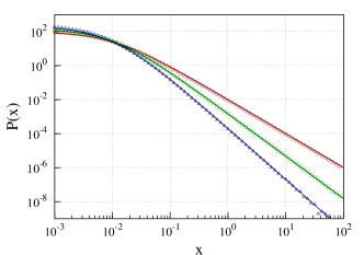
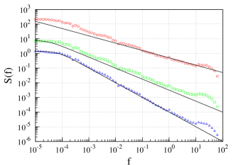
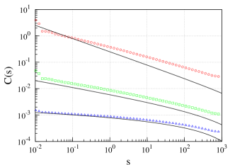
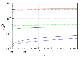
Figure 2: Distribution density, $P\left(x\right)$, power spectral density, $S\left(f\right)$, autocorrelation function, $C(s)$, and the second order structural function, $F_{2}\left(s\right)$, for solutions of equation (15) with $\eta=2$, $x_{m}=10^{-2}$ and different values of the parameter $\lambda$: $\lambda=2$ (circles), $\lambda=2.5$ (squares) and $\lambda=3$ (triangles) in comparison with the analytical results (solid lines) according to equations (16), (18) – (22), (34) and (35), respectively.

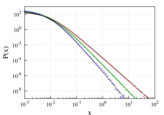
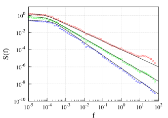
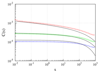
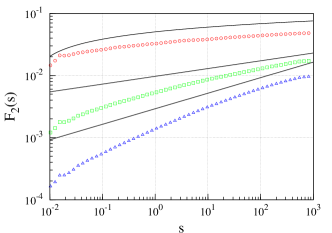
Figure 3: As in figure 2 but for the parameters $\lambda=3$ (circles), $\lambda=3.5$ (squares) and $\lambda=4$ (triangles).

4 Numerical analysis

For the numerical analysis we have to solve equation (15) and analyze the obtained numerical solutions. We can solve equation (15) using the method of discretization with the variable step of integration

$$h_{i}=\Delta t_{i}=\frac{\kappa^{2}}{\left(x_{m}+x_{i}\right)^{l}},$$ (36)

where $\kappa$ is a small parameter while the exponent $l$ rules the dependence of the integration step on the value of the variable $x$. Thus, $l=0$ corresponds to the fixed step, for $l=1$ we have analogy with equation (2) when the step is proportional to the interevent time $\tau_{k}$, $l=2\left(\eta-1\right)$ matches the case when the change of the variable $x$ in one step is proportional to the value of the variable at time of the step [38] and so on. As a result we have the system of the difference equations

$$x_{i+1}=x_{i}+\kappa^{2}\left(\eta-\frac{1}{2}\lambda\right)\left(x_{m}+x_{i}\right)^{2\eta-1-l}+\kappa\left(x_{m}+x_{i}\right)^{\eta-l/2}\varepsilon_{i},$$ (37)

$$t_{i+1}=t_{i}+\frac{\kappa^{2}}{\left(x_{m}+x_{i}\right)^{l}},\quad x_{i}>0.$$ (38)

Here $\varepsilon_{i}$ is a set of uncorrelated normally distributed random variables with zero expectation and unit variance. In the Milstein approximation equation (37) should be replaced by the equation

$$x_{i+1}=x_{i}+\frac{\kappa^{2}}{2}\left(\eta-\lambda\right)\left(x_{m}+x_{i}\right)^{2\eta-1-l}+\kappa\left({}_{m}+x_{i}\right)^{\eta-l/2}\varepsilon_{i}+\frac{\kappa^{2}\eta}{2}\left(x_{m}+x_{i}\right)^{2\eta-1-l}\varepsilon_{i}^{2}.$$ (39)

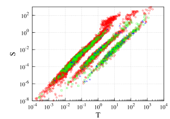
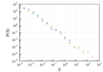
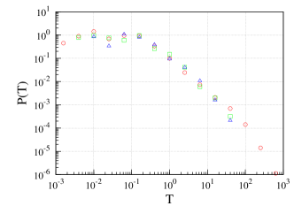
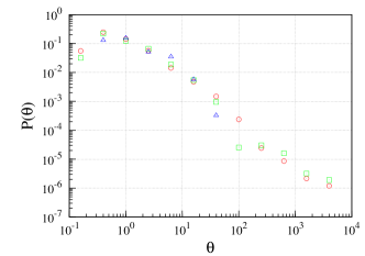
Figure 4: Dependence of the burst size $S$ as a function of the burst duration $T$: traces from the top of the figure for size $S$ above the threshold value $x_{th}=0.02$, 0.1 and 0.5, respectively, distributions of the burst size, $P(S)$, burst duration, $P(T)$, and interburst time, $P(\theta)$, for the peaks above the the threshold value $x_{th}=0.1$. Calculations are as in figures 2 and 3 with the parameters $\eta=2$, $x_{m}=10^{-2}$ and different values of the parameter $\lambda$: $\lambda=2$ (circles), $\lambda=3$ (squares) and $\lambda=4$ (triangles).

Numerical analysis indicate that the variable of equation (15) exhibits some peaks, bursts or extreme events, corresponding to the large deviations of the variable from the appropriate average value. As examples, in figure 1 we show the illustrations of the signals generated according to equation (15) for different slopes of the signal distributions and the dependence of the interburst time $\theta_{j}$ on the burst occurrence number $j$. We see that the the computed signal is composed of bursts of different size with a wide range distribution of the inerburst time. In figures 2 and 3 the numerical calculations of the distribution density, $P\left(x\right)$, power spectral density, $S\left(f\right)$, autocorrelation function, $C(s)$, and the second order structural function, $F_{2}\left(s\right)=\sqrt{F\left(s\right)}$, for solutions of equation (15) with $\eta=2$, $x_{m}=10^{-2}$ and different values of the parameter $\lambda$ are presented. We see rather good agreement between the numerical calculations and the analytical results except for the structural function $F_{2}\left(s\right)$ when $\lambda>3$. Numerical evaluation of the structural function in a case of the steep power-law distribution is problematic, because in the calculation one needs to average (squared) small difference of the rare large fluctuations.

In figure 4 we demonstrate numerically that the size of the generated bursts $S$ is approximately proportional to the squared burst duration $T$, i.e., $S\propto T^{2}$, and asymptotically approximately power-law distributions of the burst size, $P(S)\sim S^{-1.3}$, burst duration, $P(T)\sim T^{-1.5}$ and interburst time, $P(\theta)\sim\theta^{-1.5}$, for the peaks above the threshold value $x_{th}$ of the variable $x(t)$.

It should be noted that the parameter $\eta=2$ yields in equation (4) the additive noise and the linear relaxation of the signal $x=a/\tau$, i.e., the simple (pure) Brownian motion in the actual time of the interevent time with the linear relaxation of the signal.

5 Conclusions

Starting from the multiplicative point process we obtain the stochastic nonlinear differential equations, which generate signals with the power-law statistics, including $1/f^{\beta}$ fluctuations. We derive analytical expressions for the probability density of the signal, for the power spectral density, the autocorrelation function, the second oder structural function and demonstrate that the analytical results are in agreement with the results of numerical simulations. The numerical analysis of the equations reveals the secondary structure of the signal composed of peaks or bursts, corresponding to the large deviations of the variable $x$ from the proper average fluctuations. The burst sizes are approximately proportional to the squared duration of the burst. According to the theory [24, 27] such dependence for the uncorrelated bursts should result in $1/f^{\beta}$ noise with $\beta\approx 2$ in the relatively high-frequency region. The power-law distribution $P(\theta)$ of the interburst time $\theta$ indicates in correlation of the burst occurrence times and may result in $1/f^{\beta}$ noise with $\beta<2$, similarly to the point process model [8, 9, 10]. On the other hand, the proposed model reproduces $1/f$ noise models and the processes not only in SOC and crackling systems but it is related with the clustering Poisson process [51], $1/f$ noise due to diffusion of defects or impurity centers in semiconductors [52], $1/f$ noise in nanochannels, single-channel and ion channel currents [53], etc. Therefore, the presented and analyzed model may be used for simulation the long-range scaled processes exhibiting $1/f$ noise, power-law distributions and self-organization.

References

References

-
[1]
Johnson J B, 1925 Phys. Rev. 26 71
Schottky W, 1926 Phys. Rev. 28 74 -
[2]
Mandelbrot B B, 1963 J. Business 36 394
Allan D W, 1966 Proc. IEEE 54 221
Granger C W J, 1966 Econometrica 34 150 -
[3]
Beran J, 1994 Statistics for Long-Memory Processes (New York: Chapman and Hall)
Mandelbrot B B, 1997 Fractals and Scaling in Finance (New York: Springer)
Mandelbrot B B, 1999 Multifractals and 1/f Noise: Wild Self-Affinity in Physics (New York: Springer)
Mantegna R N and Stanley H E, 2000 An Introduction to Econophysics: Correlations and Complexity in Finance (Cambridge, UK: Cambridge University Press)
Racher S T (ed), 2003 Handbook of Heavy Tailed Distributions in Finance (Amsterdam: Elsevier B V) -
[4]
Voss R F and Clarke J, 1975 Nature 258 317
Press V H, 1978 Comments. Astrophys. 7 103
Gardner M, 1978 Sci. Am. 238(4) 16
Newman M E J, 2005 Contemp. Phys. 46 323 -
[5]
Hooge F N, Kleinpenning T G M and Vadamme L K J, 1981 Rep. Prog. Phys. 44 479
Dutta P and Horn P M, 1981 Rev. Mod. Phys. 53 497
Kogan S M, 1985 Usp. Fiz. Nauk 145 285 [1985 Sov. Phys. Usp. 28 170]
Weissman M B, 1988 Rev. Mod. Phys.60 537
Van Vliet C M, 1991 Solid-State Electron. 34 1
Zhigalskii G P, 1997 Usp. Fiz. Nauk 167 623 [1997 Sov. Phys. Usp. 40 599]
Zhigal’skii G P, 2003 Usp. Fiz. Nauk 56 449 - [6] Wong H, 2003 Microelectron. Reliab. 43 585
-
[7]
Musha T and Higuchi H, 1976 Jap. J. Appl. Phys. 15 1271
Lawrence A, Watson M G Pounds K A and Elvis M, 1987 Nature 325 695
Gilden D L, Thornton T and Mallon M W, 1995 Science 267 1837
Gabaix X, Gopikrishnan P, Plerou V and Stanley E, 2003 Nature 423 267
Carbone A, Kaniadakis G and Scarfone A M, 2007 Eur. Phys. J. B 57 121
Smeets R M M, Keyser U F, Dekker N H and Dekker C, 2008 PNAS 105 417 - [8] Kaulakys B and Meškauskas T, 1998 Phys. Rev. E 58 7013
- [9] Kaulakys B, 1999 Phys. Lett. A 257 37
- [10] Kaulakys B, Gontis V and Alaburda M, 2005 Phys. Rev. E 71 051105
- [11] Li W, 2009 http://www.nslij-genetics.org/wli/1fnoise
- [12] Milotti E, 2002 Preprint physics/0204033
- [13] Li W, 2007 http://www.nslij-genetics.org/wli/1fnoise/index-by-category.html
- [14] Scholarpedia, 2009 http://www.scholarpedia.org/article/1/f_noise
-
[15]
Mandelbrot B B, Van Ness J W, 1968 SIAM Rev. 10 422
Masry E, 1991 IEEE Trans. Inform. Theory 37 1173
Milotti E, 1995 Phys. Rev. E 51 3087
Mamontov Y V and Willander M, 1997 Nonlinear Dynamics 12 399
Ninness B, 1998 IEEE Trans. Inform. Theory 44 32
Jumarie G, 2005 Appl. Math. Lett. 18 739
Milotti E, 2005 Phys. Rev. E 72 056701
Ostry D I, 2006 IEEE Trans. Inform. Theory 52 1609
Erland S and Greenwood P E, 2007 Phys. Rev. E 76 031114 -
[16]
Bernamont J, 1937 Ann. Phys. (Leipzig) 7 71
Surdin M, 1939 J. Phys. Radium 10 188
Van der Ziel A, 1950 Physica (Amsterdam) 16 359
McWhorter A L, 1957 In: Semiconductor Surface Physics, ed R H Kingston (Philadelphia: Univ. of Pennsylvania) p 207
Ralls K S, Skocpol W J, Jackel L D, Howard R E, Fetter L A, Epworth R W and Tennant D M, 1984 Phys. Rev. Lett. 52 228
Rogers C T and Buhrman R A, 1984 Phys. Rev. Lett. 53 1272
Palenskis V, 1990 Litov. Fiz. Sb. 30 107 [Lithuanian Phys. J. 30 (2) 1]
Watanabe S, 2005 J. Korean Phys. Soc. 46 646 - [17] Kaulakys B, Alaburda M and Ruseckas J, 2007 AIP Conf. Proc. 922 439
-
[18]
Palenskis V and Shoblitskas Z, 1982 Solid State Commun. 43 761
Kogan S M and Nagaev K E, 1984 Solid State Commun. 49 387
Shtengel K and Yu C C, 2003 Phys. Rev. B 67 165106
Burin A L, Shklowskii B I, Kozub V I, Galperin Y M and Vinokur V, 2006 Phys. Rev. B 74 075205
Muller J, von Molnar S, Ohno Y and Ohno H, 2006 Phys. Rev. Lett. 96 186601
Koch R H, DiVincento D P and Clarke J, 2007 Phys. Rev. Lett. 98 267003
de Sousa R, 2007 Phys. Rev. B 76 245306
Burin A L, Shklowskii B I, Kozub V I, Galperin Y M and Vinokur V, 2008 phys. stat. sol. (c) 5 800
D’Souza A I, Stapelbroek M G, Robinson E W, Yoneyama C, Mills H A, Kinch M A, Skokan M R and Shih H D, 2008 J. Electron. Materials 37 1318 -
[19]
Handel P H, 1975 Phys. Rev. Lett. 34 1492; 34 1495
Kazakov K A, 2008 Physica B 403 2255
Foster S, 2008 Phys. Rev. A 78 013820 -
[20]
Relano A, Gomez J M G, Molina R A, Retamosa J, and Faleiro E, 2002 Phys. Rev. Lett. 98 244102
Salasnich L,2005 Phys. Rev. E 71 047202
Abul-Magd A Y, Dietz B, Friedrich T, and Richter A, 2008 Phys. Rev. E 77 046202 - [21] Bak P, Tang C and Wiesenfeld K, 1987 Phys. Rev. Lett. 59 381
- [22] Bak P, Tang C and Wiesenfeld K, 1988 Phys. Rev. A 38 364
-
[23]
Jensen H J, Christensen K and Fogedby H C, 1989 Phys. Rev. B 40 7425
Takayasu H, 1989 Phys. Rev. Lett. 63 2563
Kertesz J and Kiss L B, 1990 J. Phys. A 23 L433
Jaeger H M and Nagel S R, 1992 Science 255 1523
Paczuski M, Maslov S and Bak P, 1996 Phys. Rev. E 53 414
Davidsen J and Schuster H G, 2000 Phys. Rev. E 62 6111
Laurson L, Alava M J and Zapperi S, 2005 J. Stat. Mech. L11001
Laurson L and Alava M J, 2006 Phys. Rev. E 74 066106
Poil S S, van Ooyen A and Linkenkaer-Hansen K, 2008 Human Brain Mapping 29 770 - [24] Kuntz M C and Sethna J P, 2000 Phys. Rev. E 62 11 699
- [25] Heiden C, 1969 Phys. Rev. 188 319
- [26] Schick K L and Verveen A A, 1974 Nature 251 599
-
[27]
Ruseckas J, Kaulakys B and Alaburda M, 2003 Lithuanian J. Phys. 43 p.223; arXiv:0812.4674
Kaulakys B, Alaburda M, Gontis V, Meškauskas T and Ruseckas J, 2007 In: Traffic and Granular Flow’05, eds A Schadschneider, T Poschel, R Kuhne, M Schreckenberg and D E Wolf (Berlin: Springer-Verlag) p 603; arXiv:physics/0512068 - [28] Frigg R, 2003 Stud. Hist. Phil. Sci. 34 613
- [29] Dhar D, 2006 Physica A 369 29
- [30] Baiesi M and Maes C, 2006 EPL 75 413
-
[31]
Davidsen J and Paczuski M, 2002 Phys. Rev. E 66 050101 (R)
Bunde A, Eichner J F, Havlin S and Kantelhardt J W, 2004 Physica A 342 308
Bunde A, Eichner J F, Kantelhardt J W and Havlin S, 2005 Phys. Rev. Lett. 94 048701
Eichner J F, Kantelhardt J W, Bunde A and Havlin S, 2007 Phys. Rev. E 75 011128
Blender R, Fraedrich K, Sienz F, 2008 Nonlin. Processes Geophys. 15 557 -
[32]
Sethna J P, Dahmen K A and Myers C R, 2001 Nature 410 242
Eggenhoffner R, Celasco E and Celasco M, 2007 FNL 7 L351 -
[33]
Cote P J and Meisel L V, 1991 Phys. Rev. Lett. 67 1334
Meisel L V and Cote P J, 1992 Phys. Rev. B 46 10822
Colaiori F, 2008 Adv. Phys. 57 287 -
[34]
Telesca L, Cuomo V, Lapenna V and Macchiato M, 2002 FNL 2 L357
Davidsen J, Grassberger P and Paczuski M, 2008 Phys. Rev. E 77 066104 -
[35]
Novak U and Usadel K D, 1991 Phys. Rev. B 43 851
Koverda V P, Skokov V N and Skripov V P, 1998 J. Exp. Theor. Phys. 86 953
Fukuda K, Takayasu H and Takayasu M, 2000 Physica A 287 289
Koverda V P and Skokov V N, 2005 Physica A 346 203 -
[36]
Kaulakys B and Meškauskas T, 1999 Nonlinear Anal.: Model. Control 4 87
Kaulakys B and Meškauskas T, 2000 Microelecron. Reliab. 40 1781
Kaulakys B, 2000 Microelecron. Reliab. 40 1787
Kaulakys B, 2000 Lithuanian J. Phys. 40 281 -
[37]
Gontis V and Kaulakys B, 2004 Physica A 343 505; 344 128
Gontis V and Kaulakys B, 2006 J. Stat. Mech. P10016
Gontis V and Kaulakys B, 2007 Physica A. 382 114
Gontis V, Kaulakys B and Ruseckas J, 2008 Physica A. 387 3891 -
[38]
Kaulakys B and Ruseckas J, 2004 Phys. Rev. A 70 020101(R)
Kaulakys B, Ruseckas J, Gontis V and Alaburda M, 2006 Physica A 365 217 -
[39]
Thurner S, Lowen S B, Feurstein M C, Heneghan C, Feichtinger H G and Teich M C, 1997 Fractals 5 565
Schwalger T and Schimansky-Geier L, 2008 Phys. Rev. E 77 031914
Perello J, Masoliver J, Kasprzak A and Kutner R, 2008 Phys. Rev. E 78 036108 -
[40]
Arnold P, 2000 Phys. Rev. E 61 6091
Kupferman R, Pavliotis G A and Stuart A M, 2004 Phys. Rev. E 70 036120 - [41] Theiler J, 1991 Phys. Lett. A 155 480
- [42] Talocia S G, 1995 Phys. Lett. A 200 264
- [43] Caprari R S, 1998 J. Phys. A 31 3205
- [44] Kaulakys B, Alaburda M, Gontis V and Meškauskas T, 2006 In: Conplexus Mundi: Emergent Patterns in Nature, ed M M Novak (Singapore: World Scientific) p 277
- [45] Barabasi A L and Stanley H E, 1995 Fractal Concepts in Surface Growth (Cambridge UK: Cambridge University Press)
- [46] Yang H -N and Lu T -M, 1995 Phys. Rev. B 51 2479
- [47] Zhao Y -P, Cheng C -F, Wang G -C and Lu T -M, 1998 Surface Science 409 L703
- [48] Yanguas-Gil A, Cotrino J, Walkiewicz-Pietrzykowska A and Gonzalez-Elipe A R, 2007 Phys. Rev. B 76 075314
- [49] Palasantzas G, 2008 J. Appl. Phys. 104 053524
- [50] Timashev S F and Polyakov Y S, 2007 FNL 7 R15
-
[51]
Gruneis F, 1984 Physica A 123 149
Gruneis F and Musha T, 1986 Jap. J. Appl. Phys. 25 1504
Gruneis F, 2001 FNL 1 R119
Takayasu H and Takayasu M, 2003 Physica A 324 101
Gontis V, Kaulakys B and Ruseckas J, 2005 AIP Conf. Proc. 776 144 -
[52]
Gruneis F, 2000 Physica A 282 108; Corrigendum 290 512
Gruneis F, 2007 FNL 7 C1 -
[53]
Derksen H E and Verveen A A, 1966 Science 151 1388
Bezrukov S M and Winterhalter M, 2000 Phys. Rev. Lett. 85 202
Siwy Z and Fulinski A, 2002 Phys. Rev. Lett. 89 158101
Banerjee J, Verma M K, Manna S and Ghosh S, 2006 EPL 73 457
Kosinska I D and Fulinski A, 2008 EPL 81 50006