Abstract

We calculate in closed analytical form the one-photon loop radiative corrections to muon Compton scattering $\mu^{-}\gamma\to\mu^{-}\gamma$. Ultraviolet and infrared divergencies are both treated in dimensional regularization. Infrared finiteness of the (virtual) radiative corrections is achieved (in the standard way) by including soft photon radiation below an energy cut-off $\lambda$. We find that the anomalous magnetic moment $\alpha/2\pi$ provides only a very small portion of the full radiative corrections. Furthermore, we extend our calculation of radiative corrections to the muon-nucleus bremsstrahlung process (or virtual muon Compton scattering $\mu^{-}\gamma_{0}^{*}\to\mu^{-}\gamma$). These results are particularly relevant for analyzing the COMPASS experiment at CERN in which muon-nucleus bremsstrahlung serves to calibrate the Primakoff scattering of high-energy pions off a heavy nucleus with the aim of measuring the pion electric and magnetic polarizabilities. We find agreement with an earlier calculation of these radiative corrections based on a different method.

PACS: 12.20.-m, 12.20.Ds, 14.70.Bh

1 Introduction and summary

At present there is much interest in a precise experimental determination of the (charged) pion electric and magnetic polarizabilities, $\alpha_{\pi}$ and $\beta_{\pi}$. Within the systematic framework of chiral perturbation theory the firm prediction, $\alpha_{\pi}-\beta_{\pi}=(5.7\pm 1.0)\cdot 10^{-4}\,$fm³ [1], has been obtained for the (dominant) polarizability difference at two-loop order. However, this chiral prediction is in conflict with the existing experimental determinations of $\alpha_{\pi}-\beta_{\pi}=(15.6\pm 7.8)\cdot 10^{-4}\,$fm³ from Serpukhov [2] and $\alpha_{\pi}-\beta_{\pi}=(11.6\pm 3.4)\cdot 10^{-4}\,$fm³ from Mainz [3], which amount to values more than twice as large. Certainly, these existing experimental determinations of $\alpha_{\pi}-\beta_{\pi}$ raise doubts about their correctness since they violate the chiral low-energy theorem notably by a factor 2.

In that contradictory situation it is promising that the ongoing COMPASS [4] experiment at CERN aims at measuring the pion polarizabilities with high statistics using the Primakoff effect. The scattering of high-energy negative pions in the Coulomb field of a heavy nucleus (of charge $Z$) gives access to cross sections for $\pi^{-}\gamma$ reactions through the equivalent photons method [5]. In practice, one analyzes the spectrum of bremsstrahlung photons produced in the reaction $\pi^{-}Z\to\pi^{-}Z\gamma$ in the so-called Coulomb peak. This kinematical regime is characterized by very small momentum transfers to the nuclear target such that virtual pion Compton scattering $\pi^{-}\gamma^{*}_{0}\to\pi^{-}\gamma$ occurs as the dominant subprocess (in the one-photon exchange approximation). The deviations of the measured spectra (at low $\pi^{-}\gamma$ center-of-mass energies) from those of a point-like pion are then attributed to the pion structure as represented by its electric and magnetic polarizabilities [2] (taking often $\alpha_{\pi}+\beta_{\pi}=0$ as a constraint). It should be stressed here that the systematic treatment of virtual pion Compton scattering $\pi^{-}\gamma^{*}_{0}\to\pi^{-}\gamma$ in chiral perturbation theory yields at the same order as the polarizability difference $\alpha_{\pi}-\beta_{\pi}$ a further pion-structure effect in form of a unique pion-loop correction [6, 7] (interpretable as photon scattering off the “pion-cloud around the pion”). In the case of real pion Compton scattering $\pi^{-}\gamma\to\pi^{-}\gamma$ this loop correction compensates partly the effects from the pion polarizability difference [8]. A minimal requirement for improving future analyses of pion-nucleus bremsstrahlung $\pi^{-}Z\to\pi^{-}Z\gamma$ is therefore to include the loop correction predicted by chiral perturbation theory. At the required level of accuracy it is also necessary to include higher order electromagnetic corrections to the pion-nucleus bremsstrahlung process $\pi^{-}Z\to\pi^{-}Z\gamma$. These radiative corrections of order $\alpha$ have been calculated recently in ref.[9], where explicit analytical expressions for the corresponding one-photon loop amplitudes have been written down. Their implementation into the analysis of the COMPASS data is currently planned.

The setup of the COMPASS experiment [4] gives the possibility to switch (within a short time) from a pion beam to a muon beam which allows for precise acceptance studies with a point-like (purely electromagnetically interacting) particle. In this way the muon-nucleus bremsstrahlung process $\mu^{-}Z\to\mu^{-}Z\gamma$ serves the purpose to calibrate the Primakoff scattering events of high-energy pions off a heavy nucleus (of charge $Z$). Clearly, in order to preserve the level of accuracy one should take into account also the radiative corrections to the Bethe-Heitler cross section, which describes the muon-nucleus bremsstrahlung process $\mu^{-}Z\to\mu^{-}Z\gamma$ only at lowest order. The purpose of the present work is therefore to (re-)calculate the one-photon loop radiative corrections to muon-nucleus bremsstrahlung (or virtual muon Compton scattering). Radiative corrections to bremsstrahlung have been computed already 50 years ago by Fomin in refs.[10, 11]. The analytical expression given in eq.(36) of ref.[11] (in terms of auxiliary functions defined by multiple integrals and derivatives thereof) is somewhat cumbersome for a numerical evaluation. Also, the limiting cases discussed explicitly in refs.[10, 11] do not apply to the kinematics of the COMPASS experiment, in which the muon beam and photon energy are very large, whereas the momentum transfer to the nucleus is very small. In this situation it is helpful to have an independent derivation of these radiative corrections based on a different calculational method as employed in ref.[11]. We are using here the dimensional regularization of ultraviolet and infrared divergent loop diagrams. In particular, we specify as a function of the five independent kinematical variables, the pertinent expressions for the interference terms between one-photon loop and tree diagrams summed over the muon spin and photon polarization states. In this detailed and explicit form our analytical results for the radiative corrections to virtual muon Compton scattering can be readily utilized for analyzing the muon Primakoff data of the COMPASS experiment.

The present paper is organized as follows. Section 2 is devoted to the (simpler) calculation of the one-photon loop radiative corrections to real muon Compton scattering $\mu^{-}\gamma\to\mu^{-}\gamma$. The analogous case of electron Compton scattering has been considered long ago by Brown and Feynman in ref.[12] and the final result for the radiative corrections has been documented in the textbook on quantum electrodynamics by Akhiezer and Berestetskii [13]. As a new element we use here dimensional regularization to treat both ultraviolet and infrared divergencies and we write down in closed analytical form the expressions for the pertinent interference terms between one-photon loop and tree diagrams summed over the muon spin and photon polarization states. While the ultraviolet divergencies drop out in the renormalizable spinor electrodynamics at work, the infrared divergencies get removed (in the standard way) by including soft photon radiation below an energy cut-off $\lambda$. We confirm the absolute correctness of the final formula for these radiative corrections written in eq.(52.12) of the book by Akhiezer and Berestetskii [13]. In the closer analysis, we find that the muon anomalous magnetic moment $\kappa=\alpha/2\pi$ provides only a very small part of the (virtual) radiative corrections. Moreover, we compare these radiative corrections with those to (spin-0) pion Compton scattering and observe strong similarities concerning the energy and angular dependences. In section 3, we extend our calculation of radiative corrections to virtual muon Compton scattering $\mu^{-}\gamma^{*}_{0}\to\mu^{-}\gamma$, where $\gamma^{*}_{0}$ denotes the virtual (Coulomb) photon that couples to the charge of a heavy nucleus in the bremsstrahlung process $\mu^{-}Z\to\mu^{-}Z\gamma$. We derive again analytical expressions for the pertinent interference terms between one-photon loop and tree diagrams summed over the muon spin and photon polarization states. Since these expressions depend now on five independent kinematical variables, they become rather lengthy for some terms. The radiative correction factor arising from the soft photon radiation off the muon (which cancels the infrared divergencies due to the photon-loops) is evaluated together with all its finite pieces in the laboratory frame. For this (soft photon) part the agreement with Fomin’s earlier calculation [11] is obvious. For the (virtual) radiative corrections arising from photon loops the agreement between our and Fomin’s calculation [11] can be verified numerically with good precision.

The presentation of numerical results for the radiative corrections to the muon bremsstrah- lung process $\mu^{-}Z\to\mu^{-}Z\gamma$ in the COMPASS experiment is not pursued here, since that requires specification and implementation of the actual experimental conditions (such as muon beam energy, constraints on detectable energy and angular ranges, etc.). The analytical results presented in this work form the basis for such a detailed study in the future.

2 Radiative corrections to muon Compton scattering

We start out with calculating the radiative corrections to (real) muon Compton scattering. The in- and out-going four-momenta of the reaction, $\mu^{-}(p_{1})+\gamma(k_{1},\epsilon_{1})\to\mu^{-}(p_{2})+\gamma(k_{2},\epsilon_{2})$ give rise to the (Lorentz-invariant) Mandelstam variables:

$$s=(p_{1}+k_{1})^{2}=(p_{2}+k_{2})^{2}=m^{2}(x+1)\,,$$

$$u=(p_{1}-k_{2})^{2}=(p_{2}-k_{1})^{2}=m^{2}(y+1)\,,$$ (1)

$$t=(p_{1}-p_{2})^{2}=(k_{1}-k_{2})^{2}=-m^{2}(x+y)\,,$$

which obey the constraint $s+t+u=2m^{2}$, with $m=105.658\,$MeV the muon mass. In the following it will be most advantageous to work (exclusively) with the two independent dimensionless variables $x$ and $y$ defined in eq.(1) in terms of $s$ and $u$. This pair of variables is preferred due to the presence of poles in the tree level Compton diagrams (see Fig. 1) which go simply as $1/x$ and $1/y$ in these variables. In its general form, the T-matrix for Compton scattering off a spin-1/2 particle is parameterized by six independent (complex-valued) invariant amplitudes [14], which are either even or odd under the crossing transformation $s\leftrightarrow u$. Observables, like the cross section, are then given by a quadratic form in these six amplitudes. We avoid the technical complication of decomposing the T-matrix of each individual diagram in the appropriate basis of Dirac-operators. Instead, we perform for all relevant contributions to the squared T-matrix directly the sums over the muon spin and photon polarization states (via a Dirac-trace and contractions with the metric tensor $g_{\mu\nu}$). In particular, for photon-loop diagrams the ($d$-dimensional) integration over the loop-momenta is carried out after the summation over the spin and polarization states. With that approach in mind, the unpolarized differential cross section for muon Compton scattering in the center-of-mass frame, including the radiative corrections of relative order $\alpha$, can be represented in following compact form:

$${d\sigma\over d\Omega_{\rm cm}}\!\! = \!\!{\alpha^{2}\over 2s}\bigg{\{}\bigg{(}{A\over x}+{B\over y}\bigg{)}\otimes\bigg{(}{A\over x}+{B\over y}\bigg{)}$$ (2)

$$+2\,{\rm Re}\bigg{[}\Big{(}{\rm I+II+III+IV}\Big{)}\otimes\bigg{(}{A\over x}+{B\over y}\bigg{)}+(x\leftrightarrow y)\bigg{]}\bigg{\}}\,.$$

with $\alpha=1/137.036$ the fine-structure constant. Here, $A$ and $B$ denote the direct and crossed tree diagram (shown in Fig. 1) and ${\rm I,II,III,IV}$ stand for the four classes of contributing one-photon loop diagrams (shown in Figs. 2,3). The product symbol $\otimes$ designates the interference term between the T-matrices from two diagrams with the sums over the muon spin and photon polarization states already carried out. This multiple sum is efficiently done via a Dirac-trace and Lorentz-index contractions, ${1\over 8}{\rm tr}[(/\!\!\!p_{2}+m)O^{\mu\nu}(/\!\!\!p_{1}+m){\overline{O}}_{\mu\nu}]$, where $O^{\mu\nu}$ denotes the Compton tensor. The symmetrization prescription $+(x\leftrightarrow y)$ in eq.(2) generates the additional contributions from the crossed one-photon loop diagrams (i.e. the diagrams in Figs. 2,3 with crossed external photon lines).

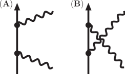
Figure 1: Tree diagrams for muon Compton scattering.

The advantage of working with the dimensionless variables $x$ and $y$ shows up already when evaluating the Born terms. The two tree diagrams shown in Fig. 1 lead to the following simple polynomial expressions:

$$A\otimes A=2x-xy+4\,,\quad A\otimes B=B\otimes A=x+y+4\,,\quad B\otimes B=2y-xy+4\,.$$ (3)

When inserted into eq.(2), they produce the well-known Klein-Nishina cross section. In the center-of-mass frame the variables $x$ and $y$ are the related to the total center-of-mass energy $\sqrt{s}$ and the cosine of the scattering angle $\cos\theta_{\rm cm}$ in the following way:

$$x=\bigg{(}{\sqrt{s}\over m}\bigg{)}^{2}-1\,,\qquad y=-{x\over 2(1+x)}(2+x+x\cos\theta_{\rm cm})\,.$$ (4)

In the laboratory frame, on the other hand, $x$ and $y$ are directly proportional to the energies $E_{\gamma}$ and $E^{\prime}_{\gamma}$ of the incoming and outgoing photon:

$$x={2E_{\gamma}\over m}\,,\qquad y=-{2E^{\prime}_{\gamma}\over m}\,,\qquad 1-\cos\theta_{\rm lab}=-2\bigg{(}{1\over x}+{1\over y}\bigg{)}\,,$$ (5)

with the scattering angle $\theta_{\rm lab}$ fixed by them. In the physical region the inequalities, $x\geq 0$ and $-x\leq y\leq-x/(1+x)\leq 0$, hold. The radiative corrections to muon-pair annihilation $\mu^{+}\mu^{-}\to\gamma\gamma$ are obtained by specifying $x$ and $y$ in eq.(2) for that (crossed) reaction.

2.1 Evaluation of one-photon loop diagrams

In this section, we present analytical expressions (of order $\alpha$) for the interference terms between the one-photon loops diagrams and the tree diagrams for muon Compton scattering. We use the method of dimensional regularization to treat both ultraviolet and infrared divergencies (where the latter are caused by the masslessness of the photon). The method consists in calculating loop integrals in $d$ spacetime dimensions and expanding the results around $d=4$. Divergent pieces of one-loop integrals generically show up in form of the composite constant:

$$\xi={1\over d-4}+{1\over 2}(\gamma_{E}-\ln 4\pi)+\ln{m\over\mu}\,,$$ (6)

containing a simple pole at $d=4$. In addition, $\gamma_{E}=0.5772\dots$ is the Euler-Mascheroni number and $\mu$ an arbitrary mass scale introduced in dimensional regularization in order to keep the mass dimension of the loop integrals independent of $d$. Ultraviolet (UV) and infrared (IR) divergencies are distinguished by the feature of whether the condition for convergence of the $d$-dimensional integral is $d<4$ or $d>4$. We discriminate them in the notation by putting appropriate subscripts, i.e. $\xi_{UV}$ and $\xi_{IR}$. In order to simplify all calculations, we employ the Feynman gauge where the photon propagator is directly proportional to the Minkowski metric tensor $g^{\mu\nu}$. Let us now enumerate the analytical results as they emerge from the four classes of one-photon loop diagrams shown in Figs. 2,3.

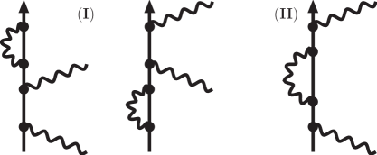
Figure 2: One-photon loop diagrams, (I) and (II), for muon Compton scattering.

Class I. These photon-loop diagrams introduce the wavefunction renormalization factor $Z_{2}-1=\alpha(2\xi_{IR}+\xi_{UV}-2)/2\pi$ [16] of the muon and the pertinent interference terms with the (direct and crossed) tree diagrams read:

$${\rm I}\otimes A={\alpha\over 2\pi}\bigg{\{}(2\xi_{IR}+\xi_{UV}-2)\bigg{(}2-y+{4\over x}\bigg{)}-y\bigg{\}}\,,$$ (7)

$${\rm I}\otimes B={\alpha\over 2\pi}\bigg{\{}(2\xi_{IR}+\xi_{UV}-2)\,{x+y+4\over x}-{y\over 2}\bigg{\}}\,.$$ (8)

The additive terms, $-y$ and $-y/2$, come from evaluating the Dirac-traces and Lorentz-index contractions consistently in $d$ spacetime dimensions and expanding the results around $d=4$. Within dimensional regularization it is crucial to follow this prescription in order to recover the correct low-energy limit $(k_{1},k_{2}\to 0)$ for Compton scattering, namely the non-renormalization of the Thomson amplitude [7].

Class II. This photon-loop diagram involves the off-shell fermion selfenergy subtracted by the mass shift. The corresponding interference terms with the tree diagrams $A$ and $B$ read:

$${\rm II}\otimes A = {\alpha\over 4\pi x}\bigg{\{}2\xi_{UV}(2x-xy+4)-xy-5x+{3x\over x+1}$$ (9)

$$+\bigg{[}11x-xy+3y-26+{13-3y\over x+1}-{3\over(x+1)^{2}}\bigg{]}\ln(-x)\bigg{\}}\,,$$

$${\rm II}\otimes B = {\alpha\over 2\pi x}\bigg{\{}\xi_{UV}(x+y+4)-{xy\over 2}+{x(y-1)\over x+1}$$ (10)

$$+\bigg{[}{3y-7\over x+1}+{1-y\over(x+1)^{2}}-x-4y-2\bigg{]}\ln(-x)\bigg{\}}\,.$$

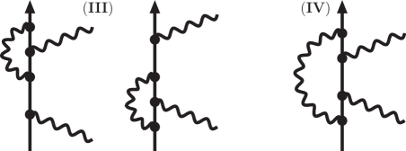
Figure 3: One-photon loop diagrams, (III) and (IV), for muon Compton scattering.

Class III. These photon-loop diagrams involve the half off-shell vertex correction. Both of them contribute equally and the pertinent interference terms with the tree diagrams read:

$${\rm III}\otimes A = {\alpha\over 2\pi x}\bigg{\{}2\xi_{UV}(xy-2x-4)+2x^{2}+4xy+7x+15+{1\over x+1}$$ (11)

$$+\bigg{[}7-10x-x^{2}-2y(x+1)+{2y-8\over x+1}+{1\over(x+1)^{2}}\bigg{]}\ln(-x)$$

$$-4\bigg{(}2+x+y+{4\over x}\bigg{)}\bigg{[}{\rm Li}_{2}(x+1)-{\pi^{2}\over 6}\bigg{]}\bigg{\}}\,,$$

$${\rm III}\otimes B = {\alpha\over 2\pi x}\bigg{\{}-2\xi_{UV}(x+y+4)-3y^{2}-2xy-8y-{2y\over x}(8+y)-{x^{2}\over x+1}$$ (12)

$$+\bigg{[}4x+3xy+13y+3y^{2}+5-{1\over(x+1)^{2}}+{12-5y\over x+1}+{2y\over x}(8+y)\bigg{]}\ln(-x)$$

$$+\bigg{[}3y+1+{2y\over x}(3+y)+{y\over x^{2}}(8+y)\bigg{]}\bigg{[}2{\rm Li}_{2}(x+1)-{\pi^{2}\over 3}\bigg{]}\bigg{\}}\,,$$

where Li${}_{2}(x)=\sum_{n=1}^{\infty}n^{-2}x^{n}=x\int_{1}^{\infty}d\xi[\xi(\xi-x)]^{-1}\ln\xi$ denotes the conventional dilogarithmic function. A particular part of the vertex corrections (on the mass-shell) is the muon anomalous magnetic moment $\kappa=\alpha/2\pi$. Taken by its own the anomalous magnetic moment leads (via an appropriate derivative-coupling vertex) to the contributions:

$$\kappa\otimes A=-{3\alpha\over 4\pi}(2x+y)\,,\qquad\kappa\otimes B={\alpha\,y\over 4\pi x}(4x+y)\,.$$ (13)

By comparing with the complete (off-shell) vertex corrections written in eqs.(11,12) one notices that there is no obvious way to localize therein the anomalous magnetic moment contributions. On-shell and off-shell effects from the photon-loop appear to be inseparably mixed in the interference terms III$\,\otimes\,A$ and III$\,\otimes\,B$.

Class IV. The evaluation the photon-loop box diagram is most challenging and one finds for its interference terms with the tree diagrams $A$ and $B$:

$${\rm IV}\otimes A = {\alpha\over 2\pi}\Bigg{\{}{(8+3x)y\over x+y}-4-4y+\bigg{[}x+2y+{3x\over x+1}\bigg{]}\ln(-x)$$ (14)

$$+\bigg{[}2+y+{4\over x}(y-1)\bigg{]}\bigg{[}{\rm Li}_{2}(x+1)-{\pi^{2}\over 6}\bigg{]}+4\xi_{IR}\bigg{(}y-2-{4\over x}\bigg{)}$$

$$\times{2+x+y\over\sqrt{4+x+y}}\,L(x+y)+{2L(x+y)\over\sqrt{4+x+y}}\bigg{[}y-x-x^{2}-2xy+{4x(4-y)\over x+y}$$

$$+\bigg{(}xy+y^{2}-2x-12-{8\over x}(2+y)\bigg{)}\ln(-x)\bigg{]}+\bigg{(}4-2y-xy-y^{2}-{4xy\over x+y}\bigg{)}$$

$$\times L^{2}(x+y)+{2+x+y\over h_{+}-h_{-}}\bigg{\{}\bigg{(}y-2-{4\over x}\bigg{)}\bigg{[}{\rm Li}_{2}(w)-{\rm Li}_{2}(1-w)$$

$$+{1\over 2}\ln^{2}w-{1\over 2}\ln^{2}(1-w)\bigg{]}+\bigg{(}{4\over x}+1-{y\over 2}\bigg{)}\Big{[}{\rm Li}_{2}(h_{+})-{\rm Li}_{2}(h_{-})\Big{]}\bigg{\}}\Bigg{\}}\,,$$

$${\rm IV}\otimes B = {\alpha\over 2\pi}\Bigg{\{}{x\over x+1}+{4y\over x}(y-1)+{y\over x+y}(8+x-2y)$$ (15)

$$+\bigg{[}{4y\over x}(1-y)-4y-1-{1\over(x+1)^{2}}+{6-4y\over x+1}\bigg{]}\ln(-x)$$

$$+\bigg{[}x+y-1-{4+y\over x}+{2y\over x^{2}}(1-y)\bigg{]}\bigg{[}2{\rm Li}_{2}(x+1)-{\pi^{2}\over 3}\bigg{]}$$

$$-{4\xi_{IR}\over x}(2+x+y)\sqrt{4+x+y}\,L(x+y)+{2L(x+y)\over\sqrt{4+x+y}}$$

$$\times\bigg{[}x+7y-16+2xy+3y^{2}+{4x(4-y)\over x+y}+\bigg{(}2(x+y)^{2}-24$$

$$-{2\over x}(8+6y+y^{2})\bigg{)}\ln(-x)\bigg{]}+\bigg{(}4+2x-2(x+y)^{2}+{4y^{2}\over x+y}\bigg{)}$$

$$\times L^{2}(x+y)+{1\over x(h_{+}-h_{-})}\bigg{\{}(2+x+y)(4+x+y)$$

$$\times\bigg{[}{\rm Li}_{2}(1-w)-{\rm Li}_{2}(w)+{1\over 2}\ln^{2}(1-w)-{1\over 2}\ln^{2}w\bigg{]}$$

$$+\Big{(}8+12x-x^{3}+2y(3-x^{2})+y^{2}(1-x)\Big{)}\Big{[}{\rm Li}_{2}(h_{+})-{\rm Li}_{2}(h_{-})\Big{]}\bigg{\}}\Bigg{\}}\,.$$

Here, we have introduced the frequently occurring logarithmic loop function:

$$L(x)={1\over\sqrt{x}}\ln{\sqrt{4+x}+\sqrt{x}\over 2}\,,$$ (16)

and the auxiliary variables:

$$w={1\over 2}\bigg{(}1-\sqrt{{x+y\over 4+x+y}}\,\bigg{)}\,,\qquad h_{\pm}={1\over 2}\Big{[}-x-y\pm\sqrt{(x+y)(4+x+y)}\,\Big{]}\,.$$ (17)

It is remarkable that only one single loop integral involving four propagators contributes at the end to the interference terms IV$\,\otimes\,A$ and IV$\,\otimes\,B$. This (scalar) loop integral is infrared divergent and it can actually be solved in terms of logarithms ($L(x+y),\ln(-x),\ln^{2}w,\ln^{2}(1-w)$) and dilogarithms (${\rm Li}_{2}(1-w),{\rm Li}_{2}(w),{\rm Li}_{2}(h_{\pm})$). As an immediate check, one verifies that the ultraviolet divergent terms proportional to $\xi_{UV}$ cancel out in the sums (I+II+III)$\,\otimes\,A$ and (I+II+III)$\,\otimes\,B$.

2.2 Infrared finiteness

In the next step we have to consider the infrared divergent terms proportional to $\xi_{IR}$. Inspection of eqs.(7,8,14,15) reveals that these scale with the Born terms $A\otimes A/x$ and $A\otimes B/x$ given in eq.(3). As a consequence of that feature, the infrared divergent loop corrections multiply differential cross section $d\sigma/d\Omega_{\rm cm}$ at leading order by a ($x\leftrightarrow y$ crossing-symmetric) factor:

$$\delta_{\rm virt}^{(\rm IR)}={2\alpha\over\pi}\Bigg{[}1-{4+2x+2y\over\sqrt{4+x+y}}\,L(x+y)\Bigg{]}\,\xi_{IR}\,.$$ (18)

The (unphysical) infrared divergence $\xi_{IR}$ gets canceled at the level of the (measurable) cross section by the contributions of soft photon bremsstrahlung. In its final effect, the (single) soft photon radiation multiplies the tree level cross section $d\sigma/d\Omega_{\rm cm}$ by a factor [7, 17]:

$$\delta_{\rm soft}=\alpha\,\mu^{4-d}\!\!\int\limits_{|\vec{l}\,|<\lambda}\!\!{d^{d-1}l\over(2\pi)^{d-2}\,l_{0}}\bigg{\{}{2p_{1}\cdot p_{2}\over p_{1}\cdot l\,p_{2}\cdot l}-{m^{2}\over(p_{1}\cdot l)^{2}}-{m^{2}\over(p_{2}\cdot l)^{2}}\bigg{\}}\,,$$ (19)

which depends on a small energy cut-off $\lambda$. Working out this momentum space integral by the method of dimensional regularization (with $d>4$) one finds that the infrared divergent correction factor $\delta_{\rm virt}^{(\rm IR)}\sim\xi_{IR}$ in eq.(18) gets eliminated and the following finite radiative correction factor remains:

$$\delta_{\rm real}^{(\rm cm)} = {\alpha\over\pi}\Bigg{\{}\bigg{[}2-{8+4x+4y\over\sqrt{4+x+y}}\,L(x+y)\bigg{]}\ln{m\over 2\lambda}+{x+2\over x}\ln(x+1)$$ (20)

$$\qquad-\int_{0}^{1/2}\!\!d\tau\,{(x+2)(2+x+y)\over[1+(x+y)\tau(1-\tau)]\sqrt{W}}\ln{x+2+\sqrt{W}\over x+2-\sqrt{W}}\Bigg{\}}\,,$$

with the abbreviation $W=x^{2}-4(x+1)(x+y)\tau(1-\tau)$. We note that the terms beyond those proportional to $\ln(m/2\lambda)$ are specific for the evaluation of the soft photon correction factor $\delta_{\rm soft}$ in the $\mu^{-}\gamma$ center-of-mass frame with $\lambda$ an infrared cut-off therein.

Having the analytical results at hand, one can show that both the virtual and the real radiative corrections vanish as one approaches (at fixed scattering angle $\theta_{\rm cm}$) the Compton threshold, $\sqrt{s}\to m$ or $x\to 0$. This non-renormalization of the Thomson cross section $d\sigma/d\Omega_{\rm cm}=\alpha^{2}(1+\cos^{2}\theta_{\rm cm})/2m^{2}$ serves as an important check on the method of dimensional regularization where spin and polarization sums are extended from $4$ to $d$ spacetime dimensions.

2.3 Results and discussion

We are now in the position to present numerical results for the radiative corrections to muon Compton scattering $\mu^{-}\gamma\to\mu^{-}\gamma$. The complete radiative correction factor is $\delta_{\rm real}$ written in eq.(20) plus the sum of all interference terms (second line in eq.(2)) divided by the Born terms (first line in eq.(2)). First, it is important to note that our calculation (which employs dimensional regularization to treat both ultraviolet and infrared divergent loop integrals) confirms the absolute correctness of the expression written in eq.(52.12) of ref.[13] for the radiative corrections to spin-1/2 Compton scattering. Fig. 4 shows in percent the total radiative correction factor for four selected center-of-mass energies $\sqrt{s}=(2,3,4,5)m$. The detection threshold for soft photons has been set to the value $\lambda=3.8\,$MeV. One observes that the radiative corrections become maximal in backward directions $\cos\theta_{\rm cm}\simeq-1$, reaching values up to $-3\%$ at $\sqrt{s}=5m$. In Fig. 5 we show for comparison the radiative corrections to pion Compton scattering [7] (for an equivalent infrared cut-off of $\lambda=5\,$MeV). One notices that the overall magnitude and angular dependence of the radiative corrections are very similar in both cases. Interestingly, the dip in backward directions is more pronounced in the spin-0 case.

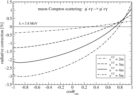
Figure 4: One-photon loop radiative corrections to muon Compton scattering.

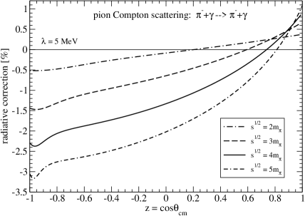
Figure 5: Radiative corrections for pion Compton scattering $\pi^{-}\gamma\to\pi^{-}\gamma$.

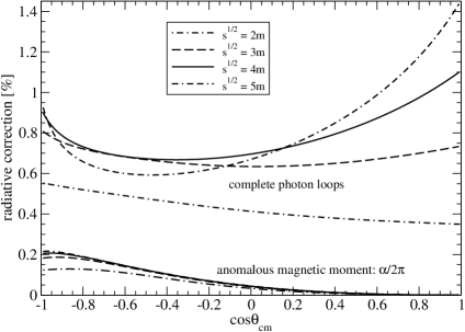
Figure 6: Effect of anomalous magnetic moment $\kappa=\alpha/2\pi$ compared to the complete photon-loops.

Next, we discuss the role of the muon anomalous magnetic moment $\kappa=\alpha/2\pi$. As a radiative correction it represents the on-shell part of the vertex corrections generated by the photon-loop diagrams of class III (see Fig. 3). The comparison made in Fig. 6 informs us that the muon anomalous magnetic moment $\kappa=\alpha/2\pi$ provides only a very small portion of the complete radiative corrections arising from the full set of photon-loop diagrams. Most noticeably, the contribution of the anomalous magnetic moment vanishes in forward directions $\cos\theta_{\rm cm}\simeq 1$, whereas the complete radiative corrections grow strongly with the center-of-mass energy $\sqrt{s}$ in that region. Note that we have omitted the soft photon contribution $\delta_{\rm real}^{(\rm cm)}$ in the comparison shown in Fig. 6.

The radiative corrections in forward direction $\cos\theta_{\rm cm}=1$ are of particular interest, because for this kinematical situation the soft bremsstrahlung contribution $\delta_{\rm real}^{(\rm cm)}$ vanishes identically. The soft photon emission before and after the Compton scattering process interfere in this case destructively with each other. After taking carefully the forward limit $y\to-x$ of all terms calculated in section 2.1, we get for the radiative corrections to muon Compton scattering in forward direction:

$$\delta_{0}(x) = {\alpha\over 2\pi}\bigg{\{}{4-3x^{2}\over x^{2}-1}+{x^{4}-3x^{2}\over(x^{2}-1)^{2}}\ln x+{\pi^{2}\over 3x^{2}}(x^{2}-8)$$ (21)

$$+{8+4x-x^{2}\over x^{2}}\,{\rm Re}\,{\rm Li}_{2}(x+1)+{8-4x-x^{2}\over x^{2}}\,{\rm Li}_{2}(1-x)\bigg{\}}\,.$$

The dependence of this function on the center-of-mass energy $\sqrt{s}=m\sqrt{x+1}$ is reproduced by the full curve in Fig. 7. Its asymptotic behavior is $(\alpha/2\pi)\ln^{2}x$. The dashed curve in Fig. 7 shows for comparison the same quantity for Compton scattering off a (point-like) spin-0 particle. Using the analytical results in section 3 of ref.[7] one deduces the expression:

$$\delta_{0}(x)^{\rm spin-0}={2\alpha\over\pi}\bigg{\{}{x^{2}\ln x\over x^{2}-1}-{2\pi^{2}\over 3x^{2}}-1+{2+x\over x^{2}}\,{\rm Re}\,{\rm Li}_{2}(x+1)+{2-x\over x^{2}}\,{\rm Li}_{2}(1-x)\bigg{\}}\,,$$ (22)

for the radiative corrections to pion Compton scattering in forward direction. The asymptotic behavior $(2\alpha/\pi)\ln x$ in the spin-0 case turns out to be weaker than for the muon. Presumably, this difference has its origin in the additional magnetic coupling of the photon to a (point-like) spin-1/2 particle.

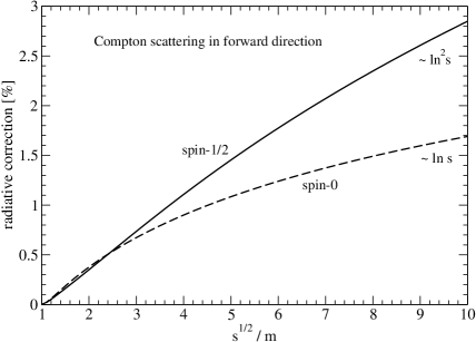
Figure 7: Radiative correction to muon and pion Compton scattering in forward direction.

3 Radiative corrections to muon-nucleus bremsstrahlung

In this section we extend our calculation of radiative corrections to the muon-nucleus brems- strahlung process $\mu^{-}Z\to\mu^{-}Z\gamma$. In the one-photon exchange approximation a virtual Coulomb photon couples to the heavy nucleus of charge $Z$ and the bremsstrahlung process is governed by the virtual muon Compton scattering: $\mu^{-}(p_{1})+\gamma^{*}_{0}(q)\to\mu^{-}(p_{2})+\gamma(k,\epsilon)$. The in- and out-going four-momenta of that subprocess give rise to the following kinematical variables:

$$s=(p_{1}+q)^{2}=(p_{2}+k)^{2}=m^{2}(x+1)\,,\qquad u=(p_{1}-k)^{2}=(p_{2}-q)^{2}=m^{2}(y+1)\,,$$ (23)

$$E_{1}=m\,e_{1}\,,\qquad E_{2}=m\,e_{2}\,,\qquad q^{2}=-m^{2}Q\,,\qquad q_{0}=0\,,$$ (24)

where we have also noted that the extremely small recoil energy $-q_{0}=\vec{q}\,^{2}/2M_{\rm nucl}\approx 0$ of the nucleus can be neglected. In the following it will be most advantageous to work with the five independent dimensionless variables $e_{1},e_{2},x,y,Q$. The unpolarized (fivefold) differential cross section for muon-nucleus bremsstrahlung in the laboratory frame reads [15]:

$${d^{5}\sigma\over d\omega d\Omega_{\gamma}d\Omega_{\mu}}={Z^{2}\alpha^{3}\omega|\vec{p}_{2}|\over\pi^{2}|\vec{p}_{1}||\vec{q}\,|^{4}}\,H\,,$$ (25)

with $\omega=k_{0}=m(e_{1}-e_{2})$, $|\vec{p}_{j}|=m\sqrt{e_{j}^{2}-1}$, $|\vec{q}\,|=m\sqrt{Q}$ and $H$ is the squared amplitude summed over muon spin and photon polarization states. This sum is carried out most conveniently via a Dirac-trace and a contraction with the (negative) Minkowski metric tensor, $-{1\over 8}{\rm tr}[(/\!\!\!p_{2}+m)O^{\nu}(/\!\!\!p_{1}+m){\overline{O}}_{\nu}]$. In that procedure the virtual Coulomb photon is given the polarization four-vector $v^{\mu}=(1,\vec{0}\,)$ which provides in the form of Lorentz-scalar products the muon energies $E_{1}=m\,e_{1}$ and $E_{2}=m\,e_{2}$ as further independent variables.

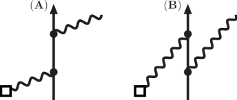
Figure 8: Tree diagrams for virtual muon Compton scattering.

The direct and crossed tree diagrams for virtual muon Compton scattering (named again $A$ and $B$) are shown in Fig. 8. The open square in the left lower corner should symbolize the heavy nucleus to which the virtual Coulomb photon $\gamma_{0}^{*}$ couples. The contribution of these two tree diagrams to the squared amplitude $H$ has the form:

$$H_{\rm tree}=\bigg{(}{A\over x}+{B\over y}\bigg{)}\otimes\bigg{(}{A\over x}+{B\over y}\bigg{)}\,,$$ (26)

with

$$A\otimes A=2e_{1}^{2}(x-2)-2e_{1}e_{2}\,x+Q+{xy\over 2}\,,$$ (27)

$$A\otimes B=e_{1}e_{2}(x+y-4)-e_{1}^{2}(Q+y)-e_{2}^{2}(Q+x)+{Q\over 2}(2+Q+x+y)\,,$$ (28)

$$B\otimes B=2e_{2}^{2}(y-2)-2e_{1}e_{2}\,y+Q+{xy\over 2}\,,$$ (29)

where the product symbol $\otimes$ designates again the interference term between (the T-matrices from) two diagrams with the sums over muon spins and photon polarizations already carried out. As it is written here in eqs.(26-29) the term $H_{\rm tree}$ reproduces to the familiar Bethe-Heitler cross section [15] (now reexpressed in terms of the independent variables $e_{1},e_{2},x,y,Q$). We note as an aside that for a spin-0 particle (e.g. a pion) $H_{\rm tree}$ reduces to a much simpler form:

$$H_{\rm tree}^{(\rm spin-0)}=-4\bigg{(}{e_{1}\over x}+{e_{2}\over y}\bigg{)}^{2}-{4e_{1}e_{2}Q\over xy}-1\,.$$ (30)

The radiative corrections of order $\alpha$ to virtual muon Compton scattering $\mu^{-}\gamma^{*}_{0}\to\mu^{-}\gamma$ can be summarized by the contribution:

$$H_{\rm loop}=2\,{\rm Re}\bigg{[}\Big{(}{\rm I+II+III+IV+V}\Big{)}\otimes\bigg{(}{A\over x}+{B\over y}\bigg{)}+(x\leftrightarrow y,\,e_{1}\leftrightarrow-e_{2})\bigg{]}\,,$$ (31)

where I, II, III, IV, V denote the five classes of one-photon loop diagrams shown in Figs. 9,10. The symmetrization prescription $+(x\leftrightarrow y,\,e_{1}\leftrightarrow-e_{2})$ supplies the additional contributions from the crossed one-photon loop diagrams. These are obtained by interchanging the coupling vertex of the left and the right photon line in the diagrams of Figs. 9,10.

3.1 Evaluation of one-photon loop diagrams

In this section we collect the analytical expressions for the interference terms between one-photon loop diagrams and tree diagrams for virtual muon Compton scattering. Such a direct (diagrammatic) calculation of the radiative corrections to bremsstrahlung has been deferred in ref.[10, 11] as being too difficult and instead the so-called mass operator method [18] has been used.

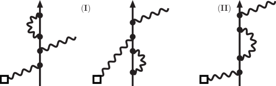
Figure 9: One-photon loop diagrams, (I) and (II), for virtual muon Compton scattering.

Class I. These photon-loop diagrams introduce the wavefunction renormalization factor $Z_{2}-1$ and the pertinent interference terms with the tree diagrams ($A$ and $B$) read:

$${\rm I}\otimes A={\alpha\over 2\pi}\bigg{\{}(2\xi_{IR}+\xi_{UV}-2){A\otimes A\over x}+e_{1}^{2}-e_{1}e_{2}+{y\over 4}\bigg{\}}\,,$$ (32)

$${\rm I}\otimes B={\alpha\over 4\pi x}\bigg{\{}2(2\xi_{IR}+\xi_{UV}-2)A\otimes B+e_{1}e_{2}(x+y)-e_{1}^{2}\,y-e_{2}^{2}\,x-Q(e_{1}-e_{2})^{2}+{xy\over 2}\bigg{\}}\,,$$ (33)

with $A\otimes A$ and $A\otimes B$ given in eqs.(27,28).

Class II. This photon-loop diagram involves the off-shell selfenergy subtracted by the mass shift and the corresponding interference terms with the tree diagrams read:

$${\rm II}\otimes A = {\alpha\over 4\pi x}\bigg{\{}2\xi_{UV}A\otimes A+{x\over x+1}\bigg{(}2e_{1}^{2}-{Q\over 2}+x\bigg{)}+\Big{[}4e_{1}^{2}(8+8x+x^{3})$$ (34)

$$+(4e_{1}e_{2}-y)(2x+x^{2}-x^{3})-Q(8+10x+x^{2})-4x^{2}-6x^{3}\Big{]}{\ln(-x)\over 2(x+1)^{2}}\bigg{\}}\,,$$

$${\rm II}\otimes B = {\alpha\over 4\pi x}\bigg{\{}2\xi_{UV}A\otimes B+{1\over 2(x+1)}\Big{[}2e_{1}e_{2}(2Q+x+2Qx+y)-2e_{1}^{2}(Q+y)$$ (35)

$$+2e_{2}^{2}(x-Q)-Qx(3+Q+x+y)+x^{2}y\Big{]}+\bigg{[}{xy\over 2}(3x+2)$$

$$-e_{2}^{2}x^{2}(x+2)+\bigg{(}{2e_{1}^{2}-Q\over 2}(Q+y)-e_{1}e_{2}y+e_{2}^{2}Q\bigg{)}(4+4x-x^{2})$$

$$+e_{1}e_{2}(16+20x+4x^{2}+x^{3})+{Q\over 2}(x^{3}+x^{2}-10x-8)\bigg{]}{\ln(-x)\over(x+1)^{2}}\bigg{\}}\,.$$

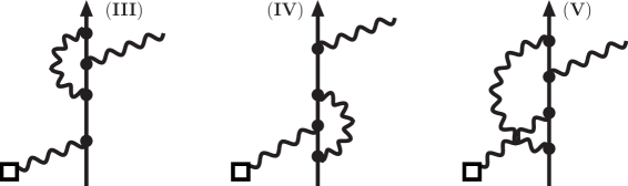
Figure 10: One-photon loop diagrams, (III), (IV) and (V), for virtual muon Compton scattering.

Class III. The vertex correction to the (upper) real photon emission introduces loop functions that depend only on the variable $x$ (related to $s=(p_{2}+k)^{2}$). The pertinent interference terms with the tree diagrams ($A$ and $B$) read:

$${\rm III}\otimes A = {\alpha\over 4\pi x}\bigg{\{}-2\xi_{UV}A\otimes A-x^{2}-18e_{1}^{2}+{9Q+1\over 2}+{4e_{1}^{2}-1-Q\over 2(x+1)}$$ (36)

$$+{x\over 2}(12e_{1}e_{2}-4e_{1}^{2}-2Q-3y-1)+\bigg{[}Q(x^{2}-2x-2)+x^{3}+6x^{2}$$

$$+4x+4e_{1}^{2}(x^{2}+8x+6)+(2y-8e_{1}e_{2})(x^{2}+3x+2)\bigg{]}{x\ln(-x)\over 2(x+1)^{2}}$$

$$+\bigg{[}8e_{1}^{2}-8e_{1}e_{2}+x+2y+{4\over x}(4e_{1}^{2}-Q)\bigg{]}\bigg{[}{\rm Li}_{2}(x+1)-{\pi^{2}\over 6}\bigg{]}\bigg{\}}\,,$$

$${\rm III}\otimes B = {\alpha\over 4\pi x}\bigg{\{}-2\xi_{UV}A\otimes B+{x\over 2}(1+Q+2y-2e_{1}e_{2})+{1\over 2}(1+Q^{2}+3y^{2})$$ (37)

$$+{1\over x+1}\bigg{[}e_{1}^{2}(Q-y)+e_{1}e_{2}(Q+3)-{1\over 2}(Q+1)^{2}\bigg{]}-4e_{2}^{2}+Q+2y+2Qy$$

$$+{y\over x}(20e_{1}^{2}-4e_{1}e_{2}-4Q+y)+e_{1}^{2}(Q+y)+e_{1}e_{2}(1-6y-3Q)$$

$$+\bigg{[}{y\over x}(4e_{1}e_{2}+4Q-y-20e_{1}^{2})+{x\over 2}(2e_{1}e_{2}+2e_{2}^{2}-2-Q-3y)-{y\over 2}(7+3y)$$

$$+{1\over 2(x+1)^{2}}\Big{(}2e_{1}^{2}(Q-y)+2e_{1}e_{2}(3+Q)-(Q+1)^{2}\Big{)}+{1\over x+1}\bigg{(}2e_{1}^{2}(y-3Q)$$

$$+e_{1}e_{2}(5y-Q-17)+1-e_{2}^{2}+{3\over 2}(3Q+y)+Q(3Q+y-5e_{2}^{2})\bigg{)}-2Qy$$

$$-e_{1}^{2}(Q+y)+e_{1}e_{2}(2Q+5y-6)+e_{2}^{2}(5+Q)+{1\over 2}(Q-Q^{2}-1)\bigg{]}\ln(-x)$$

$$+\bigg{[}{1\over x}\Big{(}2e_{1}e_{2}(Q-2+4y)-2e_{1}^{2}(Q+3y)+4e_{2}^{2}-2y-Qy-2y^{2}\Big{)}$$

$$+{y\over x^{2}}(4e_{1}e_{2}+4Q-y-20e_{1}^{2})+2e_{1}e_{2}-2y-1\bigg{]}\bigg{[}{\rm Li}_{2}(x+1)-{\pi^{2}\over 6}\bigg{]}\bigg{\}}\,.$$

Class IV. The vertex correction to the (lower) virtual photon absorption introduces loop functions that depend on two variables, $x$ and $Q$. The pertinent interference terms with the tree diagrams ($A$ and $B$) read:

$${\rm IV}\otimes A = {\alpha\over 4\pi x}\Bigg{\{}-2A\otimes A\,\bigg{[}\xi_{UV}+\int_{0}^{1}\!\!da\!\int_{0}^{1}\!\!db\,b\ln K(a,b;x,Q)\bigg{]}+e_{1}^{2}(6-5x)+5e_{1}e_{2}x$$ (38)

$$-{1\over 4}(6Q+5xy)+\int_{0}^{1}\!\!da\!\int_{0}^{1}\!\!db\,{1\over K(a,b;x,Q)}\bigg{\{}2e_{1}^{2}(8+4Q-Qx+xy)$$

$$+2e_{1}e_{2}x(2+Q+x)-2Q^{2}-Q(4+3x+xy)-x(2x+y+xy)$$

$$+\Big{[}2e_{1}^{2}(Qx+4x-8-4Q-xy)-2e_{1}e_{2}x(4+Q+x)+Q(8+3x+xy)$$

$$+2Q^{2}+x(2x+3y+xy)\Big{]}b+\Big{[}2e_{1}e_{2}(Q-x)-2e_{1}^{2}(Q+y)+2Q+xy\Big{]}x\,ab$$

$$+\Big{[}2e_{1}^{2}(4Q-Qx+xy)+(2e_{1}e_{2}x-2Q-xy)(Q+x)\Big{]}ab^{2}$$

$$-\Big{[}4e_{1}^{2}(2+x)+2Q+xy\Big{]}b^{2}+\Big{[}4e_{1}^{2}(x-2)-4e_{1}e_{2}x+2Q+xy\Big{]}Q\,a^{2}b^{2}\bigg{\}}\Bigg{\}}\,,$$

$${\rm IV}\otimes B = {\alpha\over 4\pi x}\Bigg{\{}-2A\otimes B\,\bigg{[}\xi_{UV}+\int_{0}^{1}\!\!da\!\int_{0}^{1}\!\!db\,b\ln K(a,b;x,Q)\bigg{]}+{5e_{1}^{2}\over 2}(Q+y)$$ (39)

$$+{5e_{2}^{2}\over 2}(Q+x)+{e_{1}e_{2}\over 2}(12-4Q-5x-5y)-{xy\over 2}-{3Q\over 4}(2+Q+x+y)$$

$$+\int_{0}^{1}\!\!da\!\int_{0}^{1}\!\!db\,{1\over K(a,b;x,Q)}\bigg{\{}2e_{1}^{2}(2+Q)(Q+y)+2e_{2}^{2}(2Q+Q^{2}+2Qx+x^{2})$$

$$+2e_{1}e_{2}(8+4Q+2x-2y-Qy+xy)-Q^{3}+xy-Q^{2}(4+2x+y)$$

$$-Q(4+3x+x^{2}+2y+xy)+\Big{[}Q^{3}-xy-2e_{1}^{2}(2+Q)(Q+y)$$

$$+2e_{1}e_{2}(2x+2y-8-2Q+Qy-xy)-2e_{2}^{2}(4Q+Q^{2}+2x+2Qx+x^{2})$$

$$+Q^{2}(6+2x+y)+Q(8+5x+x^{2}+4y+xy)\Big{]}\,b+\Big{[}Q(2+Q+x+y)$$

$$-2e_{2}^{2}(Q+x)-2e_{1}e_{2}(Q+y)\Big{]}\,x\,ab+\Big{[}2e_{1}^{2}Q(Q+y)+2e_{1}e_{2}(4Q-Qy+xy)$$

$$+2e_{2}^{2}(Q+x)^{2}-Q^{3}-Qx(2+x+y)-Q^{2}(2+2x+y)\Big{]}\,ab^{2}+\Big{[}2e_{2}^{2}(Q+x)$$

$$-2e_{1}e_{2}(4+2Q+3x-y)-2e_{1}^{2}(Q+y)-Q^{2}-Q(2+x+y)\Big{]}\,b^{2}+Q\,a^{2}b^{2}$$

$$\times\Big{[}2e_{1}e_{2}(x+y-4)-2e_{1}^{2}(Q+y)-2e_{2}^{2}(Q+x)+Q(Q+2+x+y)\Big{]}\bigg{\}}\Bigg{\}}\,,$$

with the cubic polynomial $K(a,b;x,Q)=b+xa(b-1)+Qa(1-a)b$ in two Feynman parameters $a,b$. In the physical region, $x>0$ and $Q>0$, the integrals involving $1/K(a,b;x,Q)$ are singular and in fact they become complex-valued. In order to compute their real parts (which are only of relevance according to eq.(31)), one performs the Feynman parameter integral $\int_{0}^{1}db$ analytically and converts the occurring (complex) logarithm $\ln(-ax)$ into $\ln(ax)$. The remaining integral $\int_{0}^{1}da$ is free of poles and therefore unproblematic for a numerical treatment. For the contributions of the crossed photon-loops, where $x>0$ is replaced by $y<0$, the two-parameter integrals in eqs.(38,39) are real-valued and can be evaluated numerically as they stand.

On the mass-shell the vertex corrections arising from the diagrams III and IV reduce to the anomalous magnetic moment $\kappa=\alpha/2\pi$. This piece alone leads to the following interference terms with the tree diagrams:

$$\kappa\otimes A={\alpha\over 4\pi}\bigg{\{}3e_{1}^{2}-3e_{1}e_{2}+{Q\over 2x}(x+4)+{1\over 4}(7x+5y)\bigg{\}}\,,$$ (40)

$$\kappa\otimes B = {\alpha\over 4\pi x}\bigg{\{}e_{1}e_{2}(4Q+x+2y)-e_{1}^{2}(Q+2y)-e_{2}^{2}(3Q+x)$$ (41)

$$\qquad\,\,+Q\bigg{(}2+{x\over 2}+y\bigg{)}+Q^{2}-{y\over 4}(3x+y)\bigg{\}}\,.$$

Class V. The box diagram is most tedious to evaluate. A good fraction of the occurring loop integrals with three and four propagators can be still be solved in closed analytical form, while the remaining ones have to be represented as parametric integrals. Putting all pieces together, we find the following rather lengthy expressions for the interference terms of the photon-loop diagram V with the tree diagrams ($A$ and $B$):

$${\rm V}\otimes A = {\alpha\over 4\pi}\Bigg{\{}\Big{[}4e_{1}^{2}(Q-4+3x+2y)+4e_{1}e_{2}(4-3Q-4x-3y)+(x+y)(2+x+y)$$ (42)

$$+Q(2Q+6+3x+2y)\Big{]}{1\over x+y}\Big{[}(Q+x+y)\,L^{2}(Q+x+y)-Q\,L^{2}(Q)\Big{]}$$

$$+\Big{[}8e_{1}^{2}(2-2x-y)+4e_{1}e_{2}(4x-4+3y)+4e_{2}^{2}x-2Qx-(2+x)(x+y)\Big{]}$$

$$\times{1\over(x+y)^{2}}\bigg{[}x+y+(Q+x+y)^{2}\,L^{2}(Q+x+y)-Q(Q+x+y)\,L^{2}(Q)$$

$$+(2Q+x+y)\sqrt{4+Q}\,L(Q)-2(Q+x+y)\sqrt{4+Q+x+y}\,L(Q+x+y)\bigg{]}$$

$$+\Big{[}2e_{1}^{2}(8-3Q-6x-5y)+2e_{1}e_{2}(8Q-8+7x+7y)+2e_{2}^{2}(x-Q)-2(x+y)$$

$$-Q(2Q+4+3x+y)\Big{]}{1\over x+y}\bigg{[}\sqrt{4+Q+x+y}\,L(Q+x+y)-\sqrt{4+Q}\,L(Q)\bigg{]}$$

$$+(2e_{1}^{2}+2e_{1}e_{2}-Q-x){1\over x+y}\bigg{[}2(Q+x+y)\,L^{2}(Q+x+y)-2Q\,L^{2}(Q)$$

$$-{3\over 2}(x+y)+(Q+x+y)\sqrt{4+Q+x+y}\,L(Q+x+y)-Q\sqrt{4+Q}\,L(Q)\bigg{]}$$

$$+\Big{[}e_{1}(x+y)+2e_{2}(Q+x)\Big{]}{e_{1}-e_{2}\over(x+y)^{2}}\bigg{[}4(Q+x+y)\,L^{2}(Q+x+y)-4Q\,L^{2}(Q)$$

$$-x-y+2(Q+x+y)\bigg{(}\sqrt{4+Q+x+y}\,L(Q+x+y)-\sqrt{4+Q}\,L(Q)\bigg{)}\bigg{]}$$

$$+\Big{[}e_{1}(x-Q)+e_{2}(Q+x)\Big{]}{2(e_{1}-e_{2})\over(x+y)^{3}}\bigg{[}2(Q+x+y)(Q+x+y-2)$$

$$\times\Big{[}(Q+x+y)\,L^{2}(Q+x+y)-Q\,L^{2}(Q)\Big{]}+(x+y)(3Q+4x+4y)$$

$$-6(Q+x+y)^{2}\sqrt{4+Q+x+y}\,L(Q+x+y)+\Big{(}6Q^{2}+10Q(x+y)$$

$$+3(x+y)^{2}\Big{)}\sqrt{4+Q}\,L(Q)\bigg{]}+{e_{1}^{2}\over x+1}+{4\over x}(4e_{1}e_{2}-e_{1}^{2}-3e_{2}^{2})+6e_{1}^{2}$$

$$-8e_{1}e_{2}-4e_{2}^{2}+2Q+2y+2+x+\bigg{[}{4\over x}(e_{1}^{2}-4e_{1}e_{2}+3e_{2}^{2})+{e_{1}^{2}\over(x+1)^{2}}$$

$$+{Q+1-4e_{1}^{2}+4e_{1}e_{2}\over x+1}-3e_{1}^{2}+2e_{1}e_{2}+4e_{2}^{2}-1-Q-y\bigg{]}\ln(-x)$$

$$+\Big{[}2e_{1}^{2}(2-x^{2})+2e_{1}e_{2}(x^{2}-3x-8)+2e_{2}^{2}(6+5x)-2Qx-2xy-{x^{2}y\over 2}\Big{]}$$

$$\times{1\over x^{2}}\bigg{[}{\rm Li}_{2}(x+1)-{\pi^{2}\over 6}\bigg{]}+(Q+x-2e_{1}^{2})\bigg{[}-{1\over 4}+\int_{0}^{1}\!\!da\!\int_{0}^{1}\!\!db\,b\ln K(a,b;x,Q)\bigg{]}$$

$$+\int_{0}^{1}\!\!da\!\int_{0}^{1}\!\!db\,{1\over K(a,b;x,Q)}\bigg{\{}2e_{1}^{2}(2-2x-y)+2e_{1}e_{2}x+{Q\over 2}(y-x-2)$$

$$-{x\over 2}(x+y)+\Big{[}2e_{1}^{2}(2x+y)-2e_{1}e_{2}(Q+x)+{Q^{2}\over 2}+Q(x+1)+{x\over 2}(2+x)\Big{]}\,b$$

$$+{x-Q\over 2}(4e_{1}^{2}+Q+x)\,ab+2e_{1}^{2}(Q-x)\,ab^{2}-4e_{1}^{2}\,b^{2}\bigg{\}}-A\otimes A\,{2+Q+x+y\over x(\tilde{h}_{+}-\tilde{h}_{-})}$$

$$\times\Big{[}8\xi_{IR}\sqrt{Q+x+y}\,L(Q+x+y)+2{\rm Li}_{2}(\tilde{w})-2{\rm Li}_{2}(1-\tilde{w})+\ln^{2}\tilde{w}-\ln^{2}(1-\tilde{w})\Big{]}$$

$$+\Big{[}4e_{1}^{2}(1+Q+x+y)+4e_{1}e_{2}(Q+x+y-2)-12e_{2}^{2}-Q(Q+6+3x+y)$$

$$-(4+2x)(2+x+y)\Big{]}\,{L(Q+x+y)\over\sqrt{4+Q+x+y}}+\Big{[}2e_{1}^{2}(x-4)-2e_{1}e_{2}x+2Q+{xy\over 2}\Big{]}$$

$$\times(2+Q+x+y){1\over x}\bigg{[}{{\rm Li}_{2}(\tilde{h}_{+})-{\rm Li}_{2}(\tilde{h}_{-})\over\tilde{h}_{+}-\tilde{h}_{-}}+\int_{0}^{1}\!\!da{\ln[1+a(1-a)Q]\over 1+a(1-a)(Q+x+y)}$$

$$-{4\ln(-x)\,L(Q+x+y)\over\sqrt{4+Q+x+y}}\bigg{]}+\int_{0}^{1}\!\!da\!\int_{0}^{1}\!\!db\!\int_{0}^{1}\!\!dc{2ab\over G^{2}(a,b,c;x,y,Q)}\bigg{\{}\Big{[}e_{2}x(Q+x$$

$$+y-1)+e_{1}(8+4Q+3x+4y)\Big{]}\Big{[}e_{1}(1-ac)+e_{2}\,ac\Big{]}-\Big{[}x(1+Q+x+y)$$

$$+2Q+3y\Big{]}\bigg{[}b\Big{(}e_{1}(1-ac)+e_{2}\,ac\Big{)}^{2}-{1\over 2}G(a,b,c;x,y,Q)\bigg{]}\bigg{\}}\Bigg{\}}\,,$$

$${\rm V}\otimes B = {\alpha\over 4\pi}\Bigg{\{}\Big{[}8e_{2}^{2}(1-Q-x-y)+2e_{1}e_{2}(3Q+3x+4y-4)-2e_{1}^{2}(Q+y)+x+y$$ (43)

$$+Q(2Q+3+2x+2y)\Big{]}{2\over x+y}\Big{[}(Q+x+y)\,L^{2}(Q+x+y)-Q\,L^{2}(Q)\Big{]}$$

$$+\Big{[}4e_{1}^{2}(Q+y)+2e_{1}e_{2}(4-5Q-4x-5y)+2e_{2}^{2}(3Q-4+5x+4y)-Qx$$

$$-x-y\Big{]}{2\over(x+y)^{2}}\bigg{[}x+y+(Q+x+y)^{2}\,L^{2}(Q+x+y)-Q(Q+x+y)\,L^{2}(Q)$$

$$+(2Q+x+y)\sqrt{4+Q}\,L(Q)-2(Q+x+y)\sqrt{4+Q+x+y}\,L(Q+x+y)\bigg{]}$$

$$+\Big{[}3e_{1}^{2}(Q+y)+e_{1}e_{2}(8-8Q-7x-11y)+e_{2}^{2}(9Q+9x+10y-8)-x-y$$

$$-Q(2+Q+x+y)\Big{]}{2\over x+y}\bigg{[}\sqrt{4+Q+x+y}\,L(Q+x+y)-\sqrt{4+Q}\,L(Q)\bigg{]}$$

$$+(4e_{2}^{2}-Q-y){1\over x+y}\bigg{[}2(Q+x+y)\,L^{2}(Q+x+y)-2Q\,L^{2}(Q)$$

$$-{3\over 2}(x+y)+(Q+x+y)\sqrt{4+Q+x+y}\,L(Q+x+y)-Q\sqrt{4+Q}\,L(Q)\bigg{]}$$

$$+\Big{[}e_{2}(Q+x+y)-e_{1}(Q+y)\Big{]}{2(e_{1}-e_{2})\over(x+y)^{2}}\bigg{[}4(Q+x+y)\,L^{2}(Q+x+y)-x-y$$

$$-4Q\,L^{2}(Q)+2(Q+x+y)\bigg{(}\sqrt{4+Q+x+y}\,L(Q+x+y)-\sqrt{4+Q}\,L(Q)\bigg{)}\bigg{]}$$

$$+\Big{[}e_{2}(Q+x)-e_{1}(Q+y)\Big{]}{2(e_{1}-e_{2})\over(x+y)^{3}}\bigg{[}2(Q+x+y)(Q+x+y-2)$$

$$\times\Big{[}(Q+x+y)\,L^{2}(Q+x+y)-Q\,L^{2}(Q)\Big{]}+(x+y)(3Q+4x+4y)$$

$$-6(Q+x+y)^{2}\sqrt{4+Q+x+y}\,L(Q+x+y)+\Big{(}10Q(x+y)+3(x+y)^{2}$$

$$+6Q^{2}\Big{)}\sqrt{4+Q}\,L(Q)\bigg{]}+2+{Q-3y\over 2}-{2y\over x}(Q+y)-e_{1}^{2}\bigg{(}{12\over x^{2}}(Q+y)+{Q+y\over 1+x}$$

$$+{1\over x}(12+5Q+5y)\bigg{)}+e_{1}e_{2}\bigg{(}10+{3+Q\over x+1}+{12\over x^{2}}(2Q+y)+{1\over x}(4+12Q+15y)\bigg{)}$$

$$+{e_{2}^{2}\over x^{2}}(8x-12Q-7Qx-9x^{2}-4xy)+\bigg{[}e_{1}^{2}\bigg{(}{12\over x^{2}}(Q+y)+{Q+y-6\over x+1}-{Q+y\over(x+1)^{2}}$$

$$+{2\over x}(6+Q+y)\bigg{)}+e_{2}^{2}\bigg{(}5+{12Q\over x^{2}}-{Q+1\over x+1}+{4\over x}(Q+y-2)\bigg{)}+e_{1}e_{2}\bigg{(}{3+Q\over(x+1)^{2}}$$

$$-{12\over x^{2}}(2Q+y)+{3y-6-2Q\over x+1}-{2\over x}(2+3Q+6y)-5\bigg{)}+{Q+3y\over 2}+{2y\over x}(Q+y)$$

$$+{5Q+2Q^{2}+3y+2Qy\over 2(x+1)}\bigg{]}\,\ln(-x)+\Big{[}2e_{1}^{2}(6Q+6x+4Qx+3x^{2}+Qx^{2}+6y$$

$$+4xy+x^{2}y)-2e_{1}e_{2}(12Q+2x+9Qx+5x^{2}+2Qx^{2}+2x^{3}+6y+9xy+3x^{2}y)$$

$$+2e_{2}^{2}(6Q-4x+5Qx+x^{2}+2Qx^{2}+2x^{3}+2xy+2x^{2}y)-Q^{2}x^{2}+xy(x+2y)$$

$$+Qx(2y-x-x^{2}-xy)\Big{]}{1\over x^{3}}\bigg{[}{\rm Li}_{2}(x+1)-{\pi^{2}\over 6}\bigg{]}-A\otimes B\,{2+Q+x+y\over x(\tilde{h}_{+}-\tilde{h}_{-})}\Big{[}8\xi_{IR}$$

$$\times\sqrt{Q+x+y}\,L(Q+x+y)+2{\rm Li}_{2}(\tilde{w})-2{\rm Li}_{2}(1-\tilde{w})+\ln^{2}\tilde{w}-\ln^{2}(1-\tilde{w})\Big{]}$$

$$+\int_{0}^{1}\!\!da\!\int_{0}^{1}\!\!db\,{1\over K(a,b;x,Q)}\Big{\{}4e_{1}e_{2}(Q+x+y-1)(b-1)-Q(1+Q+x+y)\Big{\}}$$

$$+\Big{[}6e_{1}^{2}+2e_{1}e_{2}(2-Q-x-y)-2e_{2}^{2}(1+Q+x+y)-Q-4-2x\Big{]}$$

$$\times{2L(Q+x+y)\over\sqrt{4+Q+x+y}}+\Big{[}2e_{1}e_{2}(2Qx+2x^{2}-8-4Q-2x-2y+Qy+3xy+y^{2})$$

$$-2e_{1}^{2}(2Q+Q^{2}+3x+Qx+2y+2Qy+xy+y^{2})+Q(2+Q+x+y)^{2}$$

$$-x^{2}-2e_{2}^{2}(2Q+Q^{2}+3x+Qx+Qy)\Big{]}{1\over x}\bigg{[}\int_{0}^{1}\!\!da{\ln[1+a(1-a)Q]\over 1+a(1-a)(Q+x+y)}$$

$$+{{\rm Li}_{2}(\tilde{h}_{+})-{\rm Li}_{2}(\tilde{h}_{-})\over\tilde{h}_{+}-\tilde{h}_{-}}-{4\ln(-x)\,L(Q+x+y)\over\sqrt{4+Q+x+y}}\bigg{]}+\int_{0}^{1}\!\!da\!\int_{0}^{1}\!\!db\!\int_{0}^{1}\!\!dc{2ab\over G^{2}(a,b,c;x,y,Q)}$$

$$\times\bigg{\{}\Big{[}e_{1}(6Q+2Q^{2}+6x+2Qx+3y+4Qy+2xy+2y^{2})+e_{2}(8+2Q-2Qx$$

$$+2x-2x^{2}-y-Qy-3xy-y^{2})\Big{]}\Big{[}e_{1}(1-ac)+e_{2}\,ac\Big{]}-\Big{[}Q(Q+2+x+2y)$$

$$+3x+y+xy+y^{2}\Big{]}\bigg{[}b\Big{(}e_{1}(1-ac)+e_{2}\,ac\Big{)}^{2}-{1\over 2}G(a,b,c;x,y,Q)\bigg{]}\bigg{\}}\Bigg{\}}\,.$$

Here, we have introduced the auxiliary variables:

$$\tilde{w}={1\over 2}\Bigg{(}1-\sqrt{{Q+x+y\over 4+Q+x+y}}\,\Bigg{)}\,,\qquad\tilde{h}_{\pm}={1\over 2}\bigg{[}-Q-x-y\pm\sqrt{(Q+x+y)(4+Q+x+y)}\,\bigg{]}\,,$$ (44)

and the quartic polynomial $G(a,b,c;x,y,Q)=b+a(b+c-1-abc)\,x+a(1-a)b(c\,y+Q)$ in three Feynman parameters $a,b,c$. The logarithmic functions $L(Q)$ and $L(Q+x+y)$ are defined by eq.(16). The (solvable) integrals $\int_{0}^{1}dc$ over the third Feynman parameter $c$ occur in eqs.(42,43) in the following four versions:

$$\int_{0}^{1}\!dc\,{-a\over G(a,b,c;x,y,Q)}={1\over N(a,b;x,y)}\ln{K(a,b;x,Q)\over b[1+a(1-a)(Q+x+y)]}\,,$$ (45)

$$\int_{0}^{1}\!dc\,{b\over G^{2}(a,b,c;x,y,Q)}={1\over[1+a(1-a)(Q+x+y)]K(a,b;x,Q)}\,,$$ (46)

$$\int_{0}^{1}\!dc\,{-a^{2}bc\over G^{2}(a,b,c;x,y,Q)} = {a\over N(a,b;x,y)[1+a(1-a)(Q+x+y)]}$$ (47)

$$+{b\over N^{2}(a,b;x,y)}\ln{K(a,b;x,Q)\over b[1+a(1-a)(Q+x+y)]}\,,$$

$$\int_{0}^{1}\!dc\,{a^{3}bc^{2}\over G^{2}(a,b,c;x,y,Q)} = {2bK(a,b;x,Q)\over N^{3}(a,b;x,y)}\ln{K(a,b;x,Q)\over b[1+a(1-a)(Q+x+y)]}$$ (48)

$$+{2ab\over N^{2}(a,b;x,y)}-{a^{2}\over N(a,b;x,y)[1+a(1-a)(Q+x+y)]}\,,$$

introducing a new denominator polynomial $N(a,b;x,y)=x(1-ab)+y(1-a)b$. It is strictly positive for $x>0$ and $x+y>0$. The latter inequality imposes on the squared invariant momentum transfer $t=(p_{1}-p_{2})^{2}$, the condition $-t>Qm^{2}=\vec{q}\,^{2}$. As has been discussed in section 3 of ref.[9] this represents no restriction for the experimentally selected events in the Coulomb peak, where $Q<0.1$ (or even less). The term with $1/K(a,b;x,Q)$ in eq.(46) requires a further analytical integration $\int_{0}^{0}db$ (and conversion of logarithms into those of absolute values) before it can be handled numerically.

As a good check one verifies that the ultraviolet divergencies proportional to $\xi_{UV}$ cancel in the sums (I+II+III+IV)$\,\otimes\,A$ and (I+II+III+IV)$\,\otimes\,B$.

3.2 Infrared finiteness

The infrared divergent terms proportional to $\xi_{IR}$ in eqs.(32,33,42,43) follow again the pattern of the Born terms, $A\otimes A/x$ and $A\otimes B/x$. The differential cross section $d^{5}\sigma/d\omega d\Omega_{\gamma}d\Omega_{\mu}$ at leading order gets therefore multiplied by the (infrared divergent) factor:

$$\delta_{\rm virt}^{(\rm IR)}={2\alpha\over\pi}\Bigg{[}1-{4+2Q+2x+2y\over\sqrt{4+Q+x+y}}\,L(Q+x+y)\Bigg{]}\,\xi_{IR}\,.$$ (49)

On the other hand, the soft photon radiation from the muon (before and after the virtual Compton scattering) yields the multiplicative factor:

$$\delta_{\rm soft}=\alpha\,\mu^{4-d}\!\!\int\limits_{|\vec{l}\,|<\lambda}\!\!{d^{d-1}l\over(2\pi)^{d-2}\,l_{0}}\bigg{\{}{2p_{1}\cdot p_{2}\over p_{1}\cdot l\,p_{2}\cdot l}-{m^{2}\over(p_{1}\cdot l)^{2}}-{m^{2}\over(p_{2}\cdot l)^{2}}\bigg{\}}\,,$$ (50)

which includes exactly the same infrared divergence $(\sim\xi_{IR})$ but with the opposite sign. The remaining finite radiative correction factor reads:

$$\delta^{\rm(lab)}_{\rm real} = {\alpha\over\pi}\Bigg{\{}\bigg{[}2-{4(2+Q+x+y)\over\sqrt{4+Q+x+y}}L(Q+x+y)\bigg{]}\ln{m\over 2\lambda}$$ (51)

$$+{e_{1}\over\sqrt{e_{1}^{2}-1}}\ln\Big{(}e_{1}+\sqrt{e_{1}^{2}-1}\Big{)}+{e_{2}\over\sqrt{e_{2}^{2}-1}}\ln\Big{(}e_{2}+\sqrt{e_{2}^{2}-1}\Big{)}$$

$$-\int_{0}^{1}\!\!d\tau\,{(2+Q+x+y)[\tau e_{1}+(1-\tau)e_{2}]\over 2[1+\tau(1-\tau)(Q+x+y)]\sqrt{R}}\,\ln{\tau e_{1}+(1-\tau)e_{2}+\sqrt{R}\over\tau e_{1}+(1-\tau)e_{2}-\sqrt{R}}\Bigg{\}}\,,$$

with the abbreviation $R=[\tau e_{1}+(1-\tau)e_{2}]^{2}-1+\tau(\tau-1)(Q+x+y)$. We note that the terms beyond those proportional to $\ln(m/2\lambda)$ are specific for the evaluation of the soft photon correction factor $\delta_{\rm soft}$ in the laboratory frame with $\lambda$ an infrared cut-off therein. Alternatively, it can also be evaluated in the muon-photon center-of-mass frame, see herefore the expression $\delta_{\rm real}^{(\rm cm)}$ written in eq.(24) of ref.[9].

Finally, it is important to compare our results with Fomin’s earlier calculation of the radiative corrections to bremsstrahlung in refs.[10, 11]. For the soft photon contribution $\delta^{\rm(lab)}_{\rm real}$, written here in eq.(51), the agreement is obvious by direct comparison with the expressions given in eqs.(42-45) of ref.[11]. Since Fomin uses a fictitious photon mass $m_{\gamma}$ to regularize infrared divergencies our quantity $\xi_{IR}$ is to be identified with the logarithm $\ln(m/m_{\gamma})$. The radiative corrections due to photon loops are summarized in Fomin’s work by the term $\delta_{\rm virt}=-{\alpha\over\pi}[U^{re}(-x,-y,Q,e_{1},e_{2})+U^{re}(-y,-x,Q,e_{2},e_{1})]/U_{0}$ with $U_{0}=H_{\rm tree}$ (see eqs.(26-29)) and the function $2U^{re}(-x,-y,Q,e_{1},e_{2})$ is specified in eqs.(36-41) of ref.[11]. We have evaluated the term $\delta_{\rm virt}$ (setting $\xi_{IR}=0$) numerically at various points in the physical region $x,Q>0$, $y<0$, $e_{1,2}>1$ and obtained agreement with our result $H_{\rm loop}/H_{\rm tree}$ (see eq.(31)) with good numerical precision. Another radiative correction (called $-2\alpha W/\pi$ by Fomin [11]) which routinely is included in the bremsstrahlung process is the (leptonic) vacuum polarization to the virtual photon exchange. In our notation the radiative correction factor due to muonic vacuum polarization reads:

$$\delta_{\rm vp,\mu}={4\alpha\over 3\pi}\bigg{\{}{2\over Q}-{5\over 6}+\bigg{(}1-{2\over Q}\bigg{)}\sqrt{4+Q}\,L(Q)\bigg{\}}\,,$$ (52)

with $L(Q)$ defined by eq.(16). More significant is of course the additional radiative correction factor $\delta_{\rm vp,e}$ from electronic vacuum polarization which is obtained simply through the substitution $Q\to Q(m/m_{e})^{2}=42753Q$ in eq.(52).

The analytical results presented in section 3 of this paper form the basis for a detailed study of the radiative corrections to muon-nucleus bremsstrahlung $\mu^{-}Z\to\mu^{-}Z\gamma$. As mentioned in the introduction muon-nucleus bremsstrahlung serves in the COMPASS experiment [4] at CERN as a calibration process for pion-nucleus bremsstrahlung $\pi^{-}Z\to\pi^{-}Z\gamma$ with the aim of measuring with high statistics the pion electric and magnetic polarizabilities.

Before closing the paper let us add a few remarks. Naturally, one expects that the radiative corrections are approximately equal for electromagnetic processes with muons and pions. This expectation is to some degree confirmed by our comparison of the radiative corrections to muon and pion Compton scattering (of real photons) in section 2.3 (see Figs. 4,5). The dominance of the real radiative corrections (due to soft photon radiation) over the virtual radiative corrections (due to photon-loops) for small enough infrared cut-offs $\lambda$ gives an argument in the same direction. The contribution scaling with the logarithm $\ln(m/2\lambda)$ is in fact universal.

References

- [1] J. Gasser, M.A. Ivanov, and M.E. Sainio, Nucl. Phys. B745, 84 (2006); and refs. therein.
- [2] Y.M. Antipov et al., Phys. Lett. B121, 445 (1983); Z. Phys. C26, 495 (1985).
- [3] J. Ahrens et al., Eur. Phys. J. A23, 113 (2005).
- [4] COMPASS Collaboration: P. Abbon et al., hep-ex/0703049.
- [5] I.Y. Pomeranchuk and I.M. Shmushkevich, Nucl. Phys. 23, 452 (1961).
- [6] C. Unkmeir, S. Scherer, A.I. Lvov, and D. Drechsel, Phys. Rev. C61, 034002 (2000).
- [7] N. Kaiser and J.M. Friedrich, Nucl. Phys. A812, 186 (2008); and refs. therein.
- [8] N. Kaiser and J.M. Friedrich, Eur. Phys. J. A36, 181 (2008).
- [9] N. Kaiser and J.M. Friedrich, Eur. Phys. J. A39, 71 (2009).
- [10] P.I. Fomin, Sov. Phys. JEPT 7, 158 (1958); Sov. Phys. JEPT 34, 227 (1958).
- [11] P.I. Fomin, Sov. Phys. JEPT 35, 707 (1958).
- [12] L.M. Brown and R.P. Feynman, Phys. Rev. 85, 231 (1952).
- [13] A.I. Akhiezer and V.B. Berestetskii, Quantenelektrodynamik, Harri Deutsch, Frankfurt/Main, 1962; chapt. 52.
- [14] R.E. Prange, Phys. Rev. 110, 240 (1958); A.C. Hearn and E. Leader, Phys. Rev. 126, 789 (1962).
- [15] C. Itzykson and J.B. Zuber, Quantum Field Theory, McGraw-Hill book company, 1980; chapter 5.2.4.
- [16] S. Pokorski , Gauge Field Theories, Cambridge University Press, 1980; chapter 5.2.
- [17] M. Vanderhaeghen et al., Phys. Rev. C62, 025501 (2000); and refs. therein.
- [18] R.G. Newton, Phys. Rev. 94, 1773 (1954).