An ab-initio converse NMR approach for pseudopotentials

Abstract

We extend the recently developed converse NMR approach [T. Thonhauser, D. Ceresoli, A. Mostofi, N. Marzari, R. Resta, and D. Vanderbilt, J. Chem. Phys. 131, 101101 (2009)] such that it can be used in conjunction with norm-conserving, non-local pseudopotentials. This extension permits the efficient ab-initio calculation of NMR chemical shifts for elements other than hydrogen within the convenience of a plane-wave pseudopotential approach. We have tested our approach on several finite and periodic systems, finding very good agreement with established methods and experimental results.

I Introduction

The experimental technique of nuclear magnetic resonance (NMR) is a powerful tool to determine the structure of molecules, liquids, and periodic systems. It is thus not surprising that, since its discovery in 1938, NMR has evolved into one of the most widely used methods in structural chemistry.Rabi ; NMR_encyclopedia Unfortunately, one caveat of this successful method is that there is no basic, generally valid “recipe” that allows a unique determination of the structure given a measured spectrum. As a result, for more complex systems the mapping between structure and measured spectrum can be ambiguous.

It had been realized early on that ab-initio calculations could resolve some of these ambiguities and thus greatly aid in determining structures from experimental NMR spectra. For finite systems such as simple molecules, appropriate methods were first developed in the quantum-chemistry community.Kutzelnigg_90 While highly accurate, these methods by construction were unable to calculate NMR shifts of periodic systems, which is important for the increasingly popular solid-state NMR spectroscopy. The underlying physical limitation is due to the fact that the description of any constant external magnetic field requires a non-periodic vector potential. Possible approaches to combine such a non-periodic vector potential with the periodic potential of crystals were found only within the last decade.Mauri_96 ; Sebastiani_01 ; Pickard_Mauri_01 ; Pickard_Mauri_03 ; Yates_07 All of these approaches have in common that they treat the external magnetic field in terms of the linear-response it causes to the system under consideration. Although these approaches are accurate and successful, the required linear-response framework makes them fairly complex and difficult to implement.

Recently, a fundamentally different approach for the calculation of ab-initio NMR shifts has been developed by some of us.Thonhauser_09 In our converse approach we circumvent the need for a linear-response framework in that we relate the shifts to the macroscopic magnetization induced by magnetic point dipoles placed at the nuclear sites of interest. The converse approach has the advantage of being conceptually much simpler than other standard approaches and it also allows us to calculate the NMR shifts of systems with several hundred atoms. Our converse approach has already successfully been applied to simple molecules, crystals, liquids, and extended polycyclic aromatic hydrocarbons.Thonhauser_08 ; Thonhauser_09

While the converse method can be directly implemented in an all-electron first-principles computer code, an implementation into a pseudopotential code is more complicated due to nonlocal projectors usually used in the Kleinman-Bylander separable form.Kleinman_82 In this paper we present a mathematical extension to the converse formalism such that it can be used in conjunction with norm-conserving, non-local pseudopotential. This extension permits the efficient ab-initio calculation of NMR chemical shifts for elements other than hydrogen within the convenience of a plane-wave pseudopotential approach.

The paper is organized in the following way: In Sec. II we first review the converse-NMR method and its relation to the orbital magnetization at an all-electron level. Then, we apply the gauge including projector augmented wave (GIPAW) transformation to derive an expression for the orbital magnetization in the context of norm-conserving pseudopotentials. We discuss aspects of the implementation of the converse method in Sec. III. In this section we also show results of several convergence tests that we have performed. To validate our approach, we apply our converse approach to molecules and solids and the results are collected in Sec. IV. In Sec. V we discuss the main advantages of the converse method. Finally, we summarize and conclude in Sec. VI. The GIPAW transformation and several details of the mathematical formalism—which would be distracting in the main text—are presented in Appendices A and B.

II Theory

The converse method for calculating the NMR chemical shielding has been introduced in Ref. [Thonhauser_09, ] and can be summarized as follows:

$$\sigma_{s,\alpha\beta}=\delta_{\alpha\beta}-\Omega\frac{\partial M_{\beta}}{\partial m_{s,\alpha}}$$ (1)

Thus, in the converse method the chemical shielding tensor $\sigma_{s,\alpha\beta}$ is obtained from the derivative of the orbital magnetization ${\bf M}$ with respect to a magnetic point dipole ${\bf m}_{s}$, placed at the site of atom $s$. $\delta_{\alpha\beta}$ is the Kronecker delta and $\Omega$ is the volume of the simulation cell. In other words, instead of applying a constant magnetic field to an infinite periodic system and calculating the induced field at all equivalent $s$ nuclei, we apply an infinite array of magnetic dipoles to all equivalent sites $s$, and calculate the change in magnetization. Since the perturbation is now periodic, the original problem of the non-periodic vector potential has been circumvented.

In practice, the derivative in Eq. (1) is calculated as a finite difference of the orbital magnetization in presence of a small magnetic point dipole ${\bf m}_{s}$. Since ${\bf M}$ vanishes for ${\bf m}_{s}=0$ and is an odd function of ${\bf m}_{s}$ because of time-reversal symmetry (for a non-magnetic system in absence of spin-orbit interaction), it is sufficient to perform three calculations of ${\bf M}(m_{s}\,{\bf e})$, where ${\bf e}$ are cartesian unit vectors.

Within density-functional theory (DFT) the all-electron Hamiltonian is, in atomic units:

$$\mathcal{H}=\frac{1}{2}\left({\bf p}+\frac{1}{c}{\bf A}_{s}({\bf r})\right)^{2}+V_{\mathrm{KS}}({\bf r})$$ (2)

where

$${\bf A}_{s}({\bf r})=\frac{{\bf m}_{s}\times({\bf r}-{\bf r}_{s})}{|{\bf r}-{\bf r}_{s}|^{3}}$$ (3)

is the vector potential corresponding to a magnetic dipole ${\bf m}_{s}$ centered at the atom $s$ coordinate ${\bf r}_{s}$. Jackson We neglect any explicit dependence of the exchange-correlation functional on the current density. In practice, spin-current density-functional theory calculations have shown to produce negligible corrections to the orbital magnetization. sharma07

In finite systems (i.e. molecules), the orbital magnetization can be easily evaluated via the velocity operator ${\bf v}=-i[{\bf r},\mathcal{H}]$:

$${\bf M}=\frac{1}{2c}\sum_{n}\braket{\psi_{n}}{{\bf r}\times{\bf v}}{\psi_{n}}$$ (4)

where $\ket{\psi_{n}}$ are molecular orbitals, spanning the occupied manifold. For periodic systems, the situation is more complicated due to itinerant surface currents and to the incompatibility of the position operator ${\bf r}$ with periodic boundary conditions. It has been recently shown Resta_05 ; Thonhauser_06 ; Ceresoli_06 ; Niu that the orbital magnetization in a periodic system is given by:

$${\bf M}=-\frac{1}{2c}\mathrm{Im}\sum_{n{\bf k}}f(\epsilon_{n{\bf k}})\bra{\partial_{\bf k}u_{n{\bf k}}}\\ \times\left(\mathcal{H}_{\bf k}+\epsilon_{n{\bf k}}-2\epsilon_{\mathrm{F}}\right)\ket{\partial_{\bf k}u_{n{\bf k}}}$$ (5)

where $u_{n{\bf k}}$ are the Bloch wavefunctions, $\mathcal{H}_{\bf k}=e^{-i{\bf k}{\bf r}}\;\mathcal{H}\;e^{i{\bf k}{\bf r}}$, $\epsilon_{n{\bf k}}$ are its eigenvalues and $\epsilon_{\mathrm{F}}$ is the Fermi level. The ${\bf k}$-derivative of the Bloch wavefunctions can be evaluated as a covariant derivative, sai02 or by ${\bf k}\cdot{\bf p}$ perturbation theory. kdotp

Equations (2) and (5) are adequate to evaluate the NMR shielding tensor Eq. (1) in the context of an all-electron method (such as FLAPW, or local-basis methods), in which the interaction between core and valence electrons is treated explicitly. However, in a pseudopotential framework, where the effect of the core electrons has been replaced by a smooth effective potential, Eqs. (2) and (5) are not sufficient to evaluate the NMR shielding tensor. One reason for this is that the valence wave functions have been replaced by smoother pseudo wave functions which deviate significantly from the all-electron ones in the core region.

In the following sections, we derive the formulas needed to calculate the converse NMR shielding tensor in Eq. (1), in the context of the pseudopotential method. Our derivation is based on the GIPAW transformation Pickard_Mauri_01 (see also Appendix A), that allows one to reconstruct all-electron wave functions from smooth pseudopotential wave functions. For the sake of simplicity, we assume all GIPAW projectors to be norm-conserving.

II.1 The converse-NMR GIPAW hamiltonian

In this section we derive the pseudopotential GIPAW hamiltonian corresponding to the all-electron (AE) hamiltonian in Eq. (2). For reasons that will be clear in the next section, we include an external uniform magnetic field ${\bf B}$ in addition to the magnetic field generated by the point dipole ${\bf m}_{s}$. For the sake of simplicity, we carry out the derivation for an isolated system (i.e. a molecule) in the symmetric gauge ${\bf A}({\bf r})=(1/2){\bf B}\times{\bf r}$. The generalization to periodic systems is then performed at the end.

We start with the all-electron hamiltonian:

$$\mathcal{H}_{\mathrm{AE}}=\frac{1}{2}\left[{\bf p}+\frac{1}{c}\big{(}{\bf A}({\bf r})+{\bf A}_{s}({\bf r})\big{)}\right]^{2}+V({\bf r})$$ (6)

We now decompose Eq. (6) in powers of ${\bf A}_{s}$ as $\mathcal{H}_{\mathrm{AE}}=\mathcal{H}_{\mathrm{AE}}^{(s0)}+\mathcal{H}_{\mathrm{AE}}^{(s1)}+\mathcal{H}_{\mathrm{AE}}^{(s2)}$, where

$$\mathcal{H}_{\mathrm{AE}}^{(s0)} = \frac{1}{2}\Big{(}{\bf p}+\frac{1}{c}{\bf A}({\bf r})\Big{)}^{2}+V({\bf r})$$ (7)

$$\mathcal{H}_{\mathrm{AE}}^{(s1)} = \frac{1}{2c}\big{(}{\bf p}\cdot{\bf A}_{s}({\bf r})+{\bf A}_{s}({\bf r})\cdot{\bf p}+\frac{2}{c}{\bf A}(r)\cdot{\bf A}_{s}({\bf r})\big{)}$$ (8)

$$\mathcal{H}_{\mathrm{AE}}^{(s2)} = \frac{1}{2c^{2}}{\bf A}_{s}({\bf r})^{2}$$

We can neglect $\mathcal{H}_{\mathrm{AE}}^{(s2)}$ in all calculations, since ${\bf m}_{s}$ is a small perturbation to the electronic structure.

We then apply the GIPAW transformation Eq. (33) to the two remaining terms, Eqs. (7) and (8), and we expand the results up to first order in the magnetic field. At zeroth order in the external magnetic field ${\bf B}$, the GIPAW transformation of $\mathcal{H}_{\mathrm{AE}}^{(s0)}$ and $\mathcal{H}_{\mathrm{AE}}^{(s1)}$ yields the GIPAW hamiltonian:

$$\mathcal{H}_{\mathrm{GIPAW}} \equiv \mathcal{H}_{\mathrm{GIPAW}}^{(s0,0)}+\mathcal{H}_{\mathrm{GIPAW}}^{(s1,0)}$$ (9)

$$\mathcal{H}_{\mathrm{GIPAW}}^{(s0,0)} = \frac{1}{2}{\bf p}^{2}+V_{\mathrm{loc}}({\bf r})+\sum_{\bf R}V_{\bf R}^{\mathrm{NL}}$$ (10)

$$\mathcal{H}_{\mathrm{GIPAW}}^{(s1,0)} = \frac{1}{2}\left[{\bf p}\cdot{\bf A}_{s}({\bf r})+{\bf A}_{s}({\bf r})\cdot{\bf p}\right]+\sum_{{\bf R}}K_{\bf R}^{\mathrm{NL}}$$ (11)

where $V_{\mathrm{loc}}({\bf r})$ is the local Kohn-Sham potential and $V_{\bf R}^{\mathrm{NL}}$ is the non-local pseudopotential in the separarable Kleinmann-Bylander (KB) form:

$$V_{\bf R}^{\mathrm{NL}}=\sum_{nm}\ket{\beta_{{\bf R},n}}v_{{\bf R},nm}\bra{\beta_{{\bf R},m}}$$ (12)

Similar to $V_{\bf R}^{\mathrm{NL}}$, the term $K_{\bf R}^{\mathrm{NL}}$ has the form of a non-local operator

$$K_{\bf R}^{\mathrm{NL}} = \frac{1}{2c}\sum_{nm}\ket{\widetilde{p}_{{\bf R},n}}k_{{\bf R},nm}\bra{\widetilde{p}_{{\bf R},m}}$$ (13)

$$k_{{\bf R},nm} = \braket{\phi_{{\bf R},n}}{{\bf p}\cdot{\bf A}_{s}({\bf r})+{\bf A}_{s}({\bf r})\cdot{\bf p}}{\phi_{{\bf R},m}}-$$ (14)

$$\braket{\widetilde{\phi}_{{\bf R},n}}{{\bf p}\cdot{\bf A}_{s}({\bf r})+{\bf A}_{s}({\bf r})\cdot{\bf p}}{\widetilde{\phi}_{{\bf R},m}}$$

The index ${\bf R}$ runs over all atoms in the system, and the indexes $n$ and $m$, individually run over all projectors associated with atom ${\bf R}$. For a definition of $\ket{\phi_{{\bf R},n}}$ and $\ket{\widetilde{\phi}_{{\bf R},n}}$ see Appendix A. Note that the set of GIPAW projectors $\ket{\widetilde{p}_{\bf R}}$ need not be the same as the KB projectors $\ket{\beta_{\bf R}}$. For instance, in the case of norm-conserving pseudopotentials, one KB projector per non-local channel is usually constructed. Conversely, two GIPAW projectors for each angular momentum channel are usually needed.

Equation (9) is the Hamiltonian to be implemented in order to apply a point magnetic dipole to the system. The first term of $\mathcal{H}_{\mathrm{GIPAW}}^{(s1,0)}$ can be applied to a wave function in real space or in reciprocal space. The second term acts on the wave functions like an extra non-local term and requires very little change to the existing framework that applies the non-local potential.

At the first order in the magnetic field, the GIPAW transformation yields two terms:

$$\mathcal{H}_{\mathrm{GIPAW}}^{(s0,1)} = \frac{1}{2c}{\bf B}\cdot\Big{(}{\bf L}+\sum_{\bf R}{\bf R}\times\frac{1}{i}\left[{\bf r},V_{\bf R}^{\mathrm{NL}}\right]\Big{)}$$ (15)

$$\mathcal{H}_{\mathrm{GIPAW}}^{(s1,1)} = \frac{1}{2c}{\bf B}\cdot\Big{(}{\bf r}\times{\bf A}_{s}({\bf r})+\sum_{\bf R}{\bf E}_{\bf R}^{\mathrm{NL}}+$$ (16)

$${}+\sum_{\bf R}{\bf R}\times\frac{1}{i}\left[{\bf r},K_{\bf R}^{\mathrm{NL}}\right]\Big{)}$$

where ${\bf L}={\bf r}\times{\bf p}$ and ${\bf E}_{\bf R}^{\mathrm{NL}}$ is the non-local operator

$${\bf E}_{\bf R}^{\mathrm{NL}} = \sum_{nm}\ket{\widetilde{p}_{{\bf R},n}}{\bf e}_{{\bf R},nm}\bra{\widetilde{p}_{{\bf R},m}}$$ (17)

$${\bf e}_{{\bf R},nm} = \braket{\phi_{{\bf R},n}}{({\bf r}-{\bf R})\times{\bf A}_{s}({\bf r})}{\phi_{{\bf R},m}}-$$ (18)

$$\braket{\widetilde{\phi}_{{\bf R},n}}{({\bf r}-{\bf R})\times{\bf A}_{s}({\bf r})}{\widetilde{\phi}_{{\bf R},m}}$$

The two equations above will be used in the next section, in conjunction with the Hellmann-Feynman theorem, to derive the GIPAW form of the orbital magnetization.

II.2 The orbital magnetization in the GIPAW formalism

The orbital magnetization for a non spin-polarized system is formally given by the Hellmann-Feynman theorem as

$${\bf M}=-\Braket{\frac{\partial\mathcal{H}_{\mathrm{AE}}}{\partial{\bf B}}}_{B=0}$$ (19)

In the GIPAW formalism this expectation value can be expressed in terms of the GIPAW Hamiltonian and pseudo wave functions

$${\bf M}=-\Braket{\frac{\partial\mathcal{H}_{\mathrm{GIPAW}}}{\partial{\bf B}}}_{B=0}$$ (20)

By using the results of the previous section we find:

$${\bf M}=-\frac{1}{2c}\sum_{n}^{\mathrm{occ}}\Big{\langle}\psi_{n}\Big{|}{\bf L}+{\bf r}\times{\bf A}_{s}({\bf r})+\sum_{\bf R}{\bf E}_{\bf R}^{\mathrm{NL}}+\\ +i\sum_{\bf R}{\bf R}\times\left[V_{\bf R}^{\mathrm{NL}}+K_{\bf R}^{\mathrm{NL}},{\bf r}\right]\Big{|}\psi_{n}\Big{\rangle}$$ (21)

Note that in the expression above, $\psi_{n}$ are the eigenstates of the GIPAW Hamiltonian in absence of any external magnetic fields.

While the formula (21) for ${\bf M}$ can directly be applied to atoms and molecules, it is ill-defined in the context of periodic systems, owing to the presence of the position operator—explicitly as in ${\bf r}$, but also implicitly as in ${\bf L}$. This problem can be remedied by applying the modern theory of orbital magnetization. Resta_05 ; Thonhauser_06 ; Ceresoli_06 ; Niu The goal is thus to reformulate Eq. (21) in terms of $\braket{{\bf r}\times{\bf v}_{\mathrm{GIPAW}}}$. We can calculate this operator as

$${\bf r}\times{\bf v}_{\mathrm{GIPAW}}={\bf r}\times\frac{1}{i}[{\bf r},\mathcal{H}_{\mathrm{GIPAW}}]_{B=0}=\\ ={\bf L}+{\bf r}\times{\bf A}_{s}({\bf r})+i\sum_{\bf R}{\bf r}\times[V_{\bf R}^{\mathrm{NL}}+K_{\bf R}^{\mathrm{NL}},{\bf r}]$$ (22)

Replacing ${\bf L}$ in Eq. (21) by the corresponding expression calculated from Eq. (22), and regrouping the terms, we obtain the central result of this paper:

$${\bf M} = {\bf M}_{\mathrm{bare}}+{\bf M}_{\mathrm{NL}}+{\bf M}_{\mathrm{para}}+{\bf M}_{\mathrm{dia}}$$

$${\bf M}_{\mathrm{bare}} = -\frac{1}{2c}\braket{{\bf r}\times{\bf v}_{\mathrm{GIPAW}}}$$ (23)

$${\bf M}_{\mathrm{NL}} = -\frac{i}{2c}\Braket{\sum_{\bf R}({\bf R}-{\bf r})\times\left[({\bf R}-{\bf r}),V_{\bf R}^{\mathrm{NL}}\right]}$$ (24)

$${\bf M}_{\mathrm{para}} = -\frac{i}{2c}\Braket{\sum_{\bf R}({\bf R}-{\bf r})\times\left[({\bf R}-{\bf r}),K_{\bf R}^{\mathrm{NL}}\right]}$$ (25)

$${\bf M}_{\mathrm{dia}} = -\frac{1}{2c}\Braket{\sum_{\bf R}{\bf E}_{\bf R}^{\mathrm{NL}}}$$ (26)

where $\braket{\dots}$ stands for $\sum_{n}^{\mathrm{occ}}\braket{\psi_{n}}{\dots}{\psi_{n}}$. The naming of the various terms are in analogy to Ref. [Pickard_Mauri_01, ]. The set of equations (23)–(26) are now valid both in isolated and periodic systems, as shown in detail in Appendix B.

III Implementation and Computational Details

We have implemented the converse NMR method and its GIPAW transformation into PWscf, which is part of the Quantum-Espresso package. pwscf

In principle, the calculation of the NMR shielding is performed the following way: The vector potential corresponding to the microscopic dipole is included in the Hamiltonian and the Kohn-Sham equation is solved self-consistently under that Hamiltonian. In practice, however, in a first step one can equally as well find the ground state of the unperturbed system. Based on this ground state, in the second step one can then introduce the dipole perturbation and reconverge to the new ground state. Note that the reconvergence of the small dipole perturbation is usually very fast and only a small number of SCF steps is necessary in addition to the ground state calculation. In fact, tests have shown that a reconvergence is not even necessary—diagonalizing the perturbed Hamiltonian only once with the unperturbed wave functions gives results for the NMR shielding within 0.01 ppm of the fully converged solution. This yields a huge calculational benefit for large systems, where we calculate the unperturbed ground state once and then, based on the converged ground-state wave functions, calculate all shieldings of interest by non-SCF calculations.

In order to study the convergence of the NMR chemical shielding with several parameters, we performed simple tests on a water molecule in the gas phase. The molecule was relaxed in a box of 30 Bohr; for all our calculations we used Troullier-Martin norm-conserving pseudopotentials TM and a PBE exchange-correlation functional. PBE

First, we tested the convergence of the NMR shielding with respect to the kinetic-energy cutoff $E_{\text{kin}}$ and the results are presented in Table 1. The shielding $\sigma$ is converged to within 0.02 ppm for a kinetic-energy cutoff of 80 Ryd. Similar tests on other structures show similar results.

Table 1: Chemical shielding $\sigma$ in ppm of a hydrogen atom in a water molecule as a function of the kinetic-energy cutoff $E_{\text{kin}}$ (in units of Rydberg).

$E_{\text{kin}}$	$\sigma$	$E_{\text{kin}}$	$\sigma$
(Ry)	(ppm)	(Ry)	(ppm)
30	31.0009	70	31.1177
40	31.0595	80	31.1301
50	31.0637	90	31.1228
60	31.0832	100	31.1119

Next, we tested the convergence of the NMR shielding with respect to the magnitude of the microscopic dipole $|{\bf m}_{s}|$ used and the energy convergence criterion. At first sight it might appear difficult to accurately converge the electronic structure in the presence of a small microscopic magnetic point dipole. Thus, we tested using different magnitudes for the microscopic dipole spanning several orders of magnitude from $10^{-5}$ $\mu_{B}$ (which is actually much less than the value of a core spin) to $10^{3}$ $\mu_{B}$ (which is obviously much more than an electron spin). On the other hand, the ability to converge the electronic structure accurately goes hand in hand with the energy convergence criterion $E_{\text{conv}}$ that is used in such calculations. This criterion is defined such that the calculation is considered converged if the energy difference between two consecutive SCF steps is smaller than $E_{\text{conv}}$. The results for the shielding as a function of $|{\bf m}_{s}|$ and $E_{\text{conv}}$ are collected in Table 2. It is interesting to see that it is just as simple to converge with a small dipole than it is to converge with a large dipole. In either case, using at least $E_{\text{conv}}=10^{-4}$ Ryd yields results converged to within 0.1 ppm. Such a convergence criterion is not even particularly “tight” and most standard codes use at least $E_{\text{conv}}=10^{-6}$ Ryd as default. Note that first signs of non-linear effects appear if large dipoles such as $|{\bf m}_{s}|=100\,\mu_{B}$ or $|{\bf m}_{s}|=1000\,\mu_{B}$ are used. In conclusion of the above tests, we use $|{\bf m}_{s}|=1\,\mu_{B}$, $E_{\text{conv}}=10^{-8}$ Ryd, and $E_{\text{kin}}=100$ Ryd for all calculations.

Table 2: Chemical shielding in ppm of a hydrogen atom in a water molecule. The shielding is given as a function of the magnitude of the microscopic dipole $|{\bf m}_{s}|$ (in units of Bohr magneton $\mu_{B}$) and the energy convergence criterion $E_{\text{conv}}$ (in units of Rydberg). $E_{\text{conv}}$ is defined such that the calculation is considered converged if the energy difference between two consecutive SCF steps is smaller than $E_{\text{conv}}$.

	$E_{\text{conv}}$
	(Ry)
$|{\bf m}_{s}|$ ($\mu_{B}$)	$10^{-2}$	$10^{-3}$	$10^{-4}$	$10^{-5}$	$10^{-6}$	$10^{-7}$	$10^{-8}$	$10^{-9}$	$10^{-10}$
0.00001	31.5170	31.2541	31.2541	31.1354	31.1403	31.1338	31.1356	31.1356	31.1356
0.0001	31.5265	31.2664	31.2664	31.1392	31.1390	31.1322	31.1300	31.1300	31.1300
0.001	31.5253	31.2667	31.2667	31.1395	31.1397	31.1328	31.1304	31.1304	31.1304
0.01	31.5251	31.2665	31.2665	31.1395	31.1394	31.1325	31.1303	31.1303	31.1303
0.1	31.5250	31.2664	31.2664	31.1393	31.1393	31.1323	31.1301	31.1301	31.1301
1.0	31.5250	31.2664	31.2664	31.1393	31.1393	31.1323	31.1301	31.1301	31.1301
10.0	31.5250	31.2663	31.2663	31.1392	31.1392	31.1322	31.1301	31.1301	31.1301
100.0	31.5212	31.2586	31.2586	31.1350	31.1327	31.1243	31.1256	31.1256	31.1252
1000.0	31.0167	30.5904	30.7197	30.6618	30.6334	30.6408	30.6403	30.6404	30.6405

III.1 Generation of GIPAW pseudopotentials

We have generated special-purpose norm-conserving pseudopotentials for our GIPAW calculations. In addition to standard norm-conserving pseudopotentials (PS), the GIPAW pseudopotentials include (i) the full set of AE core atomic functions and (ii) the AE ($\phi_{n}$) and the PS ($\widetilde{\phi}_{n}$) valence atomic orbitals. The core orbitals contribution to the isotropic NMR shielding is:

$$\sigma_{\mathrm{core}}=\frac{1}{2c}\sum_{n\in\mathrm{core}}2(2l_{n}+1)\Braket{\phi_{n}}{\frac{1}{r}}{\phi_{n}}$$ (27)

The AE and PS valence orbitals are used to compute the coefficients $k_{{\bf R},nm}$ and ${\bf e}_{{\bf R},nm}$ at the beginning of the calculation. The PS valence orbitals are also used to compute the GIPAW projectors $\ket{\widetilde{p}_{\bf R}}$ from:

$$\ket{\widetilde{p}_{{\bf R},n}}=\sum_{m}(S^{-1})_{nm}\ket{\widetilde{\phi}_{{\bf R},m}}$$ (28)

$$S_{nm}=\braket{\widetilde{\phi}_{{\bf R},n}}{\widetilde{\phi}_{{\bf R},m}}_{R_{c}}$$ (29)

$S$ is the overlap between atomic PS wave function, integrated up to the cutoff radius of the corresponding pseudopotential channel.

We construct at least two projectors per angular momentum channel by combining each valence orbital with one excited state with the same angular momentum. For example, for hydrogen we include the $2s$ orbital in the set of atomic wave functions. For all second row elements, we add the $3s$ and $3p$ orbitals, and so on. If any excited state turns out to be unbound (as in the case of oxygen and fluorine), we generate an atomic wave function as a scattering state at an energy 0.5 Ry higher than the corresponding valence state. This procedure ensures that the GIPAW projectors are linearly independent and that the matrix $S$ is not singular.

We found that the accuracy of the calculated NMR chemical shifts depends critically on the cutoff radii of the pseudopotentials. Whereas the total energy and the molecular geometry converge more quickly with respect to reducing the pseudopotential radii, the NMR chemical shift converges more slowely. Therefore, GIPAW pseudopotentials have to be generated with smaller radii compared to the pseudopotentials usually employed for total energy calculations. Table 3 reports the atomic configuration and the cutoff radii used to generate the pseudopotentials.

Table 3: Electronic configuration and cutoff radii for the norm-conserving pseudopotentials used in the present work.

Atom	configuration	$r_{c}(s)$	$r_{c}(p)$	$r_{c}(d)$
H	$1s^{2}$	0.50	$-$	$-$
B	[He] $2s^{2}2p^{1}$	1.40	1.40	$-$
C	[He] $2s^{2}2p^{2}$	1.50	1.50	$-$
N	[He] $2s^{2}2p^{3}$	1.45	1.45	$-$
O	[He] $2s^{2}2p^{4}$	1.40	1.40	$-$
F	[He] $2s^{2}2p^{5}$	1.30	1.30	$-$
P	[Ne] $3s^{2}3p^{2.5}3d^{0}$	1.90	2.10	2.10
Si	[Ne] $3s^{2}3p^{1.3}3d^{0.2}$	2.00	2.00	2.00
Cl	[Ne] $3s^{1.75}3p^{4.5}3d^{0.25}$	1.40	1.40	1.40
Cu	[Ar] $4s^{1}4p^{0}3d^{10}$	2.05	2.20	2.05

IV Results

In this section we present results for molecules and solids. We first calculated the absolute shielding tensor of some small molecules by two different approaches, the direct (linear response) and the converse method, in order to check that the two yield the same results. Then, we compared the chemical shifts of fluorine compounds, calculated by the converse method and by all-electron large basis set quantum-chemistry calculations. Finally, we report the calculated ²⁹Si chemical shifts of three SiO₂ polymorphs and the Cu shift of a metallorganic compound.

IV.1 Small molecules

We calculated the chemical shift of hydrogen, carbon, fluorine, phosphorus, and silicon atoms of various small molecules. First, the structures were relaxed using PWSCF in a box of 30 Bohr and a force convergence threshold of $10^{-4}$ Ry/Bohr. Using the relaxed positions, the chemical shifts were calculated using both the direct and converse method, and the results are shown in Table 4. This benchmark calculation shows that the direct and the converse methods agree to within less than 1%.

Table 4: Results for the absoule NMR shielding $\sigma$ in ppm of small molecules for the direct and converse methods. The core contribution to the shielding is also shown.

molecule	direct	converse	core
H shielding
CH4	30.743	30.670	0.0
C6H6	22.439	22.403	0.0
SiH4	27.444	27.413	0.0
TMS	30.117	30.125	0.0
C shielding
CH4	185.435	186.027	200.333
C6H6	36.887	37.205	200.333
CH3F	93.704	94.250	200.333
TMS	175.774	176.094	200.333
F shielding
CH3F	448.562	447.014	305.815
PF3	277.148	275.819	305.815
SiF4	378.857	376.227	305.815
SiH3F	423.456	422.253	305.815
P shielding
P2	-323.566	-320.201	908.854
PF3	150.603	150.856	908.854
Si shielding
SiF4	431.438	432.495	837.913
SiH3F	337.648	337.677	837.913
Si2H4	230.830	230.489	837.913
TMS	320.958	320.636	837.913

IV.2 Fluorine compounds

In structural biology ¹⁹F NMR spectroscopy plays an important role in determining the structure of protein membranes. maisch09 The advantage over ¹⁵N and ¹⁷O labeling is twofold: the natural abundance of ¹⁹F is nearly 100%, and ¹⁹F has spin $1/2$, i.e. a vanishing nuclear quadrupole moment. Quadrupole interactions in high-spin nuclei (e.g. ¹⁷O) are responsible for the broadening of the NMR spectrum. On the contrary, ¹⁹F NMR yields very sharp and resolved lines. In addition, it has been found that the substitution of $-$CH₃ groups with $-$CF₃ in some amino-acids does not perturb the structure and the activity of protein membranes, allowing for in vivo NMR measurements.

In order to benchmark the accuracy of our method, we calculated the ¹⁹F chemical shifts of ten fluorine compounds utilizing the converse method, and we compared our results to all-electron gaussian-basis set calculations, as well as to experimental data. The molecules were first relaxed with Gaussian03, gaussian with the 6-311+g(2d,p) basis set at the B3LYP level. Then, we calculated the IGAIM chemical shift with Gaussian03, with the cc-pVTZ, cc-pVQZ, cc-pV5Z and cc-pV6Z basis sets. emsl

To calculate the relative chemical shifts, we used C₆F₆ as a secondary reference compound, and we used the experimental C₆F₆ chemical shift, to get the primary reference absolute shift (CF₃Cl). The results are shown in Table 5 and in Fig. 1. While compiling Table 5 we suspected that the experimental values of p-C₆H₄F₂ and C₆H₅F have been mistakenly exchanged in Ref. [19F_NMR, ]. A quick inspection of the original paper, original_19F confirmed our suspicion. The overall agreement of the converse method with experimental data is very good, and of the same quality as the cc-pV6Z basis set, which comprises 140 basis functions for 2nd row atoms. The calculation time required by our plane-wave converse method is comparable to that of cc-pV5Z calculations.

Table 5: Experimental and calculated ¹⁹F chemical shifts in ppm, with respect to CF₃Cl. In all calculations (Gaussian03 and GIPAW plane waves), we used C₆F₆ as the reference compound. The experimental values of p-C₆H₄F₂ and C₆H₅F are exchanged with respect to Ref. [19F_NMR, ]. For molecules with inequivalent F atoms, the average chemical shift is reported. MAE is the mean absolute error in ppm, with respect to experiment.

Molecule	Expt. 19F_NMR	Gaussian cc-pVTZ	Gaussian cc-pVQZ	Gaussian cc-pV5Z	Gaussian cc-pV6Z	GIPAW converse
CH2FCN	–251	–253.07	–253.47	–254.25	–254.79	–258.31
C6F6	–164.9	–164.90	–164.90	–164.90	–164.90	–164.90
BF3	–131.3	–145.93	–139.55	–136.37	–135.49	–135.65
p-C6H4F2	–113.15	–115.77	–113.98	–114.07	–113.78	–111.84
C6H5F	–106	–106.84	–104.94	–104.83	–104.35	–104.68
(CF3)2CO	–84.6	–90.37	–82.12	–78.81	–77.83	–76.63
CF3COOH	–76.55	–87.82	–81.38	–77.88	–76.80	–75.90
C6H5CF3	–63.72	–78.24	–69.42	–66.21	–65.28	–64.16
CF4	–62.5	–74.48	–73.94	–68.76	–66.66	–66.05
F2	422.92	367.92	375.36	383.03	385.72	390.02
MAE	$-$	13.19	9.40	7.35	6.69	5.64

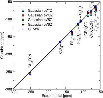
Figure 1: (Color online) Experimental vs. calculated ¹⁹F chemical shifts in ppm, with respect to CF₃Cl. For sake of clarity the chemical shift of F₂ is not shown.

IV.3 Solids

In this section we present the ²⁹Si and ¹⁷O chemical shifts calculated by our converse method in four SiO₂ polymorphs: quartz, $\beta$-cristobalite, coesite and stishovite. Coesite and stishovite are metastable phases that form at high temperature and pressures developed during a meteor impact. NASA Besides their natural occurrence in meteors, they can also be artificially synthesized by shock experiments.

We adopted the experimental crystal structures and atom positions in all calculations. We used a cutoff of 100 Ryd and a k-point mesh of 8$\times$8$\times$8 for quartz, $\beta$-cristobalite and stishovite. In the case of coesite, having the largest primitve cell (48 atoms), we used a k-point mesh of 4$\times$4$\times$4. In Table 6 we show a comparison between the calculated and the experimental chemical shifts for the four crystals. We determined the ²⁹Si and ¹⁷O reference shielding as the intercept of the least-square linear interpolation of the $(\sigma_{\mathrm{calc}},\delta_{\mathrm{expt}})$ pairs. Note that the nuclear magnetic dipole ${\bf m}_{s}$ breaks the symmetry of the hamiltonian. Thus, we retained only the symmetry operations that map site $s$ in $s^{\prime}$ without changing the orientation of the magnetic dipole (i.e. $s\rightarrow s^{\prime},{\bf m}_{s}={\bf m}_{s^{\prime}}$).

Another important point is that in periodic systems we are not just including one nuclear dipole, but rather an infinite array. Thus, interactions between ${\bf m}_{s}$ and its infinite periodic replicas become important, and the chemical shift should be converged with respect to the supercell size. To test for this convergence, we repeated the calculations for quartz and $\beta$-cristobalite in a larger supercell and we found a change in chemical shift of less than 0.1 ppm. This rapid convergence is due to the $1/r^{3}$ decay of the magnetic dipole interactions.

Table 6: Calculated and experimental ²⁹Si and ¹⁷O NMR chemical shifts of four SiO₂ crystals in ppm. Experimental data was taken from Refs. [NASA, ] and [profeta03, ]. In the case of coesite all inequivalent chemical shifts are reported.

Mineral	Calc. $\delta$ [ppm]	Expt. $\delta$ [ppm]
	29Si
quartz	$-$107.10	$-$107.73
$\beta$-cristobalite	$-$108.78	$-$108.50
stishovite	$-$184.13	$-$191.33
coesite	$-$107.30	$-$107.73
	$-$113.35	$-$114.33
	17O
quartz	43.52	40.8
$\beta$-cristobalite	40.35	37.2
stishovite	116.35	N/A
coesite	26.35	29
	39.66	41
	52.70	53
	56.84	57
	59.03	58

IV.4 Large Systems

Reactive sites in biological systems such as organometallic molecules, as well as inorganic materials, are of great importance. In particular, there is a surge of interest in studying copper(I) reactive sites using solid-state NMR. NMR experiments on these materials are challenging because of the large nuclear quadrupole moments of ⁶³Cu and ⁶⁵Cu. Here, we present the results for the copper-phosphine metallocene, tetramethylcyclopentadienyl copper(I) triphenylphosphine (CpCuPPh3), which as a solid contains 228 atoms in a primitive orthorhombic unit cell. The molecular structure is shown in Fig. 2. The properties of the shielding tensor for the copper environment were observed experimentally for the solid material, and simulated using quantum-chemical methods on the molecular complex. tang07

While the converse approach can calculate the chemical shift for this large system easily, it is more challenging for the linear-response method, which in our experience took much longer in general, did not finish at all, or was unable to handle such large systems. We calculated the copper chemical shift for CpCuPPh3 using the converse method with an energy cutoff of 80 Ry in the self-consistent step and PBE pseudopotentials. While previous quantum-chemical calculations were able to reasonably reproduce the experimental span (1300 ppm) and the skew (0.95) of the chemical shielding tensor, they were not able to calculate the chemical shift itself (0 ppm relative to copper (I) chloride), with an inaccuracy of several hundred ppm. tang07 In addition to yielding excellent agreement with experiment to within 2 ppm for the chemical shift, our calculations also gave good results for the span (1038 ppm) and the skew (0.82) of the chemical shielding tensor.

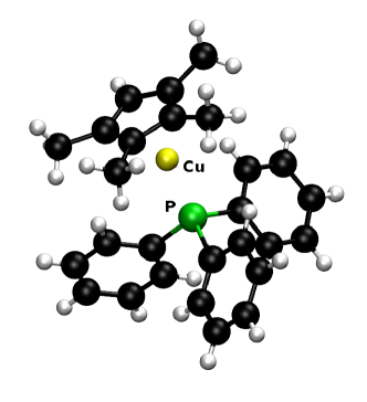
Figure 2: (Color online) The molecular structure of the metallocene, tetramethylcyclopentadienyl copper(I) triphenylphosphine (CpCuPPh3). The copper is shown in gold (light gray) forming the metallocene bond, while the phosphorus is green (gray). The crystal structure of this materials consists of a 228-atom orthorhombic unit cell.

V Discussion

The results presented in the previous sections and in a previous work Thonhauser_09 show that DFT is able to predict accurately the chemical shift of molecules and solids. In general, we expect this to be true for any weakly-correlated system, well described by the generalized-gradient approximation (GGA). In addition to that, relativistic corrections to the NMR chemical shifts are negligible for all light elements in the periodic table, and become important starting from 4th row elements.

However, there will always exist “difficult” cases in which relativistic corrections cannot be neglected and/or one has to go beyond DFT with standard local functionals. This is an active field of research in quantum chemistry NMR-dirac ; NMR-beyond-DFT and today it is customary to compute NMR chemical shifts with semi-local hybrid DFT functionals (such as B3LYP). Most quantum-chemistry codes allow the inclusion of relativistic effects (spin orbit) by perturbation theory; furthermore, fully-relativistic (four component) solutions of the Dirac-Breit equation have recently been implemented. NMR-dirac

To the best of our knowledge, all existing ab-initio codes, calculate NMR shifts by perturbation theory. Among them, localized-basis sets are the most popular choice to expand wave functions. This leads to very complicated mathematical expressions and to gauge-dependent results. Only two plane-wave, linear-response implementations Pickard_Mauri_01 ; Sebastiani_01 have been reported. Our converse-NMR method is built on Mauri’s GIPAW method, but has the advantage of circumventing the need for a linear response framework.

The main advantage of our converse-NMR method is that it requires only the ground state wave functions and Hamiltonian to calculate the orbital magnetization. Since no external magnetic field is included in the calculation, our method solves the gauge-origin problem. Moreover, “difficult cases” can be treated easily by our converse method, provided that relativistic corrections and many-body effects are included in the Hamiltonian. Thus, one can concentrate effectively all efforts in developing advanced post-DFT theories (i.e. DFT+U, DMFT, hybrid functionals, self-interaction-free methods) and benchmark them against NMR experiments.

VI Summary

In this paper we have generalized the recently developed converse NMR approach Thonhauser_09 such that it can be used in conjunction with norm-conserving, non-local pseudopotentials. We have tested our approach both in finite and periodic systems, on small molecules, four silicate minerals and a molecular crystal. In all cases, we have found very good agreement with established methods and experimental results.

The main advantage of the converse-NMR method is that it requires only the ground state wave functions and Hamiltonian, circumventing the need of any linear response treatment. This is of paramount importance for the rapid development and validation of new methods that go beyond DFT.

Currently, we are applying the converse NMR method to study large biological systems such as nuclei acidsCooper_08 and drug-DNA interactionsCooper2_08 ; Li_09 in conjunction with a recently developed van der Waals exchange-correlation functional.Thonhauser_07 ; Langreth_09 We are also exploring the possibility to calculate non-perturbatively the Knight shift in metals. Finally, the converse method can be used to calculate the EPR g-tensor in molecules and solids. ceresoli-EPR

VII Acknowledgments

This work was supported by the DOE/SciDAC Institute on Quantum Simulation of Materials and Nanostructures. All computations were performed on the Wake Forest University DEAC Cluster with support from the Wake Forest University Science Research Fund. D. C. acknowledges partial support from ENI.

Appendix A The GIPAW transformation

The starting point is the projector augmented wave (PAW) transformation: Blochl_94

$$\mathcal{T}=1+\sum_{{\bf R},n}\left(\ket{\phi_{{\bf R},n}}-\ket{\widetilde{\phi}_{{\bf R},n}}\right)\bra{\widetilde{p}_{{\bf R},n}}$$ (30)

which connects an all-electron wave function $\ket{\psi}$ to the corresponding pseudopotential wave function $\ket{\widetilde{\psi}}$ via: $\ket{\psi}=\mathcal{T}\ket{\widetilde{\psi}}$. Here, $\ket{\phi_{{\bf R},n}}$ are all-electron partial waves, $\ket{\widetilde{\phi}_{{\bf R},n}}$ are pseudopotential partial waves, and $\bra{\widetilde{p}_{{\bf R},n}}$ are PAW projectors. The sum runs over the atom positions ${\bf R}$. $n$ is a combined index that runs over the set of projectors attached to atom ${\bf R}$. In the original PAW formalism, there are two sets of projectors per angular momentum channel ($0,\dots,l_{\mathrm{max}}$), each with $(2l+1)$ projectors for a total of $2(l_{\mathrm{max}}+1)^{2}$ PAW projectors.

The expectation value of an all-electron operator $O_{\mathrm{AE}}$ between all-electron wave functions can then be expressed as the expectation value of a pseudo operator $O_{\mathrm{PS}}$ between pseudo wave functions as $\braket{\psi}{O_{\mathrm{AE}}}{\psi}=\braket{\widetilde{\psi}}{O_{\mathrm{PS}}}{\widetilde{\psi}}$, where the $O_{\mathrm{PS}}$ is given by:

$$O_{\mathrm{PS}}\equiv\mathcal{T}^{+}O_{\mathrm{AE}}\mathcal{T}=\\ =O_{\mathrm{AE}}+\sum_{{\bf R},nm}\ket{\widetilde{p}_{{\bf R},n}}\Big{[}\braket{\phi_{{\bf R},n}}{O_{\mathrm{AE}}}{\phi_{{\bf R},m}}-\\ -\braket{\widetilde{\phi}_{{\bf R},n}}{O_{\mathrm{AE}}}{\widetilde{\phi}_{{\bf R},m}}\Big{]}\bra{\widetilde{p}_{{\bf R},m}}$$ (31)

In the presence of external magnetic fields the PAW transformation is no longer invariant with respect to translations (except in the very simple case of only one augmentation region). This deficiency was resolved by Mauri et al. who developed the GIPAW (“gauge including PAW”) method Pickard_Mauri_01 , which is similar to the PAW transformation from Eq. (31) but with the inclusion of phase factor compensating the gauge term arising from the translation of a wave function in a magnetic field. The GIPAW transformation in the symmetric gauge reads:

$$\mathcal{T}_{G}=1+\sum_{{\bf R},n}e^{(i/2c){\bf r}\cdot{\bf R}\times{\bf B}}\left(\ket{\phi_{{\bf R},n}}-\ket{\widetilde{\phi}_{{\bf R},n}}\right)\cdot\\ \bra{\widetilde{p}_{{\bf R},n}}e^{-(i/2c){\bf r}\cdot{\bf R}\times{\bf B}}$$ (32)

and the corresponding pseudopotential operator $O_{\mathrm{PS}}$ is:

$$O_{\mathrm{PS}}\equiv{\mathcal{T}_{G}}^{+}O_{\mathrm{AE}}\mathcal{T}_{G}=O_{\mathrm{AE}}+\sum_{{\bf R},nm}e^{(i/2c){\bf r}\cdot{\bf R}\times{\bf B}}\ket{\widetilde{p}_{{\bf R},n}}\cdot\\ \Big{[}\braket{\phi_{{\bf R},n}}{e^{-(i/2c){\bf r}\cdot{\bf R}\times{\bf B}}\,O_{\mathrm{AE}}\,e^{(i/2c){\bf r}\cdot{\bf R}\times{\bf B}}}{\phi_{{\bf R},m}}-\\ -\braket{\widetilde{\phi}_{{\bf R},n}}{e^{-(i/2c){\bf r}\cdot{\bf R}\times{\bf B}}\,O_{\mathrm{AE}}\,e^{(i/2c){\bf r}\cdot{\bf R}\times{\bf B}}}{\widetilde{\phi}_{{\bf R},m}}\Big{]}\\ \cdot\bra{\widetilde{p}_{{\bf R},m}}e^{-(i/2c){\bf r}\cdot{\bf R}\times{\bf B}}$$ (33)

In the following we will refer to the often occurring part $\hat{O}_{\mathrm{AE}}=e^{-(i/2c){\bf r}\cdot{\bf R}\times{\bf B}}\,O_{\mathrm{AE}}\,e^{(i/2c){\bf r}\cdot{\bf R}\times{\bf B}}$ as inner operator and denote it with a hat. The above expression allows us to calculate accurate expectation values of operators within a pseudopotential approach. In this work we carry out the derivation working in the symmetric gauge ${\bf A}({\bf r})=(1/2){\bf B}\times{\bf r}$. This is not an issue, since all physical quantities we are working with, are gauge invariant.

One useful property of the GIPAW transformation is:

$$e^{-(i/2c){\bf r}\cdot{\bf R}\times{\bf B}}\Big{[}{\bf p}+\frac{1}{c}{\bf A}({\bf r})\Big{]}^{n}e^{(i/2c){\bf r}\cdot{\bf R}\times{\bf B}}=\\ =\Big{[}{\bf p}+\frac{1}{c}{\bf A}({\bf r}-{\bf R})\Big{]}^{n}$$ (34)

Appendix B Periodic systems

Note that the set of equations (II.2) are well defined also in periodic boundary conditions. In fact, ${\bf M}_{\mathrm{bare}}$ can be calculated by the Modern Theory of the Orbital Magnetization Resta_05 ; Thonhauser_06 ; Ceresoli_06 ; Niu as:

$${\bf M}_{\mathrm{bare}}=-\frac{1}{2c}\mathrm{Im}\sum_{n{\bf k}}f(\epsilon_{n{\bf k}})\bra{\partial_{\bf k}u_{n{\bf k}}}\\ \times\left(\mathcal{H}_{\bf k}+\epsilon_{n{\bf k}}-2\epsilon_{\mathrm{F}}\right)\ket{\partial_{\bf k}u_{n{\bf k}}}\Big{|}_{\mathrm{GIPAW}}$$ (35)

where $\mathcal{H}_{\bf k}$ is the GIPAW hamiltonian, $\epsilon_{n{\bf k}}$ and $\ket{u_{n{\bf k}}}$ are its eigenvalues and eigenvectors.

The position operator appearing in the other terms in Eq. (II.2) is well defined because the projectors $\ket{\beta_{{\bf R},n}}$ and $\ket{\widetilde{p}_{{\bf R},n}}$ are non-vanishing only inside an augmentation sphere, centered around atom ${\bf R}$.

The expression of ${\bf M}_{\mathrm{NL}},{\bf M}_{\mathrm{para}}$ and ${\bf M}_{\mathrm{para}}$ can be further manipulated in order to work with Bloch wave functions. In the following part, we show it only for ${\bf M}_{\mathrm{NL}}$, since ${\bf M}_{\mathrm{para}}$ is similar. The term ${\bf M}_{\mathrm{dia}}$ can be manipulated instead in a trivial way.

Let’s consider the expectation value of

$$({\bf r}-{\bf R})\times\left[{\bf r}-{\bf R},V_{\bf R}^{\mathrm{NL}}\right]=-({\bf r}-{\bf R})\times\left(V_{\bf R}^{\mathrm{NL}}\right)\,({\bf r}-{\bf R})$$ (36)

on a Bloch state $\ket{\psi_{n{\bf k}}}=e^{i{\bf k}{\bf r}}\ket{u_{n{\bf k}}}$:

$$-\sum_{\bf R}\braket{u_{n{\bf k}}}{e^{-i{\bf k}{\bf r}}({\bf r}-{\bf R})\times(V_{\bf R}^{\mathrm{NL}})\,({\bf r}-{\bf R})e^{i{\bf k}{\bf r}}}{u_{n{\bf k}}}=$$ (37)

$$=-\sum_{{\bf L}\bm{\tau}}\sum_{ij}\braket{u_{n{\bf k}}}{e^{-i{\bf k}{\bf r}}({\bf r}-{\bf L}-\bm{\tau})\ket{\beta_{{\bf L}+\bm{\tau},i}}\times v^{L+\tau}_{ij}\bra{p_{{\bf L}+\bm{\tau},j}}({\bf r}-{\bf L}-\bm{\tau})e^{i{\bf k}{\bf r}}}{u_{n{\bf k}}}\;,$$ (38)

where ${\bf L}$ are the real space lattice vectors (not to be confused with the angular momentum operator) and $\bm{\tau}$ are the position of the atoms in the unit cell. Inserting two canceling phase factors:

$$\cdots=-\sum_{{\bf L}\tau}\sum_{ij}\braket{u_{n{\bf k}}}{e^{-i{\bf k}({\bf r}-{\bf L}-\bm{\tau})}({\bf r}-{\bf L}-\bm{\tau})\ket{\beta_{{\bf L}+\bm{\tau},i}}\times v^{L+\tau}_{ij}\bra{\beta_{{\bf L}+\bm{\tau},j}}({\bf r}-{\bf L}-\bm{\tau})e^{i{\bf k}({\bf r}-{\bf L}-\bm{\tau})}}{u_{n{\bf k}}}$$ (39)

one can recognize immediately the ${\bf k}$ derivative of the KB projectors. In addition, since the KB projectors vanish outside their augmentation regions, it is possible to insert a second sum over ${\bf L}^{\prime}$ running on the right hand side of the cross product:

$$\cdots=-\sum_{{\bf L}{\bf L}^{\prime}\tau}\sum_{ij}\braket{u_{n{\bf k}}}{(-1/i)\partial_{\bf k}\left(e^{-i{\bf k}({\bf r}-{\bf L}-\bm{\tau})}\ket{\beta_{{\bf L}+\bm{\tau},i}}\right)\times v^{L+\tau}_{ij}\,(1/i)\partial_{\bf k}\left(\bra{\beta_{{\bf L}^{\prime}+\bm{\tau},j}}e^{i{\bf k}({\bf r}-{\bf L}-\bm{\tau})}\right)}{u_{n{\bf k}}}$$ (40)

$$=-\sum_{\tau}\sum_{ij}\braket{u_{n{\bf k}}}{\partial_{\bf k}\left(\sum_{\bf L}e^{-i{\bf k}({\bf r}-{\bf L}-\bm{\tau})}\ket{\beta_{{\bf L}+\bm{\tau},i}}\right)\times v^{L+\tau}_{ij}\,\partial_{\bf k}\left(\sum_{{\bf L}^{\prime}}\bra{\beta_{{\bf L}^{\prime}+\bm{\tau},j}}e^{i{\bf k}({\bf r}-{\bf L}^{\prime}-\bm{\tau})}\right)}{u_{n{\bf k}}}$$ (41)

In periodic systems the structure factors can be absorbed by the projectors:

$$V_{\mathrm{NL}}^{\bf k} = \sum_{\bm{\tau}}\sum_{ij}\ket{\beta_{\bm{\tau},i}^{\bf k}}v_{\tau,ij}\bra{\beta_{\bm{\tau},j}^{\bf k}}$$ (42)

$$\ket{\beta_{\bm{\tau},i}^{\bf k}} = \sum_{\bf L}e^{-i{\bf k}({\bf r}-{\bf L}-\bm{\tau})}\ket{\beta_{{\bf L}+\bm{\tau},i}}$$ (43)

Finally:

$${\bf M}_{\mathrm{NL}} = \frac{1}{2c}\sum_{n{\bf k}}^{\mathrm{occ}}\sum_{\bm{\tau},ij}\frac{1}{i}\Braket{u_{n{\bf k}}}{\partial_{\bf k}\beta_{\bm{\tau},i}^{\bf k}}\times v_{\tau,ij}\,\Braket{\partial_{\bf k}\beta_{\tau,j}^{\bf k}}{u_{n{\bf k}}}$$ (44a)

$${\bf M}_{\mathrm{para}} = \frac{1}{2c}\sum_{n{\bf k}}^{\mathrm{occ}}\sum_{\bm{\tau},ij}\frac{1}{i}\Braket{u_{n{\bf k}}}{\partial_{\bf k}\widetilde{p}_{\bm{\tau},i}^{\bf k}}\times k_{\tau,ij}\,\Braket{\partial_{\bf k}\widetilde{p}_{\tau,j}^{\bf k}}{u_{n{\bf k}}}$$ (44b)

$${\bf M}_{\mathrm{dia}} = -\frac{1}{2c}\sum_{n{\bf k}}^{\mathrm{occ}}\Braket{u_{n{\bf k}}}{\widetilde{p}_{\bm{\tau},i}^{\bf k}}\bm{e}_{\tau,ij}\,\Braket{\widetilde{p}_{\tau,j}^{\bf k}}{u_{n{\bf k}}}$$ (44c)

This completes the main result and it allows us to calculate the orbital magnetization in the presence of non-local pseudopotentials. With this result we can now easily and efficiently calculate the NMR chemical shift for elements heavier then hydrogen using Eq. (1).

References

- (1) I. I. Rabi, J. R. Zacharias, S. Millman, and P. Kusch, Phys. Rev. 53, 318 (1938).
- (2) Encyclopedia of NMR, edited by D.M. Grant and R.K. Harris (Wiley, London, 1996).
- (3) W. Kutzelnigg, U. Fleischer, and M. Schindler, NMR Basic Principles and Progress (Springer, Berlin, 1990).
- (4) F. Mauri, B. G. Pfrommer, and S. G. Louie, Phys. Rev. Lett. 77, 5300 (1996).
- (5) D. Sebastiani and M. Parrinello, J. Phys. Chem. A 105, 1951 (2001).
- (6) C. J. Pickard and F. Mauri, Phys. Rev. B 63, 245101 (2001).
- (7) C. J. Pickard and F. Mauri, Phys. Rev. Lett. 91, 196401 (2003).
- (8) J. R. Yates, C. J. Pickard, and F. Mauri, Phys. Rev. B 76, 024401 (2007).
- (9) T. Thonhauser, D. Ceresoli, A. Mostofi, N. Marzari, R. Resta, and D. Vanderbilt, J. Chem. Phys. 131, 101101 (2009).
- (10) T. Thonhauser, D. Ceresoli, and N. Marzari, Int. J. Quantum Chem. 109, 3336 (2009).
- (11) L. Kleinman and D. M. Bylander, Phys. Rev. Lett. 48, 1425 (1982).
- (12) J. D. Jackson, Classical Electrodynamics, 2nd ed. (Wiley, New York, 1975).
- (13) S. Sharma, S. Pittalis, S. Kurth, S. Shallcross, J. K. Dewhurst and E. K. U. Gross, Phys. Rev. B 76, 100401 (2007).
- (14) R. Resta, D. Ceresoli, T. Thonhauser, and D. Vanderbilt, Chem. Phys. Chem. 6, 1815 (2005).
- (15) T. Thonhauser, D. Ceresoli, D. Vanderbilt, and R. Resta, Phys. Rev. Lett. 95, 137205 (2005).
- (16) D. Ceresoli, T. Thonhauser, D. Vanderbilt, and R. Resta, Phys. Rev. B 74, 024408 (2006).
- (17) Di Xiao, J. Shi, and Q. Niu, Phys. Rev. Lett. 95, 137204 (2005); J. Shi, G. Vignale, Di Xiao, and Qian Niu, Phys. Rev. Lett. 99, 197202 (2007).
- (18) N. Sai, K. M. Rabe, and D. Vanderbilt, Phys. Rev. B 66, 104108 (2002).
- (19) C. J. Pickard and M. C. Payne, Phys. Rev. B 62, 4383 (2000); M. Iannuzzi and M. Parrinello, Phys. Rev. B 64, 233104 (2001).
- (20) P. Giannozzi, S. Baroni, N. Bonini, M. Calandra, R. Car, C. Cavazzoni, D. Ceresoli, G. L. Chiarotti, M. Cococcioni, I. Dabo, A. Dal Corso, S. de Gironcoli, S. Fabris, G. Fratesi, R. Gebauer, U. Gertsmann, C. Gougoussis, A. Kokalj, M. Lazzeri, L. Martin-Samos, N. Marzari, F. Mauri, R. Mazzarello, S. Paolini, A. Pasquarello, L. Paulatto, C. Sbraccia, S. Scandolo, G. Sclauzero, A. P. Seitsonen, A. Smogunov, P. Umari and R. M. Wentzcovitch, J. Phys.: Condens. Matter 21, 395502 (2009); http://www.quantum-espresso.org
- (21) N. Troullier, J. L. Martins, Phys. Rev. B 43, 1993 (1991).
- (22) J. P. Perdew, K. Burke, and M. Ernzerhof, Phys. Rev. Lett. 78, 1396 (1997).
- (23) D. Maisch, P. Wadhwani, S. Afonin, C. Böttcher, B. Koksch, and A. S. Ulrich, J. Am. Chem. Soc. 131, 15596 (2009).
- (24) Gaussian 03, Revision D.01, M. J. Frisch, G. W. Trucks, H. B. Schlegel, G. E. Scuseria, M. A. Robb, J. R. Cheeseman, J. A. Montgomery, Jr., T. Vreven, K. N. Kudin, J. C. Burant, J. M. Millam, S. S. Iyengar, J. Tomasi, V. Barone, B. Mennucci, M. Cossi, G. Scalmani, N. Rega, G. A. Petersson, H. Nakatsuji, M. Hada, M. Ehara, K. Toyota, R. Fukuda, J. Hasegawa, M. Ishida, T. Nakajima, Y. Honda, O. Kitao, H. Nakai, M. Klene, X. Li, J. E. Knox, H. P. Hratchian, J. B. Cross, V. Bakken, C. Adamo, J. Jaramillo, R. Gomperts, R. E. Stratmann, O. Yazyev, A. J. Austin, R. Cammi, C. Pomelli, J. W. Ochterski, P. Y. Ayala, K. Morokuma, G. A. Voth, P. Salvador, J. J. Dannenberg, V. G. Zakrzewski, S. Dapprich, A. D. Daniels, M. C. Strain, O. Farkas, D. K. Malick, A. D. Rabuck, K. Raghavachari, J. B. Foresman, J. V. Ortiz, Q. Cui, A. G. Baboul, S. Clifford, J. Cioslowski, B. B. Stefanov, G. Liu, A. Liashenko, P. Piskorz, I. Komaromi, R. L. Martin, D. J. Fox, T. Keith, M. A. Al-Laham, C. Y. Peng, A. Nanayakkara, M. Challacombe, P. M. W. Gill, B. Johnson, W. Chen, M. W. Wong, C. Gonzalez, and J. A. Pople, Gaussian, Inc., Wallingford CT, 2004.
- (25) Basis set exchange, https://bse.pnl.gov/bse/portal
-
(26)
19F Reference standards, document available at:
http://chemnmr.colorado.edu/manuals/19F_NMR_Reference_Standards.pdf - (27) J. Nehring and A. Saupe, J. Chem. Phys. 52, 1307 (1970).
- (28) M. B. Boslough, R. T. Cygan, R. T. and J. R. Kirkpatrick, Abstracts of the 24th Lunar and Planetary Science Conference, held in Houston, TX, 15-19 March 1993, p. 149 (1993).
- (29) M. Profeta, F. Mauri and C. J. Pickard, J. Am. Chem. Soc. 125, 541 (2003).
- (30) J. A. Tang, B. D. Ellis, T. H. Warren, J. V. Hanna, C. L. B. Macdonald, and R. W. Schurko, J. Am. Chem. Soc. 129, 13049-13065, (2007).
- (31) M. Iliaš, T. Saue, T. Enevoldsen and H. J. Aa. Jensen, J. Chem. Phys. 131, 124110 (2009).
- (32) A. Soncini, A. M. Teale, T. Helgaker, F. De Proft and D. J. Tozer, J. Chem. Phys. 129, 074101 (2008).
- (33) V. R. Cooper, T. Thonhauser, and D. C. Langreth, J. Chem. Phys. 128, 204102 (2008).
- (34) V. R. Cooper, T. Thonhauser, A. Puzder, E. Schröder, B. I. Lundqvist, and D. C. Langreth, J. Am. Chem. Soc. 130, 1304 (2008).
- (35) S. Li, V. R. Cooper, T. Thonhauser, B. I. Lundqvist, and D. C. Langreth, J. Phys. Chem. B 113, 11166 (2009).
- (36) T. Thonhauser, V. R. Cooper, S. Li, A. Puzder, P. Hyldgaard, and D. C. Langreth, Phys. Rev. B 76, 125112 (2007).
- (37) D. C. Langreth, B. I. Lundqvist, S.D. Chakarova-K\a”ck, V. R. Cooper, M. Dion, P. Hyldgaard, A. Kelkkanen, J. Kleis, L. Kong, S. Li, P. G. Moses, E. Murray, A. Puzder, H. Rydberg, E. Schröder, and T. Thonhauser, J. Phys.: Condens. Matter 21, 084203 (2009).
- (38) D. Ceresoli, U. Gerstmann, A. P. Seitsonen and F. Mauri, Phys. Rev. B 81, 060409 (2010).
- (39) P. E. Blöchl, Phys. Rev. B 50, 17953 (1994).