SPIDER – III. Environmental Dependence of the Fundamental Plane of Early-type Galaxies

Abstract

We analyse the Fundamental Plane (FP) relation of $39,993$ early-type galaxies (ETGs) in the optical (griz) and $5,080$ ETGs in the Near-Infrared (YJHK) wavebands, forming an optical$+$NIR sample of $4,589$ galaxies. We focus on the analysis of the FP as a function of the environment where galaxies reside. We characterise the environment using the largest group catalogue, based on 3D data, generated from SDSS at low redshift ($z<0.1$). We find that the intercept $``c^{\prime\prime}$ of the FP decreases smoothly from high to low density regions, implying that galaxies at low density have on average lower mass-to-light ratios than their high-density counterparts. The $``c^{\prime\prime}$ also decreases as a function of the mean characteristic mass of the parent galaxy group. However, this trend is weak and completely accounted for by the variation of $``c^{\prime\prime}$ with local density. The variation of the FP offset is the same in all wavebands, implying that ETGs at low density have younger luminosity-weighted ages than cluster galaxies, consistent with the expectations of semi-analytical models of galaxy formation. We measure an age variation of $\sim 0.048$ dex ($\sim 11\%$) per decade of local galaxy density. This implies an age difference of about $32\%$ ($\sim 3\,Gyr$) between galaxies in the regions of highest density and the field. We find the metallicity decreasing, at $\sim 2$ $\sigma$, from low to high density. We also find $2.5\,\sigma$ evidence that the variation in age per decade of local density augments, up to a factor of two, for galaxies residing in massive relative to poor groups. The velocity dispersion slope of the FP, $``a^{\prime\prime}$, tends to decrease with local galaxy density, with galaxies in groups having smaller $``a^{\prime\prime}$ than those in the field, independent of the waveband used to measure the structural parameters. Environmental effects (such as tidal stripping) may elucidate this result, producing a steeper variation of dark-matter fraction and/or non-homology along the ETG’s sequence at higher density. In the optical, the surface brightness slope, $``b^{\prime\prime}$, of the FP increases with local galaxy density, being larger for group relative to field galaxies. The difference vanishes in the NIR, as field galaxies show a small ($\sim 2.5\%$), but significant increase of $``b^{\prime\prime}$ from $g$ through $K$, while group galaxies (particularly those in rich clusters) do not. The trend of $``b^{\prime\prime}$ with the environment results from galaxies residing in more massive clusters, since for groups no variation of $``b^{\prime\prime}$ with local density is detected. A possible explanation for these findings is that the variation of stellar population properties with mass in ETGs is shallower for galaxies at high density, resulting from tidal stripping and quenching of star formation in galaxies falling into the group’s potential well. We do not detect any dependence of the FP coefficients on the presence of substructures in parent galaxy groups.

1 Introduction

A robust prediction of hierarchical theories of galaxy formation is that the environment plays an important role in shaping the galaxian properties. From the observational viewpoint, this is successfully confirmed by the existence, for instance, of the well established morphology-density relation (Dressler, 1980), for which denser environments are preferably populated by galaxies with early-type morphology in contrast to the late-type dominated field regions.

The role of environment in shaping the properties of ETGs – the most massive galaxies in the local Universe – is still an open question in our understanding of galaxy formation and evolution. Studies of the colour–magnitude (hereafter CM) relation in the low-redshift-Universe have found no significant difference in the average colour of ETGs among high- and low-density environments, implying either a tiny difference or a strong anti-correlated variation of stellar population properties, i.e. age and metallicity, with environment (Bernardi et al., 2003b; Hogg et al., 2004; Haines et al., 2006). Even small differences in the star formation history of galaxies residing in different environments would be magnified as one approaches the galaxy formation epoch. Several studies have found no remarkable difference in the properties of cluster and field galaxies at high redshift. For instance, Koo et al. (2005a, b) found that both field and cluster ETGs have very similar CM relations at redshift $z\sim 0.8$. Cool et al. (2006) also reported that the offset and slope of the CM relation of field and cluster galaxies are fully consistent up to redshift $z\sim 0.4$. Pannella et al. (2009) found that ETGs have similar characteristic ages, independent of the environment they belong to. An opposite picture comes out of spectroscopic studies of ETGs at redshift $z\sim 0$. Many authors have reported younger luminosity-weighted ages for field relative to cluster galaxies, with the age difference amounting to $\sim 1$–$2$ Gyr (e.g. Guzman et al. 1992; Trager et al. 2000; Kuntschner et al. 2002; Terlevich & Forbes 2002; Thomas et al. 2005; Bernardi et al. 2006; Clemens et al. 2009). Such difference seems to exist also when considering galaxies residing in high-density, low-velocity dispersion systems, such as the Hickson Compact Groups (de La Rosa et al., 2007).

A even more puzzling issue is the difference in metal content of ETGs among different environments, as different studies have found that field ETGs are more metal-rich (Thomas et al., 2005; de La Rosa et al., 2007; Kuntschner et al., 2002; Clemens et al., 2009), as metal-rich as (Bernardi et al., 2006; Annibali et al., 2007), or even more metal-poor than their cluster counterparts (Gallazzi et al., 2006). A main feature of the spectroscopic investigations is that the galaxy spectra, and hence the inferred stellar population properties, refer to the galaxy inner region, typically inside one effective radius. On the other hand, ETGs are know to possess internal colour gradients, with their central part being redder than the outskirts (see Wu et al. 2005; Roche, Bernardi, & Hyde 2009; and references therein). These gradients are mainly due to metallicity (Peletier et al., 1990), with a small, but significant contribution from age (La Barbera & de Carvalho, 2009; Clemens et al., 2009). Moreover, as shown by La Barbera et al. (2005), colour gradients seem to depend on the environment where galaxies reside, hence complicating the environmental comparison of spectroscopic properties.

Due to its small intrinsic dispersion (see e.g. Gargiulo et al. 2009; Hyde & Bernardi 2009; and references therein), the Fundamental Plane (FP) relation of ETGs (Dressler et al., 1987; Djorgovski & Davis, 1987), i.e. the scaling law involving radius, velocity dispersion, and surface brightness, is a powerful tool to measure their mass-to-light ratio (see e.g. van Dokkum & Franx 1996). This results from interpreting the FP as a consequence of mass-to-light ratio systematically varying with mass and the non-homology of ETGs (see e.g. Hjorth & Madsen 1995; Capelato, de Carvalho, & Carlberg 1995; Ciotti & Lanzoni 1997; Graham & Colless 1997; Busarello et al. 1997; Trujillo, Burkert, & Bell 2004; Bolton et al. 2007; Tortora et al. 2009). Several studies have used the FP to constrain the environmental variation, at a given mass, of galaxy luminosity. Even in this case, a contradictory picture emerges.  Bernardi et al. (2006) found the FP relation at low- and high-density to have consistent slopes but a significant offset, interpreting it as a difference of $\sim 1$ Gyr in the formation epoch of field and cluster ETGs. On the contrary, D’Onofrio et al. (2008), analysing galaxies in massive nearby clusters, found also significant variations of the slopes with local density. High redshift studies of the FP have reported a consistent evolution of the mass-to-light ratio of ETGs among different environments, implying the same formation epoch of field and cluster galaxies   (Jørgensen et al., 2006; van Dokkum & van der Marel, 2006). van der Wel et al. (2005) also found that the difference in mass-to-light ratios between field and cluster galaxies depends on galaxy mass, with low mass systems exhibiting a strong differential evolution (see also Pahre, Djorgovski, & de Carvalho 2001; di Serego Alighieri et al. 2006).

This work is the third paper of a series aimed to investigate the properties of bright ($M_{r}<-20$) ETGs as a function of the environment where they reside, in the low-redshift-Universe ($0.05<z<0.1$). The Spheroid’s Panchromatic Investigation in Different Environmental Regions (SPIDER; see La Barbera et al. 2010a, hereafter paper I) is based on a sample of 39,993 ETGs with photometry and spectroscopy available from SDSS, and Near-Infrared (NIR) photometry available from the UKIDSS-Large Area Survey (LAS;  Lawrence et al. 2007). Here, we define the environment where the ETGs reside, and investigate the environmental dependence of the FP. To this effect, we cross-correlate the SPIDER sample to the largest group catalogue, based on 3D data, generated from SDSS at low redshift ($z<0.1$). This group catalogue contains 10,124 systems selected using a redshift-space friends-of-friends (FoF) algorithm from the SDSS data release 7 (DR7, covering 9,380 square degrees of the northern sky). Notice that we chose not to cross-correlate the SPIDER sample with existing SDSS-based group catalogues, as they do not cover either the entire area or the (low-)redshift range of the SPIDER survey. For instance, the maxBCG catalogue is a volume limited cluster sample spanning the reshift range $0.10<z<0.30$ (Koester et al., 2007), while the SPIDER sample is at $z<0.1$. The C4 catalogue (Miller et al., 2005) spans the redshift range of $0.02$ to $0.17$, but it covers only $2,600$ square degrees on the sky, being based on SDSS-DR2. The FoF group/cluster catalogue we use in the present study has the main advantage of providing a complete sample of groups and clusters in the local Universe, covering the large sky area of SDSS-DR7. This allows us to derive the FP relation in a wide range of environments using both optical and NIR data, and characterising the environments in terms of both $``local^{\prime\prime}$ (e.g. galaxy density) and $``global^{\prime\prime}$ (e.g. parent group mass) observables. The large sample size provided by the SDSS+UKIDSS data allows us not only to analyse the offset but also the slopes of the FP as a function of environment.

The layout of the paper is the following. In Sec. 2, we describe the samples of ETGs. Sec. 3 presents the catalogue of galaxy groups we use to define the environment, while Sec. 4 describes the properties measured for each group, that define the $``global^{\prime\prime}$ environment of ETGs. Sec. 5 deals with the measurement of quantities, such as local galaxy density, that define the $``local^{\prime\prime}$ environment. Sec. 6 introduces the FP relation, and the way we measure its slopes and intercept. In Sec. 7 we derive the intercept of the FP in different wavebands as a function of environment. Sec. 8 analyses how the offset of the FP constrains the difference in stellar population content, i.e. age and metallicity, of ETGs among different environments. Sec. 9 describes the dependence of the slopes of the FP on local and global environment. In Sec. 10, we discuss the main results of this work. A summary is provided in Sec. 11. Throughout the paper, we adopt a cosmology with $\Omega_{\rm m}=$ 0.3, $\Omega_{\lambda}=$ 0.7, and H${}_{0}=75$ $\rm km$ $s^{-1}$ Mpc^-1.

2 Samples of ETGs

The SPIDER sample consists of $39,993$ ETGs, with available $griz$ photometry and spectroscopy from SDSS-DR6. Out of them, $5,080$ galaxies have also photometry available in the $YJHK$ wavebands from UKIDSS-LAS (see paper I). All galaxies have two estimates of the central velocity dispersion, one from SDSS-DR6 and an alternative estimate obtained by fitting SDSS spectra with the software STARLIGHT (Cid Fernandes et al., 2005). In all wavebands, structural parameters – i.e. the effective radius, $R_{\rm e}$, the mean surface brightness within that radius, $<\!\mu\!>_{\rm e}$, and the Sersic index, $n$  – have been all homogeneously measured by the software 2DPHOT (La Barbera et al., 2008).

For the present work, we select two samples of ETGs. First, we define an optical, r-band sample of ETGs, consisting of all galaxies brighter than $M_{r}=-20.55$, and with $\chi^{2}_{r}<3$, where $M_{r}$ is the 2DPHOT total galaxy magnitude and $\chi^{2}_{r}$ is the reduced $\chi^{2}$ of the two-dimensional Sersic fitting in r-band (see paper I). This selection leads to a volume complete sample of ETGs, with better quality structural parameters. This optical sample consists of $N=36,124$ ETGs. We also define an optical+NIR sample, by selecting only the galaxies with photometry available in all wavebands, brighter than $M_{r}=-20.55$, and with $\chi^{2}<3$ in all wavebands . This selection leads to a volume complete sample of $4,589$ ETGs, with good quality structural parameters from $g$ through $K$.

The dependence of the FP relation on the environment is first analysed by dividing both samples into field and group galaxies (Sec. 5.2). For the subsamples of group galaxies, the role of environment is also analysed with respect to group properties, such as mass, galaxy offset from the group centre, density (measured relative to other group members), as well as substructure (Sec. 5). As detailed in Sec. 5.2, the r-band sample of ETGs ($N=36,124$) is split into two subsamples of $16,717$ group and $11,824$ field galaxies. For the optical+NIR sample of ETGs ($N=4,589$), the subsamples of group and field galaxies consist of $2,187$ and $1,359$ ETGs, respectively.

3 The group catalogue

3.1 The updated FoF catalogue

The updated FoF group catalogue from SDSS contains $10,124$ systems and is created as described in Berlind et al. (2006), being the difference the area used ($9,380$ square degrees, compared to the original area of $3,495$ square degrees from DR3), as the new version is based on the DR7. Besides the coordinates and central redshift, the list gives estimates of the total number of galaxies in the group and the velocity dispersion. However, we decided to re-estimate the central redshift of the groups, applying the gap technique (Adami, Biviano, &Mazure, 1998; Lopes, 2007; Lopes et al., 2009a) to the central (0.67 Mpc) galaxies (requiring at least three galaxies in this analysis). Doing that we are able to re-derive redshifts for $9,235$ ($90.4$%) systems of the $``original^{\prime\prime}$ sample. For these groups we apply the “shifting gapper” technique (Fadda et al., 1996) as in Lopes et al. (2009a) in order to obtain a list of group members independent of the FoF algorithm. These groups are then subjected to a virial analysis analogous to the one described in Girardi et al. (1998), Popesso et al. (2005, 2007), Biviano et al. (2006), Lopes et al. (2009a). This procedure yields estimates of $\sigma_{P}$, $R_{500}$, $R_{200}$, $M_{500}$ and $M_{200}$ for most of groups from the FoF sample. When performing the virial analysis we require the existence of at least five galaxies within the maximum radius considered. Out of the 9235 groups we are able to measure the above parameters for $8,083$, i.e. $79.2$% of the initial sample (comprising $10,124$ systems).

In Fig. 1 we show the output of the “shifting gapper” technique. Phase-space diagrams are exhibited for 15 FoF groups as an example. The velocity and radial offsets are with respect to the group centre. Group members are shown with solid squares, while interlopers are plotted with open circles. This figure helps illustrating the fact that most systems in the FoF group catalogue have low velocity dispersions.

Figure 1: Phase-space diagrams of 15 FoF groups shown as examples. The velocity, $V_{los}$, and radial, $R$, offsets are with respect to the group centre. We apply a shifting gapper procedure for the selection of group members (filled squares) and exclusion of interlopers (open circles). Notice that the plots show all galaxies (not only the ETGs) selected from SDSS around each group.

3.2 Selection Effects: limiting magnitude, maximum radius, borders of the survey and fiber collision

To measure properties of the galaxies and the groups where they reside, such as velocity dispersion, physical radius and mass, care should be taken due to a few selection effects. For instance, the limiting magnitude of the survey and the maximum radius, $R_{max}$, from which galaxies are selected play a crucial role. Lopes et al. (2009a) show that a survey complete to $M^{*}+1$ is sufficient to derive unbiased estimates of velocity dispersion, physical radius and mass. They show that missing galaxies in the range $M^{*}+1<M_{r}<M^{*}+2$ have no significant impact on cluster parameters. On the contrary, missing galaxies at $M^{*}<M_{r}<M^{*}+1$ affect the estimates of these parameters. For the current work, we only use galaxies and groups at $z<0.1$. In that regime, SDSS is complete to at least $M^{*}+1$.

As discussed by Fadda et al. (1996) and Girardi et al. (1996, 1998), only values of velocity dispersion obtained from all cluster galaxies within a sufficiently large radius can be considered as physically meaningful. The choice of $R_{max}$ may be difficult as one wants to cover the whole cluster, but avoid the effects of the large scale structure. This choice may also be affected by the area of a pointed observation or the limits of a large scale survey. On that matter, Lopes et al. (2009a) show that a maximum radius of 2.5 $h^{-1}$ Mpc (3.3 Mpc for $h=$ 0.75) is large enough to avoid biased estimates of cluster properties. Smaller radius may lead to overestimation of the velocity dispersion, while larger radius may imply a contamination from nearby structures. For large values of $R_{max}$, some assumptions done for the virial analysis (see below) may not hold. It is also important to stress that the magnitude and radial limits will also affect the membership selection, and hence the galaxy density estimates (see below).

The distance from a group to the edge of the survey also has a role when estimating group properties. A very large value of $R_{max}$ has a large chance of overlapping with a border. However, under the assumption of circular symmetry, partially missing galaxies in one side of a group do not affect the process of selecting members and estimating the velocity dispersion. For this work, we set the maximum radius for membership selection to $R_{{\rm max}}=$ 4.0 Mpc, consistent with Lopes et al. (2009a). Note that this choice for $R_{{\rm max}}$ and the use of clusters at $z<0.1$, result in cluster properties in good agreement to previous results in the literature (Lopes et al., 2009a). Lopes et al. (2009b) also showed that the scaling relations derived from these parameters provide excellent mass tracers and are in agreement to previously reported results.

One further issue affects the SDSS spectroscopic sample and may have an impact on group parameters, as well as galaxy densities. Due to a mechanical restriction, spectroscopic fibers cannot be placed closer than 55 arcsecs on the sky. In case of a conflict, the algorithm used for target selection randomly chooses which galaxy gets a fiber (Strauss et al. 2002). This problem is reduced by spectroscopic plate overlaps, but fiber collisions still lead to a $\sim$6% incompleteness in the main galaxy sample. Obviously, this issue is more important in high galaxy density regions, such as the cores of groups and clusters. Our approach to fix it is similar to the one adopted by Berlind et al. (2006). For galaxies with $r<$ 18 with no redshifts we assume the redshift of the nearest neighbour on the sky (most of times the galaxy it collided with). This may result in some nearby galaxies to be placed at high redshift, artificially increasing their estimated luminosities. Hence, the collided galaxies also assume the magnitudes (in addition to the redshifts) of their nearest neighbours, resulting in an unbiased luminosity distribution. Notice that this procedure to take the fiber collision effect into account might be further improved by taking advantage of photo-z and surface brightness information of collided galaxies. However, we decided not to include this extra information in the correction since (i) the fraction of fixed galaxies is quite small (at most $6\%$, at highest densities); (ii) the above correction procedure is the same used to create the FoF group catalogue, and it has shown to accurately match the multiplicity function of groups in the mock catalogues (Berlind et al., 2006). In the end, we measure densities by fixing the collision effect in a consistent way to that used for defining the group catalogue.

To show that the velocity distribution is not affected by the way we apply this correction we show in Fig. 2 the velocity offset distribution (relative to group centre) before and after fixing the fiber collision issue. The mean values of the two distributions, with the corresponding uncertainties, are indicated in the bottom left of the figure.

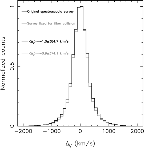
Figure 2: Velocity offset (relative to group centre) distribution before and after fixing the fiber collision issue.

4 Group Properties

In this section we briefly describe the procedures adopted for estimating group properties, such as velocity dispersion, physical radius ($R_{200}$), mass ($M_{200}$), and substructure. Further details can be found in Lopes et al. (2009a). These parameters are considered when studying the dependence of the FP on the environment.

4.1 Virial Analysis

For the virial analysis, first we compute the line-of-sight velocity dispersion ($\sigma_{P}$) of all group members within the aperture R_A (the radial offset of the most distant group member). R_A is normally close to the maximum radius ($R_{{\rm max}}=$ 4.0 Mpc), but could be much smaller in case the outermost galaxies are flagged as interlopers. The robust velocity dispersion estimate ($\sigma_{P}$) is given by the gapper or bi-weight estimator, depending on whether the number of galaxies available is $<15$ (gapper) or $\geq 15$ (bi-weight; Beers, Flynn, & Gebhardt 1990). Following the prescriptions of Danese, de Zotti, di Tullio (1980), the velocity dispersion is corrected for velocity errors. We also obtain an estimate of the projected “virial radius” R_PV (Girardi et al., 1998). A first estimate of the virial mass is given by (equation 5 of Girardi et al. 1998)

$${\rm M_{V}}={3\pi\sigma^{2}_{P}R_{PV}\over 2G},\,\,\,$$ (1)

where G is the gravitational constant and $3\pi/2$ is the de-projection factor.

Next we apply the surface pressure term correction to the mass estimate (The & White, 1986). To this effect, we need an estimate of the R₂₀₀ radius, which (as a first guess) is taken from the definition of Carlberg et al. (1997; equation 8 of that paper). We assume the percentage errors for the mass estimates are the same before and after the surface pressure correction (as in Girardi et al. 1998).

After applying this correction, we obtain a refined estimate of R₂₀₀ considering the virial mass density. If $M_{V}$ is the virial mass (after the surface pressure correction) in a volume of radius $R_{A}$, R₂₀₀ is then defined as R${}_{200}=R_{A}[\rho_{V}/(200\rho_{c}(z))]^{1/2.4}$. In this expression $\rho_{V}=3M_{V}/(4\pi R_{A}^{3})$ and $\rho_{c}(z)$ is the critical density at redshift $z$. The exponent in this equation is the one describing an NFW (Navarro, Frenk, & White, 1997) profile near R₂₀₀ (Katgert, Biviano, & Mazure, 2004). If we use five-hundred instead of two-hundred on this equation, we obtain an estimate of R₅₀₀. Next, assuming an NFW profile we estimate M₂₀₀ (or M₅₀₀) from the interpolation (most cases) or extrapolation of the virial mass M_V from R_A to R₂₀₀ (or R₅₀₀). Then, we use the definition of M₂₀₀ (or M₅₀₀) and a final estimate of R₂₀₀ (or R₅₀₀) is derived. This procedure is analogous to what is done by Popesso et al. (2007) and Biviano et al. (2006).

Fig. 3 shows, from top to bottom, the following distributions: N₂₀₀ (number of member galaxies within R₂₀₀); velocity dispersion (in km/s); R₂₀₀ (in Mpc); and M₂₀₀ ($10^{14}$ M_⊙). Note that, as expected from the FoF selection function, most systems are low richness and low mass systems. However, there are still 101 (112) clusters with velocity dispersion (mass) larger than $600\,kms^{-1}$ ($5\times 10^{14}M_{\odot}$). Six clusters have $\sigma_{P}>1000km/s$, with a maximum value of $1591\,kms^{-1}$.

In a forthcoming contribution of the SPIDER series, we will analyse the scaling relations of groups and clusters in the FoF catalogue (cf. Lopes et al. 2009b).

Figure 3: Distributions of N₂₀₀ (number of member galaxies within R₂₀₀), velocity dispersion (in km/s), R₂₀₀ (in Mpc), and M₂₀₀ ($10^{14}$ M_⊙). Notice that most of systems are poor groups, though there is a conspicuous number (101) of clusters with $\sigma_{P}$ higher than $600\,kms^{-1}$.

4.2 Substructure estimates

On what regards substructure, we employ a 3D substructure test to all FoF groups with at least five galaxy members within R₂₀₀. The DS, or $\Delta$ test (Dressler & Shectman, 1988), is applied as in Lopes et al. (2009a). The code used for the substructure analysis is the one from Pinkney et al. (1996), who evaluated the performance of thirty-one statistical tests.

The algorithm computes the mean velocity and standard deviation ($\sigma$) of each galaxy and its N_nn nearest neighbours, where N${}_{nn}=$ N^1/2 and N is the number of galaxies in the group region. Then these local mean and $\sigma$ values are compared with the global mean and $\sigma$ (based on all galaxies). For every galaxy, a deviation from the global value is defined by the formula below. Substructure is estimated with the cumulative deviation $\Delta$ (defined by $\sum\delta_{i}$; see below). For objects with no substructure we have $\Delta\sim$ N.

$${\rm\delta_{i}^{2}}=\left(\frac{N_{nn}+1}{\sigma^{2}}\right)[(\bar{v}_{local}-\bar{v})^{2}+(\sigma_{local}-\sigma)^{2}].\,\,\,$$ (2)

Any substructure test statistic has little meaning if not properly normalised, which can be achieved by comparing the results for the input data to those for substructure-free samples (the null hypothesis). For the $\Delta$ test the null hypothesis files are created after the velocities are shuffled randomly with respect to the positions, which remain fixed (Pinkney et al., 1996).

For each input data set, we generate five-hundred simulated realisations. We then calculate the number of Monte Carlo simulations which show more substructure than the real data. Finally, this number is divided by the number of Monte Carlo simulations. We set our significance threshold at 5$\%$, meaning that only twenty-five simulated data sets can have substructure statistics higher than the observations to consider a substructure estimate significant. Further details can be found in Pinkney et al. (1996), Lopes et al. (2006) and Lopes et al. (2009a).

For each FoF group the substructure test is applied to the 3D distribution of all galaxy members, as selected by the shifting-gapper method. The $\Delta$ test is only applied to systems with at least five galaxies available within R₂₀₀. Out of the 8,083 groups satisfying these criteria, we find that 3,570 ($\sim$ 44,2%) show significant signs of substructure. We note that this fraction is larger than found by Lopes et al. (2009a). That is probably due to the fact that (in order to correct for the fiber collision issue) we artificially assign redshifts to galaxies not targeted for spectroscopic observations.

We found that the fraction of groups with substructures increases from $\sim 30\%$ at $M_{200}\sim 10^{1}3M_{\odot}$ to $\sim 80\%$ for clusters as massive as $10^{14}M_{\odot}$. Notice that this result should be taken with caution, as low (relative to high) mass systems usually have a lower number of member galaxies and this might affect the efficiency in detecting substructures at the low mass regime .

5 The Environment of ETGs

5.1 Density Estimates

Galaxy density is estimated as follows. For each galaxy member of a given FoF group, we compute its projected distance, d_N, to the Nth galaxy of that group, where N = N${}_{memb}^{1/2}$, and N_memb is the number of member galaxies in the group. The local density $\Sigma_{N}$ is given by N/$\pi$d${}_{N}^{2}$, measured in units of galaxies/Mpc². The d_N is expressed in units of $Mpc$, using the redshift of the given group. For the density estimation we only consider member galaxies within a fixed luminosity range (see comments below). Notice that differently from other works density is not computed relative to all other galaxies in the field, but only relative to the other group members. Hence, instead of using $\Sigma_{5}$ or $\Sigma_{10}$, which are more common in the literature, we use $\Sigma_{N}$ so that the distance used for estimating density scales according to the number of members (or group mass). A further note is that if for a given galaxy there are fewer than N member neighbours (in the given luminosity range), we cannot compute the distance to the Nth galaxy of that group, d_N. In that case, $\Sigma_{N}$ is set to a lower limit of $0.01$. However, that only happens for about $0.1\%$ of the objects in the optical sample of ETGs with group membership.

In La Barbera et al. (2010b) (hereafter paper II), we showed that the sample of ETGs is complete to $M_{r}=-20.55$ for 2DPHOT total magnitudes. This corresponds to a limit of $M_{r}=-20.32$ for SDSS model magnitudes. Here we compute local density by (SDSS) petrosian magnitudes. The above limit translates to $M_{r}=-20.23$ for petrosian magnitudes. The density estimates are derived in the same luminosity range for all galaxies, no matter which FoF group they belong to. This limit is fixed by the maximum redshift of SPIDER ($z=0.095$). At this redshift, for petrosian magnitudes, the characteristic magnitude of the galaxy luminosity function is $M^{*}=-21.43$ in r band (Popesso et al. 2005). If we make $M^{*}+X=-20.23$, we find $X=1.2$. Hence, when deriving densities, we select only group members brighter than $M^{*}+1.2$.

Fig. 4 shows the comparison of $\Sigma_{N}$ computed with the original spectroscopic SDSS survey and after fixing it for the fiber collision issue (see section 2.2). In this Figure, we use dots to show the results for all galaxies for which density was estimated. Large green points show the median values for bins containing $5,000$ galaxies. As expected, the correction increases the $\Sigma_{N}$ value. The effect is slightly stronger at high $\Sigma_{N}$, the regime where we expected the fiber collision issue to be more relevant. Fig. 5 shows the density distribution for all member galaxies within the $8,083$ FoF groups. Galaxies residing in the FoF groups span a wide range of environments, corresponding to more than three decades in local galaxy density.

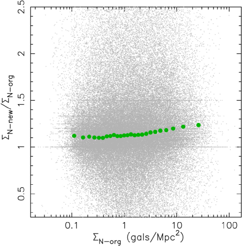
Figure 4: Comparison of $\Sigma_{N}$ computed with the original spectroscopic SDSS survey and after fixing it for the fiber collision issue. Dots are used for all the galaxies for which density is estimated. Large green points show the median values for bins containing 5000 galaxies each.

Figure 5: Distribution of local galaxy density ($\Sigma_{N}$) for all group members.

5.2 Definition of group and field galaxies

The environment of ETGs is first defined by the location of a galaxy in either a group or the field. For galaxies residing in groups, the environment is further characterized in terms of the group properties, such as the group-centric distance, mass, physical radius, and substructure. Group galaxies have also local density estimated relative to other group members (as described above), while for field galaxies, we use the FP relation itself to introduce a fictitious local density value (see Sec. 7.1).

Galaxies residing in groups are simply those having group membership according to the shifting gapper method (within $R_{{\rm max}}=$ 4.0 Mpc; see Sec. 3). Both the optical and optical+NIR samples of ETGs (Sec. 2) are cross-correlated to the list of galaxies belonging to groups, so that we define which SPIDER ETG has a parent group in the FoF updated catalogue.

Field ETGs are defined as follows. We start selecting only the ETGs that are not members of any group in the updated FoF catalogue. As reported in Sec. 3, because of the low number of galaxies available for some (poor) groups, we are able to measure group properties and define galaxy members for $79.2\%$ of the FoF groups. This implies that some galaxies with no assigned membership may still reside in one of the not-measured groups, and should be excluded from a genuine field sample. To clean the field sample from these cases, we check all the FoF groups (10,124 systems), removing those ETGs with radial offsets $<5\times R_{perp,rms}$ and velocity offsets $c\times\Delta_{z}<5\times\sigma_{v}$ from any group, where $R_{perp,rms}$ and $\sigma_{v}$ are the projected rms radius of the group and velocity dispersion as defined in the original FoF catalogue (Berlind et al., 2006). Galaxies on the border of a group in the phase-space diagrams (Fig. 1) can be not classified as group members by the shifting gapper technique, but nevertheless their properties might still be affected by the group because of the in-falling in its potential well. To remove this further source of $``contamination^{\prime\prime}$ from the field sample, we check once more all the 8,083 measured groups, removing objects with radial offsets $<5\times R_{200}$ and velocity offsets $c\times\Delta_{z}<5\times\sigma_{P}$ from any group, where $R_{200}$ and $\sigma_{P}$ are the characteristic radius and velocity dispersion of a group computed as described in Sec. 4. The remaining ETGs define the field sample.

Applying this procedure to the r-band sample of ETGs ($N=36,124$), we obtain two subsamples of $16,717$ group and $11,824$ field galaxies. For the optical+NIR sample of ETGs ($N=4,589$), the above selection results in $2,187$ group and $1,359$ field galaxies, respectively.

6 Measuring the FP relation

As in paper II, we write the FP relation as:

$$\log R_{\rm e}=a\log\sigma_{\rm 0}+b<\!\mu\!>_{\rm e}+c,$$ (3)

where ${}^{\prime\prime}a^{\prime\prime}$ and ${}^{\prime\prime}b^{\prime\prime}$ are the slopes, and ${}^{\prime\prime}c^{\prime\prime}$ is the offset (intercept) of the FP, $\log R_{\rm e}$  is the logarithmic effective radius of galaxies, in units of kpc, $<\!\mu\!>_{\rm e}$  is the mean surface brightness within that radius, and $\sigma_{0}$ is the central velocity dispersion. For the present study, we use $\sigma_{0}$ values from SDSS, although we verified that results are the same when using STARLIGHT velocity dispersions (see paper I). The $\sigma_{0}$’s are corrected to a circularised aperture of radius $r_{e}/8$, following Jørgensen, Franx, & Kjærgaard (1995). The computation of $\log R_{\rm e}$  and $<\!\mu\!>_{\rm e}$  in the different wavebands is described in detail in paper I. In general, we refer to ${}^{\prime\prime}a^{\prime\prime}$, ${}^{\prime\prime}b^{\prime\prime}$, and ${}^{\prime\prime}c^{\prime\prime}$, as the coefficients of the FP.

In order to analyse environmental effects on FP coefficients, we proceed as follows. In Sec. 7, we first compare the offset of the FP in different environmental bins. The values of $``c^{\prime\prime}$ for samples of ETGs in the different bins are computed by fixing the slopes of the FP to the values of $a=1.39$ and $b=0.315$ obtained in paper II for the entire SPIDER sample. This allows us to interpret differences in $``c^{\prime\prime}$ as differences in the average mass-to-light (hereafter $M/L$) ratio of ETGs among different environmental bins (Sec. 8). Notice that this FP-based $M/L$ ratio differs from the quantity $M_{dyn}/L$, where dynamical mass , $M_{dyn}\propto R_{e}\sigma_{0}^{2}$, and galaxy luminosity, $L$, are directly estimated from the data (see e.g. Bernardi et al. 2003a). The $``c^{\prime\prime}$ is measured as

$$c=\overline{\log R_{e}}-a\times\overline{\log\sigma_{0}}-b\times\overline{<\mu>_{e}},$$ (4)

where $\overline{\log R_{e}}$, $\overline{\log<\!\mu\!>_{e}}$, and $\overline{\log\sigma_{0}}$  are the median values of $\log R_{\rm e}$, $<\!\mu\!>_{\rm e}$, and $\log\sigma_{0}$. For a given sample of ETGs (i.e. a given environmental bin), the uncertainties on ${}^{\prime\prime}c^{\prime\prime}$ are computed by the width of the distribution of ${}^{\prime\prime}c^{\prime\prime}$ values, as computed by Eq. 4, from $1000$ bootstrap realisations of the sample. Since the values of ${}^{\prime\prime}a^{\prime\prime}$ and ${}^{\prime\prime}b^{\prime\prime}$ are kept fixed in Eq. 4 for all realisations, this procedure neglects the effect of the (correlated) uncertainties on ${}^{\prime\prime}a^{\prime\prime}$ and ${}^{\prime\prime}b^{\prime\prime}$. As discussed in Sec. 7, this further source of uncertainty can be completely neglected, as far as the difference of ${}^{\prime\prime}c^{\prime\prime}$ among different environments is concerned. The environmental variation of $``c^{\prime\prime}$ is used in Sec. 9 to properly measure the slopes of the FP for the ETG’s samples populating the different (environmental) bins. The values of $``a^{\prime\prime}$ and $``b^{\prime\prime}$ are estimated by an orthogonal robust fitting procedure and corrected for selection effects as well as the effect of correlated uncertainties on structural parameters (see paper II for details). We implement a procedure to account for the different average mass-to-light of galaxies in the different environmental bins, as well as the $``$luminosity segregation^′′ of galaxy populations with the environment (see Sec. 9 for details). The scatter of ETGs around the FP and its dependence on environment is not analysed here, being the subject of a forthcoming paper in this series.

7 The offset of the FP as a function of environment

We start analysing the dependence of the offset $``c^{\prime\prime}$ of the FP on galaxy environment. Sec. 7.1 presents the results obtained from the optical sample of ETGs, while the variation of “c” from $g$ through $K$ is analysed in Sec. 7.2.

7.1 The FP offset in r band

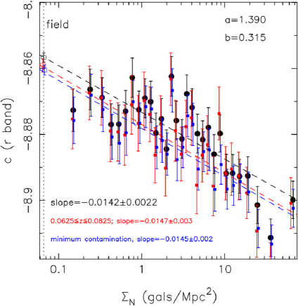
Figure 6: Variation of the offset $``c^{\prime\prime}$ of the FP as a function of local galaxy density, $\Sigma_{N}$. Filled circles plot the values of $``c^{\prime\prime}$ obtained binning the group sample of ETGs with respect to $\Sigma_{N}$, adopting 30 bins with the same number of galaxies each. Error bars denote $1~{}\sigma$ uncertainties. The $``c^{\prime\prime}$ has been computed by fixing $``a^{\prime\prime}$ and $``b^{\prime\prime}$ in all bins to the same values of $1.39$ and $0.315$, respectively, as shown in the upper-right corner of the figure. The dashed black line is the best-fit line to the filled circles, derived by a least-squares fitting procedure with $``c^{\prime\prime}$ as dependent variable. The slope value of the line is reported in the lower–left of the plot. The value of $``c^{\prime\prime}$ for the field sample of ETGs is also shown in the figure as an empty circle. The average local density value of field galaxies, marked by the vertical dotted line, is assigned by using the above linear fit (see the text). Red and blue squares are obtained by selecting only galaxies in a narrower redshift range and in the lower contamination sample of ETGs. The corresponding least-squares fits of $``c^{\prime\prime}$ versus $\log\Sigma_{N}$ are plotted by the red and blue dashed lines, whose slope values are reported in the lower–left of the Figure.

Fig. 6 plots the value of $``c^{\prime\prime}$ for the optical sample of ETGs, as a function of the local galaxy density $\Sigma_{N}$. The sample of group galaxies is binned with respect to $\Sigma_{N}$, with each bin including the same number of $557$ galaxies. This leads to $30$ density bins. The Figure shows that $``c^{\prime\prime}$ smoothly decreases from low to high density regions. A linear fit of this trend, with

$$c=a_{\Sigma_{N}}+b_{\Sigma_{N}}\log\Sigma_{N},$$ (5)

gives $a_{\Sigma_{N}}=-8.8734\pm 0.0018$ and $b_{\Sigma_{N}}=-0.014\pm 0.002$. The value of $b_{\Sigma_{N}}$ differs from zero at $\sim 7$ $\sigma$, meaning that the variation of $``c^{\prime\prime}$ with $\Sigma_{N}$ is highly significant. The quantity $b_{\Sigma_{N}}$ represents the variation of $``c^{\prime\prime}$ per decade of local galaxy density, and encodes all the information about the dependence of the FP offset on the (local) environment (see Sec. 8). For the field sample of ETGs, an estimate of the local density is not available. Hence, we assign a fictitious $\Sigma_{N}$ value, $\Sigma_{field}$, to all the field ETGs. To this aim, we first compute the $``c^{\prime\prime}$ for the field sample. Then, inverting Eq. 5, with $a_{\Sigma_{N}}$ and $b_{\Sigma_{N}}$ given by the values listed above, we infer the $\Sigma_{field}$ value.

Table 1: Covariance matrix terms of the uncertainties on $a$, $b$, $a_{\Sigma_{N}}$, and $b_{\Sigma_{N}}$.

$X$	$Y$	$C(X,Y)$
$a$	$a$	$4.150e-04$
$a$	$b$	$9.964e-06$
$a$	$a_{\Sigma_{N}}$	$-1.515e-03$
$a$	$b_{\Sigma_{N}}$	$-2.900e-06$
$b$	$b$	$1.970e-06$
$b$	$a_{\Sigma_{N}}$	$-7.462e-05$
$b$	$b_{\Sigma_{N}}$	$-3.499e-08$
$a_{\Sigma_{N}}$	$a_{\Sigma_{N}}$	$6.378e-03$
$a_{\Sigma_{N}}$	$b_{\Sigma_{N}}$	$7.565e-06$
$b_{\Sigma_{N}}$	$b_{\Sigma_{N}}$	$5.137e-06$

A possible source of concern in the trend of $``c^{\prime\prime}$ with environment is the contamination of the SPIDER samples from galaxies with non-genuine early-type morphology (see paper I). Due to the morphology-density relation (Dressler, 1980), these objects are expected to be more abundant in the low density regions. To analyse the impact of such contamination, in paper I we have defined a low contamination sample of ETGs consisting of $32,650$ (out of $39,993$) galaxies. For each bin of local density, we select only galaxies in this low contamination subsample. The resulting trend of $``c^{\prime\prime}$ with local density is shown by the blue symbols in the Figure. Besides a rigid shift, the slope of the trend is identical to that obtained with the entire sample, proving that contamination does not affect at all our results. Another source of concern is the redshift range of the SPIDER sample. Fainter galaxies are relatively more abundant in the lower density regions, and are better represented in the low redshift tail of the sample. Due to small evolutionary effects in the luminosity of ETGs (e.g. Bernardi et al. 2003a), this effects can bias the trend of the offset with the environment. To tackle with this issue, we select in all the environmental bins only galaxies in a narrower redshift bin, from $z=0.0625$ to $z=0.0825$. The corresponding trend of $``c^{\prime\prime}$ with local density is shown by the red symbols in Fig. 6. The slope of the $``c^{\prime\prime}$–$\log\Sigma_{N}$ fit is fully consistent with that of the entire sample.

We find that the $``c^{\prime\prime}$–$\log\Sigma_{N}$ trend is robust with respect to the statistical estimator used to calculate the FP intercept. Replacing the median values of $\log R_{\rm e}$, $<\!\mu\!>_{\rm e}$  and $\log\sigma_{0}$, in Eq. 4 with the peak values of the distributions, as estimated by the bi-weight estimator (Beers, Flynn, & Gebhardt, 1990), we obtain a very similar trend, whose slope, $b_{\Sigma_{N}}$, is indistinguishable from that reported in Fig. 6. Since the bi-weight (relative to the median) estimator is less sensitive to the shape of the tails in the distribution being analysed, this test also shows that the trend of $``c^{\prime\prime}$ with $\log\Sigma_{N}$ is not affected by the different shape of the massive end of the galaxy luminosity function in different environments, i.e. the larger fraction of bright galaxies inhabiting higher (relative to lower) density environments. Notice that the values of $``c^{\prime\prime}$ in different bins of $\log\Sigma_{N}$ are measured by keeping the values of FP slopes, $``a^{\prime\prime}$ and $``b^{\prime\prime}$, fixed (Sec. 6). On the other hand, as shown in Sec. 9, the FP slopes show a small, but significant trend with the environment, which might bias the $``c^{\prime\prime}$–$\log\Sigma_{N}$ trend. In order to address the issue, we recomputed the $``c^{\prime\prime}$ by setting $a=2$ and $b=0.4$ in Eq. 3. This corresponds to measure the mass-to-light ratio of ETGs by means of the virial theorem, rather than the FP equation, hence avoiding the possible $``degeneracy^{\prime\prime}$ between the environmental variation of FP slopes and intercept. Setting $a=2$ and $b=0.4$, the trend of $``c^{\prime\prime}$ with $\log\Sigma_{N}$ turns out to be fully consistent with that shown in Fig. 6, with the slope of the best-fitting line amounting to $-0.02\pm 0.004$ (compared to $-0.014\pm 0.002$). More in general, we verified that all the environmental trends of $``c^{\prime\prime}$ remain statistically unchanged when using either the FP or the virial theorem equation.

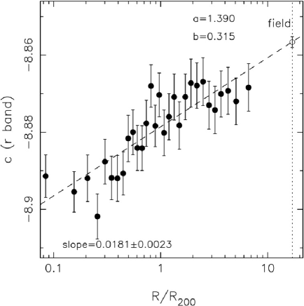
Figure 7: Same as Fig. 6 but plotting “c” as a function of the normalised cluster-centric distance $R/R_{200}$. The trend of increasing “c” with $R/R_{200}$ closely reflects the one shown in Fig. 6 for the local galaxy density. Notice that the field sample is also plotted in the Figure as an empty circle. The cluster-centric distance, $R_{field}/R_{200}$, is assigned to field galaxies in the same way as the local galaxy density, $\Sigma_{field}$ (see the text).

The error bars in Fig. 6 deserve further comment. As stated in Sec. 6, we compute the uncertainties on ${}^{\prime\prime}c^{\prime\prime}$ by keeping ${}^{\prime\prime}a^{\prime\prime}$ and ${}^{\prime\prime}b^{\prime\prime}$ fixed in Eq. 4. This corresponds to neglect the effect of (correlated) errors of ${}^{\prime\prime}a^{\prime\prime}$ and ${}^{\prime\prime}b^{\prime\prime}$ on the error bars of ${}^{\prime\prime}c^{\prime\prime}$ in Fig. 6, and hence on the estimated uncertainty on $b_{\Sigma_{N}}$. To analyse the effect of the errors on ${}^{\prime\prime}a^{\prime\prime}$ and ${}^{\prime\prime}b^{\prime\prime}$, we adopt the following approach. We take the covariance matrix of the uncertainties on ${}^{\prime\prime}a^{\prime\prime}$ and ${}^{\prime\prime}b^{\prime\prime}$, as estimated by the orthogonal fitting procedure (see paper II), and perform $1000$ iterations, shifting each time the values of ${}^{\prime\prime}a^{\prime\prime}$ and ${}^{\prime\prime}b^{\prime\prime}$ according to their correlated errors. For each iteration, the values of ${}^{\prime\prime}c^{\prime\prime}$ in all the environmental bins of Fig.7 are re-computed, together with the values of $a_{\Sigma_{N}}$ and $b_{\Sigma_{N}}$. Notice that in a given bin of $\Sigma_{N}$, the ${}^{\prime\prime}c^{\prime\prime}$ is computed by extracting a bootstrap realisation of the galaxy sample in that bin. We then estimate the covariance matrix of the values of ${}^{\prime\prime}a^{\prime\prime}$, ${}^{\prime\prime}b^{\prime\prime}$, $a_{\Sigma_{N}}$, and $b_{\Sigma_{N}}$, among the different iterations. The uncertainties provided by this covariance matrix account for both the scatter around the FP, as already given by the error bars in Fig. 7, as well as the correlated errors on FP slopes. All terms of the covariance matrix, $C(X,Y)$, where $X$ ($Y$) is one of the quantities ${}^{\prime\prime}a^{\prime\prime}$, ${}^{\prime\prime}b^{\prime\prime}$, $a_{\Sigma_{N}}$, and $b_{\Sigma_{N}}$, are reported in Tab. 1. The root square of the terms $C(a,a)$ and $C(b,b)$ are the uncertainties on ${}^{\prime\prime}a^{\prime\prime}$ and ${}^{\prime\prime}b^{\prime\prime}$ in r-band (cf. tab. 6 of paper II). The 1 $\sigma$ uncertainty on $b_{\Sigma_{N}}$ amounts to $\sim 0.0023$, being given by the root square of $C(b_{\Sigma_{N}},b_{\Sigma_{N}})$($=5.137e-06$). This uncertainty is indistinguishable from the value of $0.0022$ reported in Fig. 7, where the uncertainty on $b_{\Sigma_{N}}$ was estimated by neglecting the uncertainties on ${}^{\prime\prime}a^{\prime\prime}$ and ${}^{\prime\prime}b^{\prime\prime}$. In other words, as far as the environmental trend of ${}^{\prime\prime}c^{\prime\prime}$ is concerned (i.e. the value of $b_{\Sigma_{N}}$), the effect of the errors on ${}^{\prime\prime}a^{\prime\prime}$ and ${}^{\prime\prime}b^{\prime\prime}$ can be completely neglected, and the dominant source of error is the rms of residuals around the FP. Notice also that the covariance term between $b_{\Sigma_{N}}$ and ${}^{\prime\prime}a^{\prime\prime}$ is negative, implying that as ${}^{\prime\prime}a^{\prime\prime}$ increases the value of $b_{\Sigma_{N}}$ tends to become smaller. The same holds for the covariance term $C(b,b_{\Sigma_{N}})$. This is consistent with the fact that, when fixing the values of ${}^{\prime\prime}a^{\prime\prime}$ and ${}^{\prime\prime}b^{\prime\prime}$ to the virial theorem expectations, we obtain a value of $b_{\Sigma_{N}}$ slightly smaller, but still statistically consistent (see above), than that reported in Fig. 7..

Fig. 7 plots the $``c^{\prime\prime}$ in r band as a function of the median cluster-centric distance of ETGs to their parent groups. Cluster-centric distances are normalised to the corresponding $R_{200}$ values, allowing a meaningful comparison of galaxies residing in groups having different physical radii. The $``c^{\prime\prime}$ significantly increases from about $-8.9$ in the very central cluster regions, $R/R_{200}\sim 0.1$, to about $-8.865$ in the group’s outskirts ($R/R_{200}\sim 7$). The range of variation is very similar to that found for local density, implying that both trends are providing the same kind of information. It is interesting to notice that the linear fits of $``c^{\prime\prime}$ vs. $\log\Sigma_{N}$ and $R/R_{200}$ have very similar rms values, amounting to $0.009\pm 0.001$ and $0.008\pm 0.001$, respectively. Notice that Fig. 7 also plots the value of $``c^{\prime\prime}$ for the field sample. To this aim, a fictitious cluster-centric distance, $R_{field}/R_{200}$, is assigned to field galaxies, using the linear fit of $``c^{\prime\prime}$ versus $R/R_{200}$, in the same way as for $\Sigma_{field}$ (see above).

Figure 8: Same as Fig. 6 but plotting “c” as a function of the mass of the parent group where galaxies reside. The field sample is not shown in the plot.

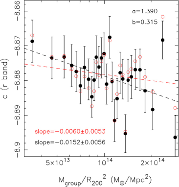
Figure 9: Same as Fig. 6 but plotting “c” as a function of the projected mass density, $M_{group}/R_{200}^{2}$, of the parent groups where ETGs reside. Red circles are the values of $``c^{\prime\prime}$ corrected for the expected amount of variation of $``c^{\prime\prime}$ among the different bins due to the different local density of galaxies in them. The corresponding best-fit line is shown by the red dashed line. Its slope value is reported in the lower–left of the plot.

Fig. 8 plots the $``c^{\prime\prime}$ as a function of the median mass value, $M_{group}$, of the groups where galaxies reside. We find that the offset of the FP decreases as the parent halo mass increases. The variation is significant at the 3 $\sigma$ level, as shown by the linear fit of $``c^{\prime\prime}$ versus $M_{group}$, whose slope value, $0.053\pm 0.018$, is reported in the same Figure. The variation of $``c^{\prime\prime}$ with group mass is much weaker than those found for $R/R_{200}$ and $\Sigma_{N}$. This is also shown in Fig. 9, where we plot the $``c^{\prime\prime}$ as a function of the projected mass density, $M_{group}/R_{200}^{2}$, of parent groups. This plot can be more directly compared to the variation with local density $\Sigma_{N}$. The FP offset tends to decrease as the $``global^{\prime\prime}$ density increases. However, in the latter case, the variation is much weaker than that with $\Sigma_{N}$. Using Eq. 5, we can correct the values of $``c^{\prime\prime}$ in the different bins of $M_{group}/R_{200}^{2}$, removing the expected variation due to the different median value of $\Sigma_{N}$ of galaxies in them. The corrected points are shown as red circles in the Figure. The trend of $``c^{\prime\prime}$ with $``global^{\prime\prime}$ mass density disappears, proving that the environmental variation of the FP intercept is essentially driven by $\Sigma_{N}$. In other terms, local environment turns out to be the main driver of differences in FP offset.

In order to further analyse this point, we derive the variation of $``c^{\prime\prime}$ with density for different bins of $M_{group}$. The r-band sample of ETGs is binned simultaneously with respect to $\Sigma_{N}$ and $M_{group}$, with a total of 64 bins, each bin including the same number of 261 galaxies. Fig. 10 plots the $``c^{\prime\prime}$ as a function of $\Sigma_{N}$ for different bins of group mass. The “c” tends to decrease as $\Sigma_{N}$ increases in all mass bins. Each trend is modelled by a linear fit as in Fig. 6 (see Eq. 5), and compared to the linear fit obtained for the entire sample (dot–dashed lines in the Figure). The slope value, $b_{\Sigma_{N}}$, of the $``c^{\prime\prime}$ vs. $\log\Sigma_{N}$ relation tends to become progressively steeper from poor groups to rich clusters. In fact, the $b_{\Sigma_{N}}$ value changes from about $-0.005$ for $M_{group}\sim 0.1\times 10^{14}M_{\odot}$ to about $-0.023$ for $M_{group}\sim 5.8\times 10^{14}M_{\odot}$. For comparison, the slope of the $``c^{\prime\prime}$ – $\log\Sigma_{N}$ relation for the entire r-band sample is $b_{\Sigma_{N}}=-0.014\pm 0.002$ (see Fig. 6). Fig. 11 plots the $b_{\Sigma_{N}}$ as a function of the median group mass $M_{group}$. A simple linear fit shows that the steepening of $``c^{\prime\prime}$ – $\log\Sigma_{N}$ relation with group mass is significant at the $2.5~{}\sigma$ level.

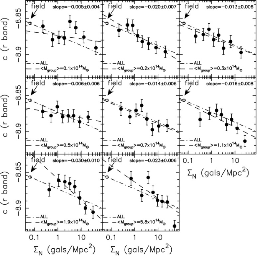
Figure 10: Offset $``c^{\prime\prime}$ of the FP as a function of local galaxy density for different bins of parent group mass, $M_{group}$. Each panel is the same as Fig. 6 but plotting only the FP offset for ETGs in a given bin of $M_{group}$. The median value of $M_{group}$, $<\!M_{group}\!>$, increases from left to right and top to bottom, being reported in the lower–left corner of each panel. The dashed lines are the linear fits of “c” vs. $\log\Sigma_{N}$, with their slope values being reported in the upper part of each panel. The dot–dashed line is the same for all panels, and corresponds to the best-fitting line of “c” vs. $\log\Sigma_{N}$ for the entire r-band sample. It coincides with the dashed black line in Fig. 6.

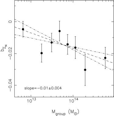
Figure 11: Slope of the $``c^{\prime\prime}$ vs. $\log\Sigma_{N}$ relation, $b_{\Sigma_{N}}$, as a function of the median mass of parent groups where ETGs reside. The slope of the best-fit line (dashed line in the plot) is reported in the lower–left part of the plot. The slope value differs from zero at the $2.5~{}\sigma$ significance level. The dot–dashed lines mark the $\pm 1$ $\sigma$ confidence levels around the best-fit.

7.2 The FP offset from g through K

Using the optical+NIR sample of ETGs, we derive the variation of the FP offset as a function of environment, from the $g$ through the $K$ band. We bin the optical+NIR sample of group galaxies with respect to $\Sigma_{N}$, each bin including the same of number of $273$ galaxies. This results into a total of eight bins. For a given bin, the $``c^{\prime\prime}$ is computed from Eq. 4, using the same sample of galaxies in all wavebands. Fig. 12 plots the FP offset as a function of $\Sigma_{N}$ from $g$ through $K$. The values of $``c^{\prime\prime}$ for the optical+NIR sample of field galaxies are also shown in the Figure, adopting the $\Sigma_{N}$ value ($\Sigma_{field}$) derived for field galaxies in Sec. 7.1. The $``c^{\prime\prime}$ smoothly decreases from low to high density regions, with all wavebands showing the same trend. In order to characterise the trends, we fit the data in each band with a linear relation:

$$c=a_{{}_{\Sigma_{N},X}}+b_{{}_{\Sigma_{N},X}}\log\Sigma_{N},$$ (6)

with $X=grizYJHK$. The fit is done by a least-squares method, with $``c^{\prime\prime}$ as dependent variable. The uncertainties on fitting coefficients are estimated by $N=500$ bootstrap iterations, shifting the values of $``c^{\prime\prime}$ according to their uncertainties. The best-fit values of $a_{{}_{\Sigma_{N},X}}$ and $b_{{}_{\Sigma_{N},X}}$ are reported in Tab. 2. Notice that the variation of $``c^{\prime\prime}$ per decade in local density, i.e. the $b_{{}_{\Sigma_{N},X}}$, are fully consistent, within the corresponding uncertainties, among the available wavebands. The values of $a_{{}_{\Sigma_{N},r}}$ ($=-8.8713\pm 0.0024$) and $b_{{}_{\Sigma_{N},r}}$ ($=-0.0097\pm 0.0027$) are fully consistent with those derived for the optical sample of ETGs, i.e. $a_{\Sigma_{N}}=-8.8734\pm 0.0018$ and $b_{\Sigma_{N}}=-0.014\pm 0.002$ (see Sec. 7.1). We do not attempt here to derive the $``c^{\prime\prime}$ as a function of both $\Sigma_{N}$ and $M_{group}$. In fact, due to the smaller sample size of the optical+NIR sample of ETGs, binning the $``c^{\prime\prime}$ with respect to both $\Sigma_{N}$ and $M_{group}$ would overly reduce the sample size in each bin.

Table 2: Coefficients of the linear fits to the trend of $``c^{\prime\prime}$ with local density in different wavebands.

waveband	$a_{{}_{\Sigma_{N},X}}$	$b_{{}_{\Sigma_{N},X}}$
$g$	$-9.1452\pm 0.0030$	$-0.0124\pm 0.0034$
$r$	$-8.8713\pm 0.0024$	$-0.0097\pm 0.0027$
$i$	$-8.8244\pm 0.0025$	$-0.0096\pm 0.0027$
$z$	$-8.7134\pm 0.0026$	$-0.0108\pm 0.0025$
$Y$	$-8.5496\pm 0.0027$	$-0.0098\pm 0.0028$
$J$	$-8.5357\pm 0.0026$	$-0.0080\pm 0.0028$
$H$	$-8.3709\pm 0.0027$	$-0.0119\pm 0.0030$
$K$	$-8.2286\pm 0.0027$	$-0.0153\pm 0.0030$

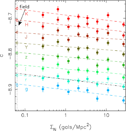
Figure 12: Dependence of the FP offset on local galaxy density in the $grizYJHK$ wavebands. Different wavebands are plotted with different colours, as shown by the labels below the dashed lines in the left part of the plot. Galaxies in the optical+NIR samples of ETGs residing in groups are binned according to $\Sigma_{N}$, with each bin including the same number of galaxies. For each bin, the $``c^{\prime\prime}$ is derived for the same sample of galaxies from $g$ through $K$. The values of $``c^{\prime\prime}$ for the field sample (empty circles) are reported in the same figure, adopting the local density value assigned to field galaxies from the linear fit in Fig. 6 (see Sec. 7.1). The dashed lines are the linear fits to the trend of $``c^{\prime\prime}$ with $\Sigma_{N}$ in each band. Error bars denote $1~{}\sigma$ uncertainties. Notice that suitable shifts have been applied to the values of $``c^{\prime\prime}$ in different bands to better display all the trends in the same plot.

8 Stellar population properties of ETGs in different environments

Using the virial theorem, one can rewrite the equation of the FP as a power-law relation between the mass-to-light ratio of ETGs and two other variables, such as the mass $M$, luminosity $L$, $\sigma_{0}$, $R_{e}$, and mean surface brightness (see paper II). The intercept of the FP turns out to be proportional to the mean $M/L$ ratio of ETGs at a given point of the galaxy sequence, parametrised in terms of the two adopted variables. Hence, the strong variation of $``c^{\prime\prime}$ with local environment, (Sec. 7.1 and Sec. 7.2), can be actually interpreted as a variation of $M/L$ with environment. Such a variation can be due to a change of $M$, $L$, or both quantities with $\Sigma_{N}$. In order to analyse this point, we plot in Fig. 13 the peak value of the quantity $\log R_{e}-a\log\sigma_{0}$, i.e. the combination of $\log R_{\rm e}$  and $\log\sigma_{0}$  that enters the FP, as a function of local galaxy density, for the r-band sample of ETGs. The peak value is computed by using the bi-weight estimator. We see no significant trend with respect to $\Sigma_{N}$, implying that the trend of $``c^{\prime\prime}$ is due to a variation of mean surface brightness with local density. Fig. 14 also plots the quantity $\log R_{e}+2\log\sigma_{0}$, which is a proxy for the galaxy dynamical mass, $M$, as a function of $\Sigma_{N}$. Even in this case, no variation with the environment is detected. This suggests that the $``c^{\prime\prime}$–$\log\Sigma_{N}$ relation origins from a change in the average luminosity, i.e. stellar population content, of ETGs as a function of environment, rather than a variation of galaxy mass (see also Sec. 10). The optical and NIR data can help us to further constrain the origin of such variation in stellar content. Assuming for simplicity that the variation of $M/L$ with environment can be entirely ascribed to age and metallicity, we write the following equations:

$$b_{{}_{\Sigma_{N},X}} = \frac{\delta c_{X}}{\delta\log\Sigma_{N}}=-\frac{\delta\log M/L_{X}}{\delta\log\Sigma_{N}}$$ (7)

$$= -\frac{\delta\log M_{\star}/L_{X}}{\delta\log t}\times\frac{\delta\log t}{\delta\log\Sigma_{N}}+$$

$$- \frac{\delta\log M_{\star}/L_{X}}{\delta\log Z}\times\frac{\delta\log Z}{\delta\log\Sigma_{N}},$$

where $M/L_{X}$ ($M_{\star}/L_{X}$) is the dynamical (stellar) mass-to-light ratio in the waveband $X$ ($=grizYJHK$), the quantities $c_{t,X}=\delta\log M_{\star}/L_{X}/\delta\log t$ and $c_{Z,X}=\delta\log M_{\star}/L_{X}/\delta\log Z$ are the partial derivatives of $M_{\star}/L_{X}$ with respect to the age $t$ and metallicity $Z$. Since $\delta\log M/L_{X}=\delta\log M/M_{\star}+\delta\log M_{\star}/L_{X}$, Eq. 7 assumes that, on average, the quantity $\log M/M_{\star}$, i.e. the average fraction of dark- to stellar-matter in ETGs, does not change significantly with the environment. As discussed in Sec. 10, this assumption is supported by the fact that the typical dynamical-mass of the ETGs in our sample does not change significantly with environment (see Fig. 14), and a variation of $M_{\star}$, at fixed $M$, is unlikely.. The quantities $\delta\log t/\delta\log\Sigma_{N}$ and $\delta\log Z/\delta\log\Sigma_{N}$ represent the variation of age and metallicity per decade in local galaxy density, and are the parameters we aim to constrain. We estimate the quantities $c_{t,X}$ and $c_{Z,X}$ as detailed in La Barbera & de Carvalho (2009) and paper II. In short, we construct several simple stellar population (SSP) models with the  Bruzual & Charlot (2003) synthesis code. All models have a Scalo IMF, and different ages and metallicities. Age values span a range of $\sim 8$ to $\sim 13$ Gyr, while metallicity varies from $0.2$ to $2.5Z_{\odot}$. For each model (i.e. each age and metallicity), we compute the mass-to-light ratios, $M_{\star}/L_{X}$, by folding the corresponding SED with the $grizYJHK$ filter curves. For each band, the values of $M_{\star}/L_{X}$ from the different models are fitted with an eight order polynomial in $\log t$ and $\log Z$. The rms of the fitting is smaller than a few percent in all the bands. The polynomial fits provide a simple, analytic tool to calculate the derivatives $c_{t,X}$ and $c_{Z,X}$ for an SSP model with given age and metallicity. In practise, we solved Eqs. 7 by evaluating the derivatives at an age of $10Gyr$ and solar metallicity. We verified that the results are very insensitive to the choice of such age and metallicity values. Moreover, using different stellar population models, as described in paper II, does not change at all the results. Eqs. 7 were solved in a least-squares sense, using the estimated values of $c_{t,X}$ and $c_{Z,X}$, and the values of $b_{{}_{\Sigma_{N},X}}$ from Tab. 2. In order to estimate the uncertainties on the solutions, $\delta\log t/\delta\log\Sigma_{N}$ and $\delta\log Z/\delta\log\Sigma_{N}$, we repeat the procedure by shifting the $b_{{}_{\Sigma_{N},X}}$’s according to their uncertainties.

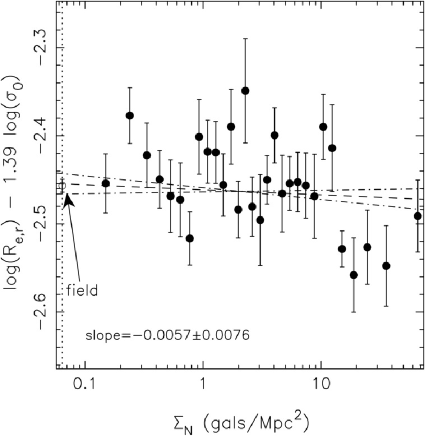
Figure 13: The peak value of the $\log R_{e}-a\log\sigma_{0}$ distribution, computed by the bi-weight statistics, is plotted as a function of local galaxy density for the samples of ETGs in groups (filled circles) and the field sample (empty circle). The field sample is marked by the vertical dotted line. The best-fitting line to the data is plotted as a dashed line. The dot–dashed lines mark the $\pm 1~{}\sigma$ confidence levels on the best-fit relation.

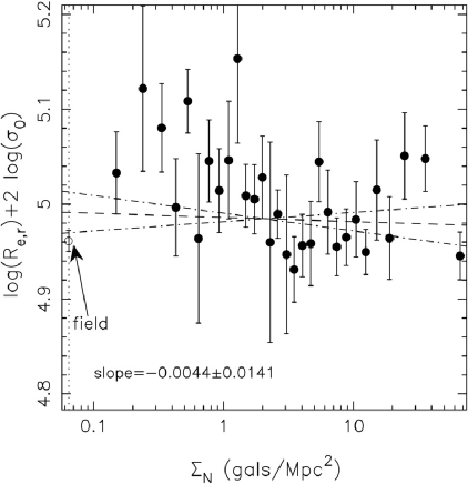
Figure 14: Same as Fig. 13 but for the quantity $\log R_{e,r}+2\log\sigma_{0}$, which is a proxy for galaxy dynamical mass.

Fig. 15 plots the $b_{{}_{\Sigma_{N},X}}$ as a function of the effective wavelength of the filter $X$, from $g$ through $K$. The solid curve is obtained by inserting the best-fitting solutions, $\delta\log t/\delta\log\Sigma_{N}$ and $\delta\log Z/\delta\log\Sigma_{N}$, into Eq. 7, and computing the expected values of $b_{{}_{\Sigma_{N},X}}$. We see that a combined variation of age and metallicity is able to match very well the value of $b_{{}_{\Sigma_{N},X}}$ in all wavebands. The dashed and dotted curves in the Figure are obtained with the same procedure by setting either $\delta\log Z/\delta\log\Sigma_{N}=0$ or $\delta\log t/\delta\log\Sigma_{N}=0$ in Eq. 7. They correspond to pure age and metallicity models of the variation of $``c^{\prime\prime}$ with local density. The pure metallicity model is clearly inconsistent with the observations. In fact, a difference in metallicity would tend to produce a negligible difference of mass-to-light ratios in K-band, as the NIR light is very insensitive to differences in metallicity, through line-blanketing. On the other hand, a pure age model is still able to match the observations, but with a large discrepancy, of $\sim 2~{}\sigma$, in K-band.

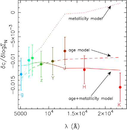
Figure 15: Variation of the FP intercept per decade in local galaxy density as a function of the effective wavelength of each filter (out of $grizYJHK$). The solid, dashed, and dotted curves are age+metallicity, pure age, and pure metallicity stellar population models (see the text). Each waveband is indicated by a different colour, as shown by the labels beneath the error bars.

Fig. 16 plots the values of $\delta\log t/\delta\log\Sigma_{N}$ vs. $\delta\log Z/\delta\log\Sigma_{N}$ obtained from the procedure described above. The scatter in the plot (black dots) reflects the measurement uncertainties on the quantities $b_{{}_{\Sigma_{N},X}}$. As expected from the fact that $\delta\log Z/\delta\log\Sigma_{N}$ and $\delta\log t/\delta\log\Sigma_{N}$ are estimated from the same system of equations (Eqs. 7), the measurement errors on $b_{{}_{\Sigma_{N},X}}$ imply a correlated variation of $\delta\log Z/\delta\log\Sigma_{N}$ and $\delta\log t/\delta\log\Sigma_{N}$. A linear fitting of the $\delta\log Z/\delta\log\Sigma_{N}$ and $\delta\log t/\delta\log\Sigma_{N}$ values (dashed line) gives a slope of $-4.36\pm 0.05$. Taking the mean and standard deviation of $\delta\log Z/\delta\log\Sigma_{N}$’s and $\delta\log t/\delta\log\Sigma_{N}$’s, we obtain ‘$\delta\log Z/\delta\log\Sigma_{N}=-0.043\pm 0.023$ and $\delta\log t/\delta\log\Sigma_{N}=0.048\pm 0.006$, i.e. ETGs in higher density regions are older, by $\sim 11\%$ per decade in local density, and less metal-rich than galaxies at low density. We notice that the value of $\delta\log Z/\delta\log\Sigma_{N}$ is consistent with zero at about $2~{}\sigma$, implying that, as noticed above, a pure age model might be able by itself to explain the observations. For a pure age model, the average value of $\delta\log t/\delta\log\Sigma_{N}$ reduces to $0.04\pm 0.004$, rather than $0.048\pm 0.006$.

In Sec. 7, we have reported some evidence that the variation of $``c^{\prime\prime}$ per decade in local density is stronger for galaxies residing in more massive (relative to poor) clusters. As shown in Fig. 11, for $M_{group}\widetilde{>}2\times 10^{14}M_{\odot}$, the absolute value of $b_{{}_{\Sigma_{N}}}$ is about twice larger than that of $-0.0097$ reported in Tab. 2. For a pure age model, from Eq. 7, one would infer that, for more massive clusters, the variation in age per decade of local galaxy density is around twice larger than that reported above, i.e. $\delta\log t/\delta\log\Sigma_{N}\sim 0.08$.

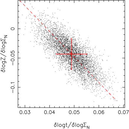
Figure 16: Variations of age and metallicity per decade in local galaxy density, $\delta\log t/\delta\log\Sigma_{N}$ and $\delta\log Z/\delta\log\Sigma_{N}$, implied by the variation of the FP offset with $\log\Sigma_{N}$ in the different wavebands. The best solutions of Eq. 7 are marked by the red circle. The black points are the values of $\delta\log t/\delta\log\Sigma_{N}$ and $\delta\log Z/\delta\log\Sigma_{N}$ obtained by shifting the $b_{{}_{\Sigma_{N},X}}$ according to the corresponding uncertainties. The dashed line is obtained by an ordinary least-squares fitting procedure, taking the arithmetic average of the results obtained by changing the role of the dependent variable in the fitting.

9 Slopes of the FP as a function of the environment

So far we have analysed the offset of the FP, interpreting it as a difference of the average mass-to-light ratio of ETGs residing in different environments. In this section, we study the dependence of $``a^{\prime\prime}$ and $``b^{\prime\prime}$ themselves on environment. In Sec. 9.1, we analyse the slopes $``a^{\prime\prime}$ and $``b^{\prime\prime}$ in the r band, taking advantage of the large size of the optical ETG’s sample. In Sec. 9.2, we derive the waveband dependence of FP slopes.

9.1 The slopes of the FP in r band

We start comparing the slopes of the FP for the r-band samples of field and group galaxies (Sec. 5.2). To this aim, we have to account for two different effects, (i) field galaxies have on average lower mass-to-light ratios than those in groups (see Sec. 8), and (ii) ETGs are characterized by a luminosity segregation, for which brighter ( i.e. higher $L$) galaxies mostly inhabit the denser cluster regions. Moreover, not only $L$, but also galaxy radii are expected to change with environment, as they correlate with position within cluster (e.g. Cypriano et al. 2006). Point (i) implies that, at a given mass, an ETG in a lower density region is on average brighter than a galaxy with the same mass, but in a denser environment. Moreover, even removing this effect, the relative distribution of galaxy luminosities and mean surface brightnesses might depend on environment (point ii). To account for points (i) and (ii), we proceed as follows. First, we fix the slopes of the FP, as in Sec. 7.1, and derive the intercepts of the FP for the field and group samples. From Eq. 4, the average luminosity difference between the two samples is given by $\delta E=-(\delta c)/b=-0.077\pm 0.007$ mag. Then, we shift the $<\!\mu\!>_{\rm e}$  values of galaxies in the field sample by $-\delta E$, and bin both the field and group samples with respect to total magnitude and mean surface brightness. For each bin, we randomly extract the same number of field and group galaxies. This procedure, described in detail in paper II (see the app. B), allows us to extract two subsamples of field and group galaxies having the same distribution in the space of the effective parameters. By construction, both subsamples consist of the same number of galaxies, i.e. $N=11,024$ out of $11,824$ and $16,717$ ETGs in the field and groups, respectively. It follows that any difference in the FP slopes for these two subsamples arises from the different ways velocity dispersions are related to the effective parameters, rather than from any spurious ($``geometric^{\prime\prime}$) effect due to different relative fraction of galaxies in different regions of the parameter space. In other words, we are “removing” the dependence of galaxy luminosities and radii on environment, in order to measuring the genuine dependence of the FP on environment.

Fig. 17 plots the $``a^{\prime\prime}$ and $``b^{\prime\prime}$ values for the field and group subsamples. We find a significant difference between the FP of field and group galaxies, with field galaxies having higher $``a^{\prime\prime}$ and lower $``b^{\prime\prime}$ value. For the ${}^{\prime\prime}a^{\prime\prime}$, the difference is significant at $\sim 3~{}\sigma$. Notice that had we not homogenised the luminosity and $<\!\mu\!>_{\rm e}$  distributions of galaxies in the two samples, we would have found an almost negligible difference in $``a^{\prime\prime}$ (at $\sim 1\sigma$), and a stronger difference in $``b^{\prime\prime}$ (at $\sim 5~{}\sigma$). The dependence of galaxy luminosities and radii on environment plays an important role. If not accounted for, it would lead to underestimating the dependence of the coefficient ${}^{\prime\prime}a^{\prime\prime}$ on environment. To further test this result, we have implemented a procedure to wash out the dependence of FP on environment and measure only the effect that the environmental dependence of galaxy luminosities and radii have on FP coefficients. For a given galaxy parameter (e.g. luminosity), we bin the sample of field+group galaxies with respect to that parameter, each bin including the same number of $N=100$ galaxies. Then, we scramble the galaxy environments, preserving the number of objects residing in each environmental bin (i.e. field and groups). The resulting shuffled sample is split again into field and group galaxies. Since both galaxy luminosities and radii are known to be affected from environments (see above), we perform the scrambling with respect to both $L$ and $r_{e}$. Also, we consider the case of scrambling $<\!\mu\!>_{\rm e}$  (as it reflects both $L$ and $r_{e}$) and the remaining FP variable, $\log\sigma_{0}$. The FP slopes of the scrambled samples of field and group galaxies are reported in Tab. 3. The coefficient ${}^{\prime\prime}b^{\prime\prime}$ is fully consistent between the scrambled samples of field and group galaxies. For the ${}^{\prime\prime}a^{\prime\prime}$, we see that scrambling $<\!\mu\!>_{\rm e}$  and $\log\sigma_{0}$, does not impact at all its dependence on environment. On the other hand, scrambling $L$ and $r_{e}$ has the net effect of decreasing ($by\sim 5\%$) the ${}^{\prime\prime}a^{\prime\prime}$ for field (relative to group) galaxies. This result is fully consistent with our conclusion above. Field galaxies have higher ${}^{\prime\prime}a^{\prime\prime}$ than group galaxies. However, the dependence of $L$ and $r_{e}$ on environment does not make this difference immediately detectable, as it tends to decrease ${}^{\prime\prime}a^{\prime\prime}$ for the field sample.

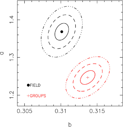
Figure 17: Slopes $``a^{\prime\prime}$ and $``b^{\prime\prime}$ of the FP for field (black circle) and group (red cross) galaxies. The solid, dashed, and dot–dashed ellipses mark the $1,~{}2$ and $3~{}\sigma$ confidence contours on $``a^{\prime\prime}$ and $``b^{\prime\prime}$, respectively. Notice that both the field and group samples have the same distribution in the space of the effective parameters (after the average difference in mass-to-light ratio is accounted for), and include the same number of $11,024$ ETGs (see the text).

Table 3: FP slopes of ETGs in groups and field obtained by scrambling galaxy environment at fixed size, surface brightness, velocity dispersion, and logarithmic luminosity.

scrambling	field		groups
	$a$	$b$	$a$	$b$
$r_{e}$	$1.350\pm 0.019$	$0.315\pm 0.001$	$1.406\pm 0.014$	$0.316\pm 0.001$
$<\!\mu\!>_{\rm e}$	$1.399\pm 0.016$	$0.315\pm 0.001$	$1.388\pm 0.016$	$0.316\pm 0.001$
$\log\sigma_{0}$	$1.401\pm 0.017$	$0.315\pm 0.001$	$1.391\pm 0.014$	$0.316\pm 0.001$
$\log L$	$1.353\pm 0.020$	$0.314\pm 0.001$	$1.402\pm 0.014$	$0.316\pm 0.001$

We derive the FP slopes of ETGs residing in groups with and without substructures. The presence of substructures is characterized by a 3D $\Delta$ test (see Sec. 4.2). About $44\%$ of groups show evidence of substructures. ETGs in the optical sample are first split in two subsamples according to the presence ($N=9133$) or not ($N=7584$) of substructures in the parent groups. Notice that although less than half of the groups have substructures, there is a large number of ETGs residing in groups with substructures. Then, proceeding as described above, we extract two subsamples of galaxies with the same distribution in the space of effective parameters. These subsamples include $7,716$ galaxies each. No correction for the average mass-to-light ratio is applied, as we obtain similar values of the FP offset for the two samples, i.e. $c=-8.876\pm 0.002$ and $c=-8.882\pm 0.002$ for the case with and without substructures, respectively. Fig. 18 compares the FP slopes for the two $``homogenised``$ subsamples. The corresponding values of ${}^{\prime\prime}a``$ and ${}^{\prime\prime}b``$ are fully consistent.

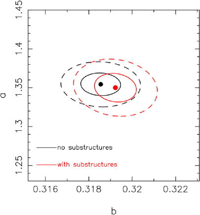
Figure 18: Slopes $``a^{\prime\prime}$ and $``b^{\prime\prime}$ of the FP for galaxies residing in groups with (red) and without (black) substructures. The solid and dashed ellipses mark the $1$ and $2~{}\sigma$ confidence contours on $``a^{\prime\prime}$ and $``b^{\prime\prime}$, respectively.

To compare the FP slopes of galaxies residing in different bins of local density, we apply the same binning procedure used to characterise the trend of $``c^{\prime\prime}$ with $\Sigma_{N}$ (Fig. 6). To derive the slopes of the FP in each bin, we proceed in a similar way as in the comparison of field and group galaxies, i.e. we account for (i) the different average mass-to-light ratio of ETGs in different environmental bins, and (ii) differences in the relative distribution of galaxies in the space of effective parameters. First, we estimate the average luminosity difference of galaxies residing in different bins with respect to the field sample, using the linear fit of $``c^{\prime\prime}$ versus $\log\Sigma_{N}$ (Eq. 5). For a given density bin, $i$, the average luminosity difference is given by

$$\delta E_{i}=-\frac{b_{{}_{\Sigma_{N}}}\times(\log\Sigma_{N}-\log\Sigma_{field})}{b},$$ (8)

where $\Sigma_{field}$ is the local density value assigned to field galaxies (Sec. 7.1). We then shift the $<\!\mu\!>_{\rm e}$  values of the entire optical sample of ETGs by $\delta E_{i}$, and extract a subsample of galaxies with the same luminosity and $<\!\mu\!>_{\rm e}$  distributions as galaxies in the $i$-th $\Sigma_{N}$ bin. We compute the relative variations, $\delta a/a$ and $\delta b/b$, of the FP slopes of the entire sample after these selections are applied. The factors $\delta a/a$ and $\delta b/b$ are applied to the FP slopes of galaxies in the given local density bin. By construction, the correction vanishes for the field sample, while it become more and more important as $\Sigma_{N}$ increases. Fig. 19 plots the r-band slopes of the FP as a function of local galaxy density. In order to characterise the trend of $``a^{\prime\prime}$ and $``b^{\prime\prime}$ with $\Sigma_{N}$, linear fits of both slopes with respect to $\log\Sigma_{N}$ are performed. Notice that the field sample is not included in the fit.

In general, one can notice that the FP slopes exhibit only a weak dependence on environment. Before applying any correction, the $``a^{\prime\prime}$ does not show any variation with $\Sigma_{N}$, with the slope of the linear regression ($0.00\pm 0.03$; see Fig. 19) being fully consistent with zero. After the corrections are applied, we are able to detect a $2.5~{}\sigma$ tendency of $``a^{\prime\prime}$ to decrease from low to high density environments. One can notice that, in agreement with this trend, the corrected value of $``a^{\prime\prime}$ for the field sample is larger than all the slope values obtained for the higher density subsamples ($\Sigma_{N}>1gals/Mpc^{2}$). This is consistent with what found above, when comparing the FP slopes of field and group galaxies (Fig. 17). Notice that the values of $``a^{\prime\prime}$ and $``b^{\prime\prime}$ in Fig. 17 refer to a different sample of field galaxies with respect to that considered in Fig. 19. In fact, for Fig. 17, two subsamples of field and group galaxies are extracted, to match the corresponding distributions of galaxies in the space of structural parameters. For the comparison in Fig. 19, the FP slopes are derived by using all galaxies in the field sample. This explains the difference (in absolute value) of the values of $``a^{\prime\prime}$ and $``b^{\prime\prime}$ for field galaxies between Fig. 17 and Fig. 19. Despite that, the relative difference of FP coefficients between the field and group samples are detected in both cases. The coefficient $``b^{\prime\prime}$ tends to increase with local galaxy density. The correction procedure shows that the tendency is significant at $\sim 3\sigma$, and is mostly due to galaxies in higher density regions ($\Sigma_{N}\widetilde{>}10\,gals\,Mpc^{-2}$). As shown in Fig. 20, the trends of $``a^{\prime\prime}$ and $``b^{\prime\prime}$ with environment become weaker when plotting their value as a function of the normalised cluster-centric distance $R/R_{200}$. In this case, the corrections are estimated with the same approach described above, using the fictitious value of the cluster-centric distance of the field sample ($R_{field}/R_{200}$) and the linear fit of $``c^{\prime\prime}$ versus $R/R_{200}$ (see Fig. 7). We find that the $``b^{\prime\prime}$ increases from the centre to the periphery of galaxy groups, as expected from the variation of $``b^{\prime\prime}$ with local galaxy density. For the $``a^{\prime\prime}$, we do not detect any significant variation with $R/R_{200}$.

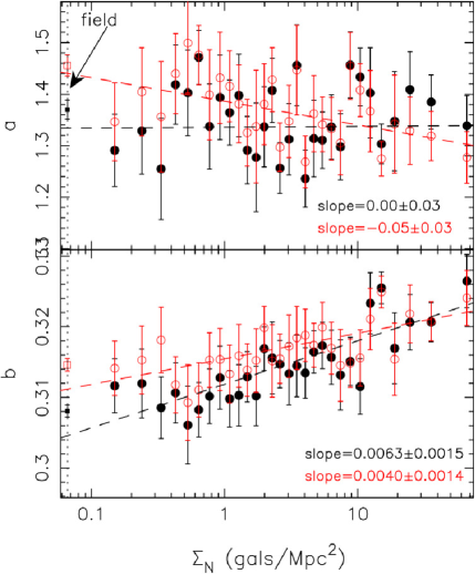
Figure 19: The slopes $``a^{\prime\prime}$ and $``b^{\prime\prime}$ of the FP are plotted as a function of local galaxy density, $\Sigma_{N}$. Error bars denote $1~{}\sigma$ uncertainties. Red colour shows the case where the slopes are corrected for the environmental dependence of the average mass-to-light ratio of ETGs and luminosity segregation of galaxies in different environments (see the text). The dashed lines are the linear least-squares fits to the data points. The squares in the left part of the plots are the slope’s values for the field sample, as also indicated by the vertical dotted line and the arrow.

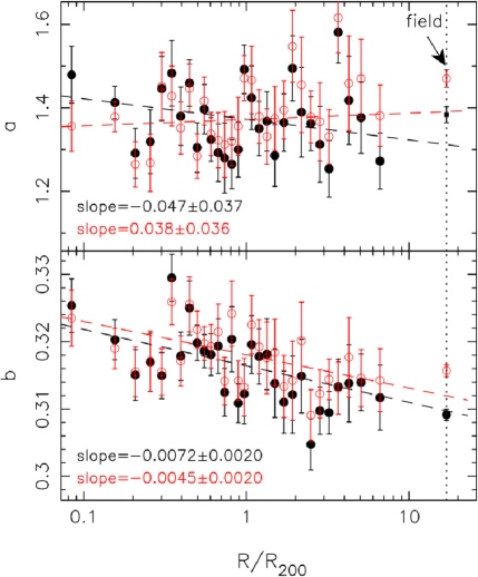
Figure 20: The same as Fig. 19 but plotting the $``a^{\prime\prime}$ and $``b^{\prime\prime}$ as a function of the normalised distance to the centre of the parent groups where galaxies reside.

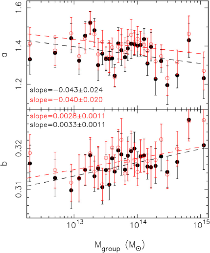
Figure 21: The same as Fig. 19 but plotting the $``a^{\prime\prime}$ and $``b^{\prime\prime}$ as a function of mass of parent groups where galaxies reside.

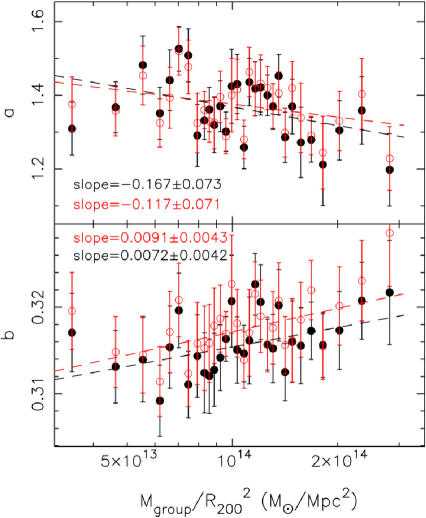
Figure 22: The same as Fig. 19 but plotting the $``a^{\prime\prime}$ and $``b^{\prime\prime}$ as a function of $``global^{\prime\prime}$ surface mass density, $M_{group}/R_{200}^{2}$, of the parent groups where galaxies reside.

Fig. 21 plots the FP slopes in r band as a function of the mass of the parent galaxy groups. As for $\Sigma_{N}$ and $R/R_{200}$, we plot the values of $``a^{\prime\prime}$ and $``b^{\prime\prime}$ with and without the corrections for the effects (i) and (ii) mentioned above. We find that the coefficient $``a^{\prime\prime}$ tends to decrease (at $\sim 2~{}\sigma$) for galaxies residing in more massive clusters, while the $``b^{\prime\prime}$ shows an opposite and more significant (at $\sim 3~{}\sigma$) trend, increasing for higher $M_{group}$. A similar result is obtained when characterising the global environment in terms of the $``global^{\prime\prime}$ projected mass density, $M_{group}/R_{200}^{2}$, of the parent galaxy groups. The $``a^{\prime\prime}$ ($``b^{\prime\prime}$) exhibits only a weak trend to decrease (increase) with $M_{group}/R_{200}^{2}$ (Fig. 22). As shown by the slope values of the linear fits, the trends of $``a^{\prime\prime}$ and $``b^{\prime\prime}$ with $``global^{\prime\prime}$ density are only marginally significant, at less than $2~{}\sigma$. On the contrary, the dependence on local density seems to be more significant, as shown by the uncertainties on the slope values reported in Fig. 19. This implies that the local rather than the global environment is the main driver of the environmental dependence of the slopes of the FP. The same result has been shown to hold for the offset of the FP (Sec. 7.1).

As for the $``c^{\prime\prime}$, we also analyse how the slopes of the FP depend on local galaxy density in different bins of mass of the parent galaxy groups. Figs. 23 and 24 plot the $``a^{\prime\prime}$ and $``b^{\prime\prime}$ as a function of $\log\Sigma_{N}$, in different bins of $M_{group}$. The binning is performed in the same way as for Fig. 10. The slope values are corrected as in Fig. 19. Fig. 23 does not show any significant dependence of $``a^{\prime\prime}$ on local galaxy density for all bins of $M_{group}$. This result is not necessarily inconsistent with the trend of $``a^{\prime\prime}$ with $\Sigma_{N}$ shown in Fig. 19 (upper panel), as binning the sample with respect to both $M_{group}$ and $\Sigma_{N}$ decreases the sample size in each bin, possibly washing out the ($2.5~{}\sigma$) environmental trend in Fig. 19. Fig. 24 shows that $``b^{\prime\prime}$ does not depend significantly on group mass for low mass groups, while it increases significantly with $\log\Sigma_{N}$ in the high mass regime. In the bin of highest $M_{group}$ ($5.8\times 10^{14}M_{\odot}$), the slope of the $``b^{\prime\prime}$–$\log\Sigma_{N}$ linear fit is significantly positive, at more than $4~{}\sigma$, for the case where no correction is applied, and at more than $2.5~{}\sigma$, when the correction is performed. We conclude that the dependence of $``b^{\prime\prime}$ on local density (Fig. 19) is mainly driven by galaxies residing in most massive clusters.

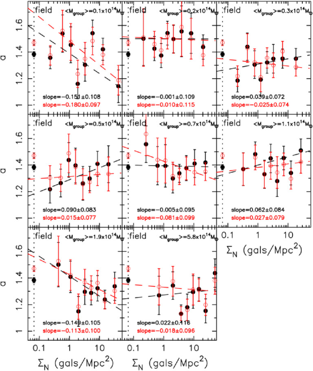
Figure 23: Dependence of the slope $``a^{\prime\prime}$ of the FP as a function of local density, $\Sigma_{N}$, in different bins of mass of the parent galaxy group. Red colour refers to the values of the slope after correcting for differences in the FP intercept and distribution in the space of structural parameters (see the text). Error bars denote $1~{}\sigma$ uncertainties. For each panel, the corresponding median value of the mass of the parent galaxy group, $<M_{group}>$, is reported in the upper-right. The $<M_{group}>$ increases from left to right, and top to bottom. The values of $``a^{\prime\prime}$ for the field sample are reported in each panel, and are marked by the vertical dashed line. The dashed lines are best-fit linear relations to the data points, with the corresponding slope values being reported in the lower-left part of each panel. Notice that the $\Sigma_{N}$ bins are the same as in Fig. 10.

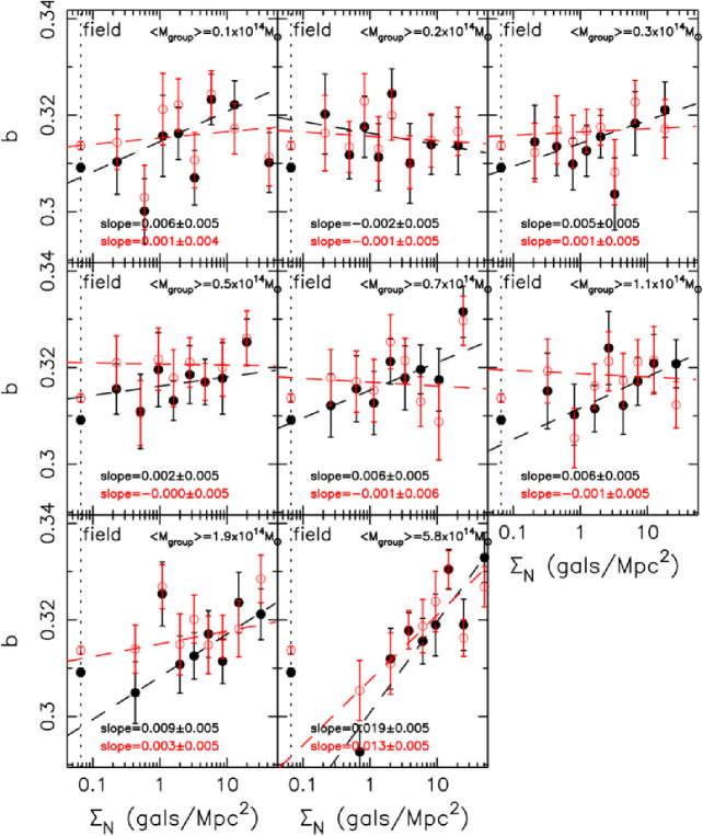
Figure 24: The same as Fig. 23 but for the coefficient $``b^{\prime\prime}$ of the FP.

9.2 The slopes of the FP from g through K

The environmental analysis of the waveband dependence of the FP involves essentially two aspects. We derive the relative variation of FP slopes, from $g$ through $K$, and compare such variation among different environmental bins. Since the waveband variation of FP slopes informs on how stellar population properties (i.e. age and metallicity) vary with galaxy mass (see paper II for details), this allows us to analyse how such stellar population variation is affected by the environment where galaxies reside. Moreover, as the NIR light closely follows the stellar mass distribution in galaxies and the contribution of stellar populations to the tilt of the FP in K-band vanishes (see paper II), the NIR (K-band) FP informs on how the ratio of dynamical to stellar mass (and/or the non-homology) of ETGs vary with mass, and how this variation is related to the environment. The results presented below are discussed, with regard to both aspects, in Sec. 10.2.

In order to derive the FP coefficients in different environments, we use the optical+NIR sample of ETGs, binning galaxies with respect to different environmental properties, and deriving the FP slopes in each bin. In all cases, the binning is performed as for the environmental analysis of the FP intercept from $g$ through $K$ (Sec. 7.2). We correct the FP slopes for the same effects mentioned in Sec. 9.1, i.e. environmental differences in the average mass-to-light and luminosity segregation. To this effect, we follow the same recipes as for the analysis of FP slopes in r-band (Sec. 9.1).

Fig. 25 plots the slopes of the FP from $g$ through $K$ for galaxies residing in groups and in the field. The optical+NIR samples of group and field galaxies consist of $2,185$ and $1,359$ galaxies, respectively. The upper panel of the Figure shows the FP slopes for these samples: we only detect a significant difference in the value of $b$ between field and group galaxies, with the latter having lower $``b^{\prime\prime}$ in all wavebands. However, to perform a proper comparison, we have to account for differences in mass-to-light ratio and luminosity segregation. To this effect, we proceed as for the comparison of field and group galaxies in the r band (see Sec. 9.1), by extracting two subsamples of galaxies with the same distributions in the space of structural parameters. This selection leads to field and group sub-samples with $1,264$ galaxies each. The corresponding FP slopes, from $g$ through $K$ are shown in the lower panel of Fig. 25. We are now able to detect also a difference in the coefficient $``a^{\prime\prime}$. The $``a^{\prime\prime}$ turns out to be smaller for group, relative to field, galaxies in all wavebands, in agreement with the result for the r-band samples (Fig. 17). In order to measure the variation of FP slopes from $g$ through $K$, we assume a linear relation between the $``a^{\prime\prime}$ ($``b^{\prime\prime}$) and the effective wavelength ($\lambda$) of each waveband, i.e.

$$a(\lambda) = p_{a}+q_{a}\log\lambda$$ (9)

$$b(\lambda) = p_{b}+q_{b}\log\lambda,$$ (10)

where $p_{a}$ ($p_{b}$) and $q_{a}$ ($q_{b}$) are the intercept and slope of the linear relation. The values of $p_{a}$ and $q_{a}$ ($p_{b}$ and $q_{b}$) are derived by an ordinary least-squares fit of $``a^{\prime\prime}$ ($``b^{\prime\prime}$) versus $\log\lambda$. The uncertainties on $p_{a}$ and $q_{a}$ ($p_{b}$ and $q_{b}$) are estimated from those on $``a^{\prime\prime}$ and $``b^{\prime\prime}$, accounting for the correlated errors of FP slopes among different wavebands . We find that, for all the subsamples of ETGs analysed in the present paper, Eqs. 9 and 10 are able to describe the trends of $``a^{\prime\prime}$ and $``b^{\prime\prime}$ with waveband with an accuracy of a few percent. They provide simple, empirical relations to quantify the waveband variation of FP slopes. For both field and group ETGs (lower panel of Fig. 25), we use Eqs. 9 and 10 to calculate the relative variation of $``a^{\prime\prime}$ and $``b^{\prime\prime}$ from $g$ through $K$, i.e.

$$\delta a_{g->K} = \frac{a(\lambda_{K})-a(\lambda_{g})}{a(\lambda_{g})}$$ (11)

$$\delta b_{g->K} = \frac{b(\lambda_{K})-b(\lambda_{g})}{b(\lambda_{g})}$$ (12)

where $\lambda_{g}$ and $\lambda_{K}$ are the effective wavelengths of the $g$ and $K$ passbands, respectively. The values of $\delta a_{g->K}$  and $\delta b_{g->K}$  define a segment in the $``a^{\prime\prime}$–$``b^{\prime\prime}$ plane, whose size quantifies the amount of variation of FP slopes from the optical to NIR. The segments corresponding to the subsamples of field and group ETGs, as well as the values of $\delta a_{g->K}$  and $\delta b_{g->K}$, are shown in the lower panel of Fig. 25. The uncertainty on $\delta a_{g->K}$  ($\delta b_{g->K}$) is obtained from those on $p_{a}$ and $q_{a}$ ($p_{b}$ and $q_{b}$). In general, the variations of $``a^{\prime\prime}$ and $``b^{\prime\prime}$ from $g$ through $K$ are similar for both samples. For the $``b^{\prime\prime}$, field galaxies tend to have a marginally steeper variation, with $\delta b_{g->K}$$=2.5\pm 0.7\%$, compared to $\delta b_{g->K}$$=1.1\pm 0.7\%$ for group galaxies. More in general, one can notice that while the $``a^{\prime\prime}$ is always smaller for group relative to field galaxies, the difference in $``b^{\prime\prime}$ between the two samples tends to vanish when moving from $``g^{\prime\prime}$ to $``K^{\prime\prime}$ (Sec. 9.1). To further quantify these differences, we take the average of the g- and r-band coefficients, and compare them to the mean values of $``a^{\prime\prime}$ and $``b^{\prime\prime}$ in the $JHK$ (NIR) wavebands. For the field (group) sample, the $``b^{\prime\prime}$ changes from $0.302\pm 0.003$ ($0.312\pm 0.002$) in the optical to $0.311\pm 0.003$ ($0.316\pm 0.003$) in the NIR. Thus, the difference in $``b^{\prime\prime}$ between the field and group samples is significantly in the optical, while becomes consistent with zero in the NIR. For the field (group) sample, the $``a^{\prime\prime}$ changes from $1.35\pm 0.06$ ($1.23\pm 0.04$) in the optical to $1.53\pm 0.06$ ($1.42\pm 0.05$) in the NIR. Thus, the difference in $``a^{\prime\prime}$ between the field and group samples is essentially independent of waveband, with the $``a^{\prime\prime}$ being smaller (at $\sim 2~{}\sigma$), for the group relative to field sample in both the optical and NIR.

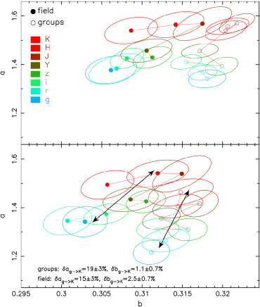
Figure 25: Slopes $``a^{\prime\prime}$ and $``b^{\prime\prime}$ of the FP from $g$ through $K$ for galaxies residing in groups (empty circles) and in the field (filled circles). Different colours correspond to different wavebands, as shown in the lower-left corner of the upper plot. Ellipses denote $1~{}\sigma$ confidence contours on $``a^{\prime\prime}$ and $``b^{\prime\prime}$. The upper and lower panels correspond to the cases where the FP coefficients are either corrected or not for the difference in the average mass-to-light ratio of galaxies in the different environments and the luminosity segregation effect. The black arrows in the lower panel plot the amount of relative variation from $g$ through $K$ of the FP slopes for the two subsamples, as obtained by assuming a power-law relation between the $``a^{\prime\prime}$ ($``b^{\prime\prime}$) and the effective wavelength of a given passband (see the text). The relative variations, $\delta a_{g->K}$  and $\delta b_{g->K}$, are reported in the lower–left part of the same panel.

Fig. 26 plots the FP slopes from $g$ through $K$ for galaxies residing in groups with and without substructures. We do not find any significant difference, for all wavebands, between the two samples.

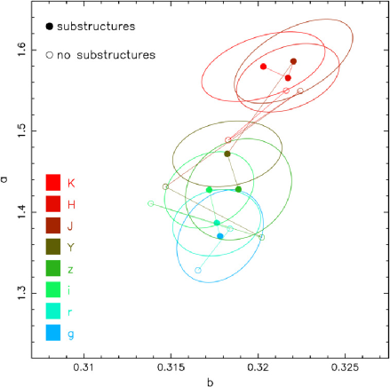
Figure 26: The same as the lower panel of Fig. 25 but for galaxies residing in groups with (filled circles) and without (empty circles) substructures.

Figs. 27 and 28 plot the slopes of the FP from $g$ through $K$ in different bins of local galaxy density, and mass of the parent galaxy groups. In each environmental bin, we apply suitable correction factors to the slope values, in order to account for environmental differences in the average mass-to-light and luminosity segregation. The corrections are computed as in the analysis of FP slopes in r-band (Sec. 9.1). For all wavebands, we apply the same corrections. This is justified by the fact that (a) we always analyse the same sample of ETGs in the different wavebands, and (b) as shown in Sec. 7.2 the amount of environmental variation of the FP offset is very similar in all wavebands, implying similar differences in the corresponding average mass-to-light ratios. We find that the waveband dependence of the FP is very similar in all wavebands. The $``a^{\prime\prime}$ tends to increase with wavelength in all environments. We measure the amount of end-to-end variation of $``a^{\prime\prime}$ and $``b^{\prime\prime}$, across the available wavelength baseline, by computing the quantities $\delta a_{g->K}$  and $\delta b_{g->K}$(see above). The value of $\delta a_{g->K}$  spans the range $\sim 11\%$ to $\sim 23\%$, with a weighted-mean value of $16\%$. All values of $\delta a_{g->K}$  are consistent within the errors with that of $16\pm 3\%$ measured for the field sample. The $``b^{\prime\prime}$ does not change significantly with waveband, with a marginal tendency to increase ($\delta b_{g->K}$$>0$) by $1$–$3\%$ from $g$ through $K$ in all the environments. Notice that the quantity $\delta b_{g->K}$  is positive in all bins of $\Sigma_{N}$ and $M_{group}$ with the exception of the the bin with highest value of parent group mass ($M_{group}=3.05\times 10^{14}\,M_{\odot}$, see Fig. 28). This is consistent with what shown in Fig. 25, i.e. the $``b^{\prime\prime}$ increases by a few percent with waveband for the field sample, while it is constant for galaxies in groups. Fig. 28 would also imply that this different behaviour is due to galaxies residing in massive clusters. The plots of $``a^{\prime\prime}$ and $``b^{\prime\prime}$ as a function of other environmental quantities, such as the cluster-centric distance and the $``global^{\prime\prime}$ mass surface density of the parent galaxy groups, do not add further information to the conclusions above, and are not shown here for brevity reasons.

To summarise, we find that the tilt of the FP, as measured by the coefficient $``a^{\prime\prime}$, is different between field and group galaxies, with group galaxies having lower $``a^{\prime\prime}$. The difference is independent of the passband where the galaxy structural parameters are measured. For the $``b^{\prime\prime}$, its variation with waveband is smaller than $\sim 3\%$. However, in this case, an important difference between field and group galaxies emerges, i.e. the $``b^{\prime\prime}$ increases with waveband (by $2.5\%$, see the value of $\delta b_{g->K}$  in Fig. 25), while for group galaxies the variation with waveband is insignificant. This seems to be especially true for galaxies residing in most massive clusters (Fig. 28), for which $\delta b_{g->K}$  is negative. The implications of these findings are discussed in Sec. 10.

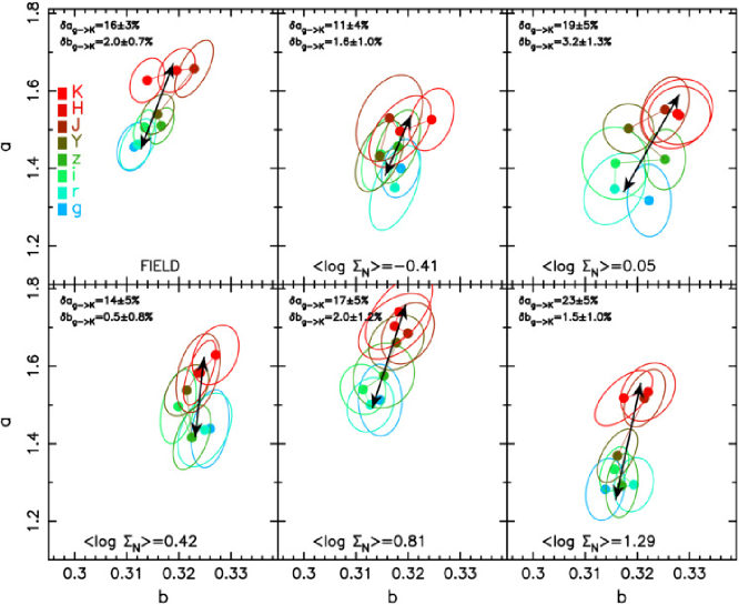
Figure 27: Slopes $``a^{\prime\prime}$ and $``b^{\prime\prime}$ of the FP in different bins of local galaxy density. The average value of $\log\Sigma_{N}$ in a given bin is reported in the lower part of the corresponding panel, increasing from left to right and top to bottom. The upper-left panel shows the results obtained for field galaxies. Ellipses denote the $1~{}\sigma$ confidence contours. For each panel, the segment shows the amount of variation of FP slopes from $g$ through $K$, obtained by a power-law fit of $``a^{\prime\prime}$ and $``b^{\prime\prime}$ as a function of the effective wavelength of each waveband. The amount of variations of $``a^{\prime\prime}$ and $``b^{\prime\prime}$, $\delta a_{g->K}$  and $\delta b_{g->K}$, are reported in the upper-left corner of each panel.

Figure 28: The same as Fig. 27 but for different bins of mass of parent galaxy groups.

10 Discussion

In the present work, we have analysed the environmental dependence of the FP coefficients on the waveband at which structural parameters are measured. On what follows, we discuss the environmental dependence of the FP in the optical (Sec. 10.1) and using the combined optical$+$NIR (Sec. 10.2). In Sec. 10.3 we examine the stellar content of ETGs in different environments. The most remarkable result we find here is the variation of the FP offset with local density. As shown in Sec. 8, this trend sets strong constraints on the variation of stellar population properties of ETGs with the environment. This point is discussed in Sec. 10.3.

10.1 Environmental dependence of the optical FP relation

The first attempt to measure systematic differences in the FP relation among different environments has been performed by de Carvalho & Djorgovski (1992) (hereafter dCD92; see also Djorgovski, de Carvalho, & Han ), who derived FP coefficients in the optical for a sample of $31$ cluster (mostly Coma and Virgo) and $34$ $``field^{\prime\prime}$ galaxies in the low-redshift-Universe. Field galaxies included also objects residing in poor and loose groups. The authors found that the offset $``c^{\prime\prime}$ of the FP for field galaxies is significantly different from that of galaxies in clusters. They interpreted qualitatively this difference as field galaxies being younger than those in clusters, consistent to what we find here. However, a direct and quantitative comparison of the values of $``c^{\prime\prime}$ between our study and dCD92 is not possible because of the different definition of environment and the different techniques used to estimate the FP intercept. Due to the uncertainties on FP coefficients, dCD92 did not detect any significant variation of FP slopes with environment.

The first systematic study of the FP relation in clusters, at optical wavebands, was performed by Jørgensen, Franx, & Kjærgaard (1996) (hereafter JFK96). They derived the FP coefficients for ETGs, in Gunn-r, residing in 11 nearby clusters (220 galaxies). They found no evidence for variation of FP coefficients with global cluster properties like richness, velocity dispersion and temperature of the intra-cluster gas. Also, they did not detect any correlation between residuals around the FP and the local environment, characterized as the cluster-centric distance and the projected cluster surface density (see also La Barbera, Busarello, & Capaccioli 2000). These results seem to contrast to what we find here, i.e. that both $``c^{\prime\prime}$ and (to minor extent) $``a^{\prime\prime}$ and $``b^{\prime\prime}$ depend on the environment (Secs. 7 and 9, respectively). However, one has to consider that the number of galaxies per cluster in JFK96 is much smaller (larger uncertainties) than that in each local density bin analysed here. For instance, looking at tab. 3 of JFK96, one can see that their typical error on $``b^{\prime\prime}$ varies from $\sim 0.02$ to $\sim 0.06$, among the different clusters, while in our case this error amounts on average to $\sim$0.006. The environmental variation of $``b^{\prime\prime}$ we find ranges from $\sim$0.02 to $\sim 0.04$ (see the panel representing the more massive systems in Fig. 24), comparable to the quoted uncertainties on $``b^{\prime\prime}$ in JFK96. This explains why we are able to detect such a small difference while JFK96 cannot.

Bernardi et al. (2006) (hereafter B06) analysed the offset of the FP relation of ETGs in low and high density regions (bins), using a large sample of ETGs from SDSS. The authors defined the environment using the C4 cluster catalogue (based on SDSS-DR2; see Miller et al. 2005). Galaxies were assigned to the high density bin using a cut in angular separation and radial velocity around each cluster, rather than assigning membership to each object as we do here (Sec. 5). Galaxies in the low density bin were defined using a cutoff in the maximum allowed distance for a $``field^{\prime\prime}$ galaxy to the n-th companion galaxy. This criterion was introduced by B06 in order to remove the contamination in the field sample from galaxies residing in poor and loose groups, which are likely not included in the C4 catalogue. On the contrary, the FoF catalogue we use here also includes poor galaxy groups, and we define the field sample according to the 3D distance of galaxies to the nearest group. Despite of these differences and the different sources of structural parameters used to derive the FP in the present study (i.e. 2DPHOT, see paper I) and B06 (i.e. the SDSS Photo pipeline), the difference of the FP intercept among field and group galaxies between our study and that of B06 is very consistent. In fact, the latter find that the average difference of $<\!\mu\!>_{\rm e}$  in r band, as derived from the FP, amounts to $0.075\pm 0.008$, with galaxies in denser regions having fainter surface brightness than their counterparts in the field. On the other hand, we find $-\delta c/b=0.077\pm 0.007$ mag (see Sec. 9.1), which is fully consistent with the B06 result. We address the implications of this result in Sec. 10.3.

A systematic study of the environmental effects on FP coefficients has been recently performed, in the optical, by D’Onofrio et al. (2008) (hereafter D08), in the framework of the WINGS project (Fasano et al., 2006). The sample of D08 consists of $1,550$ early-type galaxies in 59 massive clusters, in the low-redshift-Universe ($0.04<z<0.07$). Hence, they analyse a similar redshift range to that considered by our study, but with a different range in mass of the parent systems where galaxies reside. D08 detected no significant variation of FP coefficients with global cluster properties, such as richness, $R_{200}$, and velocity dispersion. On the contrary, we find evidence that the offset $``c^{\prime\prime}$ and (to minor extent) the slope $``b^{\prime\prime}$ of the FP change systematically with the global environment, with $``b^{\prime\prime}$ ($``c^{\prime\prime}$) increasing (decreasing) with respect to the parent group mass, $M_{group}$ (see Figs. 8 and 21). We notice that these trends are probably detectable only because of the larger range in $M_{group}$ spanned by our group/cluster catalogue (see Fig. 3) in comparison with theirs (400 $<$ $\sigma$ $<$ 1400 km/s, with $<\sigma>$ = 800 km/s).

Moreover, as discussed in Sec. 7, the trend with global environment can be entirely explained by the dependence of FP coefficients on local density. D08 found a strong variation of FP coefficients with the local environment. Both $``a^{\prime\prime}$ and $``b^{\prime\prime}$ were found to increase, and $``c^{\prime\prime}$ was found to decrease with respect to the (projected) local galaxy density. The trends of $``b^{\prime\prime}$ and $``c^{\prime\prime}$ from D08 are qualitatively consistent with those we find here (see Secs. 7.1 and 9.1). However, after correcting for systematic effects (see red circles in Fig. 19), we detect a $2.5\sigma$ indication that the $``a^{\prime\prime}$ decreases from the low to the higher density regions, in contrast with D08. Considering ETGs in the most massive groups (see Fig. 23), we still do not find any strong variation with local environment, as in D08. A possible explanation for this discrepancy can be the fact that we have corrected the FP slopes of different samples of ETGs for biases due to the environmental dependence of the average mass-to-light ratio of galaxies and the distribution of ETGs in the space of effective parameters, while D08 did not account for either effects. We also notice that the variation of $``b^{\prime\prime}$ with local environment from D08 is much larger than that detected here. From Fig. 19, we see that the end-to-end variation of $``b^{\prime\prime}$ with respect to local density amounts to less than $0.02$, while D08 find a variation of $\sim 0.04$ (see their fig. 15). This discrepancy can be explained by the different mass regime covered by our cluster sample and that of D08, and by the fact that we find the variation of $``b^{\prime\prime}$ with local environment to depend on the mass of parent galaxy groups. For groups as massive as $\sim 5.8\times 10^{14}\,M_{\odot}$, we find an end-to-end variation of $``b^{\prime\prime}$ of $\sim 0.04$ when none of the above corrections is applied (in agreement with D08). This variation reduces to $\sim 0.02$ after the corrections are performed.

10.2 Environmental dependence of the FP from g through K

For what concerns the waveband variation of FP coefficients, we find that the $``a^{\prime\prime}$ increases, by $\sim 16\%$, from $g$ through $K$, independent of the environment, while the variation of $``b^{\prime\prime}$ with passband is smaller than $\sim 3\%$. For field galaxies, (see Fig. 25), there is a $3~{}\sigma$ evidence that the $``b^{\prime\prime}$ increases, by $\sim 2.5\%$, from the optical to NIR, with the difference in $``b^{\prime\prime}$ between field and group galaxies vanishing in the NIR. For group galaxies, in particular those residing in most massive systems (Fig. 28), no variation of $``b^{\prime\prime}$ with waveband is detected. As discussed in paper II, the waveband dependence of FP slopes informs on the variation of stellar population properties with mass. For the entire SPIDER sample, the relative variation of $``a^{\prime\prime}$ and $``b^{\prime\prime}$ from $g$ through $K$ implies that ETGs, as a whole, have essentially coeval stellar populations, with metallicity being larger in more massive galaxies. As shown from eq. 7 of paper II, a smaller value of $``b^{\prime\prime}$ (as that we find here for field galaxies) implies a steeper variation of the mass-to-light ratio of ETGs along the galaxy (mass) sequence. As the $``b^{\prime\prime}$ increases from the optical to NIR for field galaxies, the corresponding mass-to-light ratio variation is related to the way stellar population properties change with mass. In other terms, the environmental variation of $``b^{\prime\prime}$ might imply that group galaxies exhibit a shallower relation between stellar population parameters (i.e. age and metallicity) and mass. Interestingly, this is consistent with the recent findings of Pasquali et al. (2010) (hereafter PGF10), who found that galaxies in denser environments have shallower age– and metallicity–mass relations. This is also a natural expectation of hierarchical models of galaxy formation, as galaxies in denser environments are those accreted in the group environment at earlier times, having their star formation quenched earlier through environmental-driven effects (e.g. strangulation), implying a shallower relation between (luminosity-weighted) age and stellar mass. A flatter metallicity–mass relation in denser environment might also result from the effect of tidal stripping on the more bound stellar material in galaxies (e.g. Klimentowski et al. 2009) as discussed by PGF10.
On the other hand, the difference in $``a^{\prime\prime}$ between field and group galaxies is the same at both optical and NIR wavebands. Group galaxies have a larger FP tilt, as measured by the coefficient $``a^{\prime\prime}$, likely because of a waveband-independent origin. A possible explanation is a different variation of dark-matter fraction and/or non-homology along the mass sequence of ETGs between galaxies in different environments. For instance, group galaxies might have a larger tilt because of a steeper relation between dark-matter fraction and mass, due to (i) tidal interactions between galaxy dark-matter halos and parent group halos, i.e. lower, relative to higher, mass galaxies are stripped more of their dark-matter halo as they fall into the cluster potential well; (ii) central galaxies have higher dark-matter fractions, as they acquire part of the dark-matter halo of the in-falling satellites. The first scenario might result from the fact that the total time span, during which galaxies are stripped, is larger for low mass galaxies (see e.g. eq. 9 of Cattaneo et al. 2010). However, tidal forces are stronger for more massive galaxies, as a short orbital decay time for $\rm L>L^{*}$ galaxies is expected (Barnes, 1989). The scenario (ii) might be more plausible, provided that stripped galaxies have mostly late-type morphology. This would not change significantly the peak value of dynamical mass of ETGs as a function of environment, consistent with Fig. 14, and increase only the dark-matter fraction for higher mass systems, implying a smaller tilt of the FP relation. Notice that a steeper relation between stellar to dynamical mass ratio and mass in ETGs for group (relative to field) galaxies has recently been suggested also from Shankar & Bernardi (2009), as a result of the wider range of luminosity-weighted ages characterizing cluster relative to field galaxies. These points will be further analysed in a forthcoming contribution in this series, using estimates of dynamical and stellar mass for ETGs and analysing their dependence on environment.

It is interesting to notice that the NIR FP, and its environmental dependence, can be connected to the stellar mass FP recently derived by Hyde & Bernardi (2009). The stellar mass FP is obtained by replacing luminosity (i.e. surface brightness) in the FP equation with stellar mass. Since the K-band light closely follows the stellar mass distribution in galaxies and the contribution of stellar populations to the tilt of the FP vanishes in the NIR (see paper II), the K-band FP should essentially coincide with the stellar mass FP. In fact, Hyde & Bernardi (2009) report a value of $a\sim 1.54\pm 0.02$ for the stellar mass FP, while we measure $a\sim 1.55\pm 0.02$ for the K-band FP. This reinforces the fact that the environmental difference of FP coefficients we detect in the NIR bands, among different environments (see above), implies an environmental difference in the relation between the ratio of dynamical-to-stellar mass and galaxy mass. Given the excellent agreement of the K-band and stellar mass FP’s, one might actually use either relations to derive ETG’s stellar masses, and test how realistic are the estimates from stellar population models.

10.3 Stellar content of ETGs in different environments

The environmental variation of the FP intercept, ‘$``c^{\prime\prime}$, implies that the average mass-to-light ratio of ETGs increases from low to high density regions. As seen in Eq. 7, this variation can be interpreted as a difference in the stellar content of ETGs, at fixed mass, provided that the ratio of dynamical to stellar mass, $M/M_{\star}$, does not increase, on average, with local density. There are several arguments against such an increase. First, Fig. 14 shows that the peak value of the quantity $\sigma_{0}^{2}\times R_{e}$ – a proxy for dynamical mass – does not change with the environment. So, the $M/M_{\star}$ can increase with local density, only if stellar mass, at fixed $M$, decreases with $\Sigma_{N}$. However, as galaxies are accreted into groups and clusters, they are expected to be stripped off of their dark-matter halos, resulting, eventually, into a larger $M_{\star}$, for fixed $M$, at high density. These arguments make plausible our assumption of constant $M/M_{\star}$, that allows us to use the offset of the FP as a tool to analyse the variation of stellar population properties as a function of environment. It is interesting to note that, as shown in fig. 8 of Bernardi et al. (2006), at fixed luminosity, $L$, dynamical mass does not depend on environment, while the $g-r$ colour (which is a good proxy for $M_{\star}/L$) does. This implies that, at fixed $L$, the $M/M_{\star}$ should change with environment. We notice that this is not inconsistent with the above assumption of constant $M/M_{\star}$, as we are assuming that the $M/M_{\star}$ is constant at fixed $M$ (not $L$).

We find a significant difference of the FP offset, in r band, between field and group galaxies, fully consistent with that measured from B06 (see previous section). Using spectral abundance indicators, B06 concluded that the difference in $``c^{\prime\prime}$ is due to a difference in age between field and cluster ETGs, with field galaxies being younger by $\sim 1~{}Gyr$. Using the information encoded in the FP offset at different wavebands, we show that the variation of the FP intercept with local galaxy density implies a variation in logarithmic (luminosity-weighted) age per decade of local density of $\delta\log t/\delta\log\Sigma_{N}=0.048\pm 0.006$. From Eq. 5, taking into account the difference of $``c^{\prime\prime}$ between field and group galaxies (see previous section), the value of $\delta\log t/\delta\log\Sigma_{N}$ translates to a relative difference in age of $\sim 18\pm 2\%$ between the field and group environments. For a galaxy formation epoch of $10~{}Gyr$, this implies an age absolute difference of $\delta t\sim 1.8\pm 0.2~{}Gyr$, larger than what found by B06. The finding that field ETGs are younger than those in high density environments is qualitatively consistent with some previous studies (see Sec. 1). Clemens et al. (2009) found that field ETGs are $\sim 2~{}Gyr$ younger than their cluster counterparts, in agreement with the value of $\delta t$ we measure here. The same amount of difference in age was also found by Thomas et al. (2005). Similar results, but based on smaller samples of ETGs, were also obtained by (e.g.) Kuntschner et al. (2002); Terlevich & Forbes (2002); Sánchez-Blázquez et al. (2006); de La Rosa et al. (2007). Our results are also consistent with those of Cooper et al. (2010), who found that, at given colour and luminosity (and hence stellar mass), galaxies with older stellar populations favour regions of higher overdensity. We notice that all these studies have been based on the analysis of spectral features (i.e. line indices) of ETGs. Hence, the inferred differences in age refer to the inner galaxy region, typically inside one effective radius. As already noticed in paper II, the information provided by the waveband dependence of the FP is more related to the global properties of the light distribution in galaxies (as measured by the structural parameters). In this regard, it is not affected by radial population gradients in ETGs and their possible dependence on environment (La Barbera et al., 2005). Recently, Rogers et al. (2010) have performed a Principal Component Analysis of the SDSS spectra of ETGs residing in groups and clusters, spanning a wide range in mass (similar to that of our FoF catalogue). They find galaxies populating the lowest mass halos ($M_{group}\sim 10^{12}M_{\odot}$) to be younger, by $\sim 1$ Gyr, than those in most massive clusters. Using the linear fit in Fig. 8, we estimate a variation of the FP offset, over the entire range of parent group mass, of $\sim-0.015$. From the measured values of $b_{{}_{\Sigma_{N}}}$ and $\delta\log t/\delta\Sigma_{N}$ (see Sec. 8), this difference translates to a difference in age of $\sim 12\%$, i.e. $\sim 1.2$ Gyr (for a formation epoch of $10$ Gyr), consistent with Rogers et al. (2010).

Recently, Thomas et al. (2009) have analysed a large sample of morphologically selected ETGs from the SDSS, deriving stellar population properties, i.e. age, metallicity, and $\alpha$-enhancement, for galaxies in low- and high-density environments. In contrast to the works listed above, they concluded that the luminosity-weighted age of the bulk of ETGs is independent of the environment. Low- and high-density environments actually differ because of the fraction of galaxies showing signs of ongoing star formation. The percentage of $``rejuvenated^{\prime\prime}$ ETGs is found to increase significantly in the lower density environments. It is not clear if this scenario is also able to explain the environmental dependence of the FP. As noticed in Sec. 7.1, the variation of FP intercept in r band remains essentially the same when restricting the analysis to the subsample of ETGs with lower contamination from objects with non-genuine ETG morphology. Moreover, the FP offset is computed from the median values of the distributions of effective parameters and velocity dispersions, hence reflecting more closely the bulk properties of the ETG’s population.

Another important finding of the present work is the lack of any evidence for ETGs in the field to be less metal-rich than those in the cluster environment, as found, for instance, by Gallazzi et al. (2006). The optical+NIR variation of the FP offset implies a difference in metallicity of $-0.043\pm 0.023$ per decade in local galaxy density, corresponding to a difference of $\sim 16\pm 8\%$ between ETGs in low- and high-density environments. Hence, our FP analysis is consistent with field galaxies being more metal-rich than ETGs in groups. Rose et al. (1994) found a similar result and interpreted this difference as reflecting the fact that star formation and chemical enrichment in ETGs in clusters were truncated at an early epoch, so ETGs were influenced by the environment at an early phase of galaxy evolution. For comparison,  Bernardi et al. (2006) found no detectable difference in the metallicity of field and cluster ETGs, while other studies, e.g. Thomas et al. (2005); de La Rosa et al. (2007); Clemens et al. (2009) found evidence for galaxies in dense environments to be less metal rich than those in the field.

Different from most of the works listed above, we do not only analyse the average difference between the properties of group and field galaxies, but also follow the variation of FP coefficients as a function of local galaxy density. We find that the offset of the FP smoothly changes from the highest density regions, in the cores of parent galaxy groups, through the outskirt group regions and the field. Such variation is caused by a variation in age, i.e. ETGs have progressively younger stellar populations from the cluster cores through the field, in agreement with the recent results of Bernardi (2009) and PGF10, who found that, for a given parent halo mass, central galaxies are systematically older than satellite galaxies. In contrast to PGF10, we find a positive (or eventually no) gradient in galaxy metallicity as a function of local density, that would imply centrals to be either less metal-rich or as metal-rich as satellites (see above).

Our findings can be compared to the expectations of semi-analytic models (SAMs) of galaxy formation (De Lucia et al., 2006) (hereafter deL06). The model of deL06 predicts an age variation, from cluster cores to the field, of $\sim 2$ Gyr (see their fig. 8). The trend is mostly due to the fact that, in a hierarchical scenario, halos in a region of the Universe doomed to become a cluster are those collapsing earlier and merging faster. This would also imply that the age variation as a function of local density might be larger for more massive halos, in agreement with our finding that the variation of the FP offset with the local environment is larger for galaxies residing in clusters, relative to groups. Over the large environmental range spanned by the SPIDER sample (three decades in local galaxy density), we find an age variation of $\delta\log t=0.14\pm 0.02$, i.e. $\delta t/t\sim 32\pm 5\%$ ($\sim 3.2\pm 0.5$ Gyr, for a galaxy formation epoch of $10$ Gyr). For a pure age model of the variation of FP offset with environment (see Sec. 8), this difference reduces to $\delta t/t\sim 28\pm 3\%$ ($\sim 2.8\pm 0.3$ Gyr). Both values of $\delta t/t$ are larger than that predicted from the SAM, but not much different considering all assumptions and different definitions of environments in both cases. We can also notice that SAMs predict field galaxies to be less-metal rich than their counterparts in groups, in contrast to our FP analysis. As discussed by PGF10, current SAMs still do not provide an accurate description of galaxy’s metallicities: several recipes, such as the treatment of SN feedback (see e.g. Bertone et al. 2007), tidal interactions, and recycling of SN ejecta, might be able to improve the comparison with the the environmental trends seen in the data.

11 Summary

We have analysed the environmental dependence of the FP relation of ETGs, combining optical (SDSS) and NIR (UKIDSS) data. Environment is defined using the largest group catalogue, based on 3D data, generated from SDSS in the low-redshift-Universe ($0.05\leq z\leq 0.095$). The main results can be summarised as follows.

• The intercept, $``c^{\prime\prime}$, of the FP significantly changes with environment. Local galaxy density is the main driver of the environmental dependence, with $``c^{\prime\prime}$ decreasing from low to high density regions. Weaker correlation is observed between $``c^{\prime\prime}$ and the mass and mass density of parent galaxy groups. These latter trends are entirely explained by the change in the average local density of galaxies residing in different bins of (halo) mass density. The behaviour of $``c^{\prime\prime}$ with local density becomes steeper as the parent group mass increases.

• The variation of $``c^{\prime\prime}$ with local environment implies that galaxies in higher density regions have on average a larger mass-to-light ratio. Since the typical dynamical mass does not change significantly with environment and the trend of ${}^{\prime\prime}c^{\prime\prime}$ is similar in all wavebands, from $g$ through $K$, we conclude that the difference in mass-to-light ratio is mainly due to a difference of galaxy stellar population properties.

• The variation of $``c^{\prime\prime}$ implies that the luminosity-weighted age smoothly increases with local density by about $0.048$ dex ($\sim 11\%$) per decade in local density, while metallicity tends to decrease. Field galaxies are, on average, $18\%$ younger than their cluster counterparts. As galaxies in our sample span a range of three decades in local density, the age difference between galaxies in the highest density cluster regions and the field amounts to $\sim 32\%$. We have also found (at $2.5\,\sigma$) that the variation in age per decade of local density might be larger, up to a factor of two, for galaxies residing in more massive groups.

• The slope $``a^{\prime\prime}$ is smaller (at $\sim 3\,\sigma$) for galaxies in groups compared to the field ones. Consistent with that, we also find a weak ($2.5\,\sigma$) correlation in the sense that $a$ decreases as the local density increases. $``b^{\prime\prime}$ tends to become higher when $\Sigma_{N}$ increases, which is mainly due to galaxies inhabiting more massive clusters, as for poor groups no trend is detected. The difference in $``a^{\prime\prime}$ between group and field galaxies seems to be similar in all wavebands, from $g$ through $K$, maybe implying that the different tilt of the FP between group and field galaxies is related to a different variation of dark-matter fraction and/or non-homology along the mass sequence of ETGs.

• The waveband variation of $``a^{\prime\prime}$ is very similar in all the environments: it increases, by $\sim 16\%$, from $g$ through $K$. $``b^{\prime\prime}$ varies by less than $\sim 3\%$ with waveband. For field galaxies, $``b^{\prime\prime}$ increases by $\sim 2.5\%$ from $g$ through $K$ (at $3~{}\sigma$), with the difference in $``b^{\prime\prime}$ between group and field galaxies becoming smaller in the NIR. For galaxies in more massive parent halos, no variation of $``b^{\prime\prime}$ with passband is detected at all. These findings may imply that the correlation between stellar population properties and mass is somewhat shallower for galaxies residing in higher density environments.

As a final remark, we can look at the FP of ETGs as a tool to probe physical mechanisms shaping galaxies as we observe today. The environmental variation of its coefficients may be interpreted in the following way: $``a^{\prime\prime}$ - reflects some effect like homology or dark matter content; $``b^{\prime\prime}$ is connected to how the stellar populations vary with mass; and $``c^{\prime\prime}$ shows how the bulk of system’s luminosity varies. These rules can be applied in the study of ETGs as a function of environment, and at higher redshift, helping us to comprehend, even if just in a phenomenological fashion, how galaxies form and evolve.

References

- Adami, Biviano, &Mazure (1998) Adami, C., Biviano, A., Mazure, A., 1998, A&A, 331, 493
- Annibali et al. (2007) Annibali, F., Bressan, A., Rampazzo, R., Zeilinger, W. W., Danese, L., 2007, A&A, 463, 455
- Barnes (1989) Barnes, J.E., 1989, Nature, 338, 123
- Beers, Flynn, & Gebhardt (1990) Beers, T.C., Flynn, K., Gebhardt, K., 1990, AJ, 100, 32
- Berlind et al. (2006) Berlind, A.A., Frieman, J., Weinberg, D.H., et al., 2006, ApJS, 167, 1
- Bernardi et al. (2003a) Bernardi, M., Sheth, R.K., Annis, J., et al., 2003, AJ, 125, 1849
- Bernardi et al. (2003b) Bernardi, M., Sheth, R.K., Annis, J., et al., 2003, AJ, 125, 1882
- Bernardi et al. (2006) Bernardi, M., Nichol, R.C., Sheth, R.K., Miller, C.J., Brinkmann, J., 2006, AJ, 131, 1288 (B06)
- Bernardi (2009) Bernardi, M. 2009, MNRAS, 395, 1491
- Bertone et al. (2007) Bertone, S., de Lucia, G., Thomas, P.A., 2007, MNRAS, 379, 1143
- Biviano et al. (2006) Biviano, A., Murante, G., Borgani, S., Diaferio, A., Dolag, K., Girardi, M., 2006, A&A, 456, 23
- Bolton et al. (2007) Bolton, A.S., Burles, S., Treu, T., Koopmans, L.V.E., Moustakas, L.A., 2007, ApJ, 665, 105
- Bruzual & Charlot (2003) Bruzual, G., & Charlot, S., 2003, MNRAS, 344, 1000
- Busarello et al. (1997) Busarello, G., Capaccioli, M., Capozziello, S., Longo, G., Puddu, E., 1997, A&A, 320, 415
- Capelato, de Carvalho, & Carlberg (1995) Capelato, H.V., de Carvalho, R.R., Carlberg, R.G., 1995, ApJ, 451, 525
- Carlberg, Yee, Ellingson (1997) Carlberg, R., Yee, H., Ellingson, E., 1997, ApJ, 478, 462
- Casali et al. (2007) Casali, M., Adamson, A., Alves de Oliveira, C., et al., 2007, A&A, 467, 777
- Cascone et al. (2002) Cascone, E., Grado, A., Pavlov, M., Capasso, G., 2002, SPIE, 4848, 328
- Cattaneo et al. (2010) Cattaneo, A., Mamon, G.A., Warnick, K., & Knebe, A. 2010, MNRAS, submitted (arXiv:1002.3257)
- Cid Fernandes et al. (2005) Cid Fernandes, R., González Delgado, R.M., Storchi-Bergmann, T., Martins, L.P., Schmitt, H., 2005, MNRAS, 356, 270
- Clemens et al. (2009) Clemens, M.S., Bressan, A., Nikolic, B., Rampazzo, R., 2009, MNRAS, 392, 35
- Ciotti & Lanzoni (1997) Ciotti, L., & Lanzoni, B., 1997, A&A, 321, 724
- Cool et al. (2006) Cool, R.J., Eisenstein, D.J., Johnston, D., Scranton, R., Brinkmann, J., Schneider, D.P., Zehavi, I., 2006, AJ, 131, 736
- Cooper et al. (2010) Cooper, M.C., Gallazzi, A., Newman, J.A., Yan, R., 2010, MNRAS, 402, 1942
- Cypriano et al. (2006) Cypriano, E.S., Sodré, L.,Jr., Campusano, L.E., Dale, D.A., Hardy, E., 2006, AJ, 131, 2417
- Danese, de Zotti, di Tullio (1980) Danese L., de Zotti G., & di Tullio G. 1980, A&A, 82, 322
- de Carvalho & Djorgovski (1992) de Carvalho, R.R., & Djorgovski, S. 1992, ApJ, 389, L49 (dCD92)
- de La Rosa et al. (2007) de La Rosa, I.G., de Carvalho, R.R., Vazdekis, A., Barbuy, B., 2007, AJ, 133, 330
- De Lucia et al. (2006) De Lucia, G., Springel, V.,, White, S.D.M., Croton, D., Kauffmann, G., 2006, MNRAS, 366, 499 (deL06)
- di Serego Alighieri et al. (2006) di Serego Alighieri, S., Lanzoni, B., & Jörgensen, I., 2006, ApJ, 647, 99
- Djorgovski & Davis (1987) Djorgovski, S.G., & Davis, M., 1987, ApJ, 313, 59
- (32) Djorgovski, S.G., de Carvalho, R.R., Han, M.S., 1988, Proceedings of the ASP 100th Anniversary Symposium, Victoria, Canada, June 29-July 1, 1988 (A90-14129 03-90). San Francisco, CA, Astronomical Society of the Pacific, 1988, p. 329-341
- D’Onofrio et al. (2008) D’Onofrio, M., Fasano, G., Varela, J., et al., 2008, ApJ, 685, 875 (D08)
- Dressler (1980) Dressler, A., 1980, ApJ, 236, 351
- Dressler & Shectman (1988) Dressler, A., & Shectman, S.A., 1988, AJ, 95, 985 (DS)
- Dressler et al. (1987) Dressler, A., Lynden-Bell, D., Burstein, D., Davies, R.L., Faber, S.M., Terlevich, R., Wegner, G., 1987, ApJ, 313, 42
- Fadda et al. (1996) Fadda D., Girardi M., Giuricin G., et al., 1996, ApJ, 473, 670
- Fasano et al. (2006) Fasano, G., Marmo, C., Varela, J., et al., 2006, A&A, 445, 805
- Gallazzi et al. (2006) Gallazzi, A., Charlot, S., Brinchmann, J., White, S.D.M., 2006, MNRAS, 370, 1106
- Gargiulo et al. (2009) Gargiulo, A., Haines, C.P., Merluzzi, P., Smith, R.J., et al., 2009, MNRAS, 397, 75
- Girardi et al. (1996) Girardi, M., Fadda, D., Giuricin, G., Mardirossian, F., Mezzetti, M., & Biviano, A., 1996, ApJ, 457, 61
- Girardi et al. (1998) Girardi, M., Giuricin, G., Mardirossian, F., Mezzetti, M., & Boschin, W. 1998, ApJ, 505, 74
- Graham & Colless (1997) Graham, A., & Colless, M., 1997, MNRAS, 287, 221
- Guzman et al. (1992) Guzman, R., Lucey, J.R., Carter, D., & Terlevich, R.J., 1992, MNRAS, 257, 187
- Haines et al. (2006) Haines, C.P., Merluzzi, P., Mercurio, A., Gargiulo, A., Krusanova, N., Busarello, G., La Barbera, F., Capaccioli, M., 2006, MNRAS, 371, 55
- Hambly et al. (2009) Hambly, N.C., Collins, R.S., Cross, N.J.G., et al. 2008, MNRAS, 384, 637
- Hewett et al. (2006) Hewett, P.C., Warren, S.J., Leggett, S.K., Hodgkin, S.T., 2006, MNRAS, 367, 454
- Hjorth & Madsen (1995) Hjorth, J., & Madsen, J., 1995, ApJ, 445, 55
- Hodgkin et al. (2009) Hodgkin, S.T., Irwin, M.J., Hewett, P.C., Warren, S.J., 2009, MNRAS, 394, 675
- Hogg et al. (2004) Hogg, D.W., Blanton, M.R., Brinchmann, J., et al., 2004, ApJ, 601, 29
- Hyde & Bernardi (2009) Hyde, J.B., & Bernardi, M., 2009, MNRAS, 396, 1171
- Jørgensen, Franx, & Kjærgaard (1995) Jørgensen, I., Franx, M., Kjærgaard, P., 1995, MNRAS, 276, 1341
- Jørgensen, Franx, & Kjærgaard (1996) Jørgensen, I., Franx, M., & Kjærgaard, P., 1996, MNRAS, 280, 167 (JFK96)
- Jørgensen et al. (2006) Jørgensen, I., Chiboucas, K., Flint, K., Bergmann, M., Barr, J., Davies, R., et al., 2006, ApJ, 639, 9
- Katgert, Biviano, & Mazure (2004) Katgert, P., Biviano, A., Mazure, A., 2004, ApJ, 600, 657
- Klimentowski et al. (2009) Klimentowski, J., Łokas, E.L., Kazantzidis, S., Mayer, L., Mamon, G.A., 2009, MNRAS, 397, 2015
- Koester et al. (2007) Koester, B.P., McKay, T.A., Annis, J., et al., 2007, ApJ, 660, 239
- Koo et al. (2005a) Koo, D.C., Datta, S., Willmer, C.N.A.; Simard, L., Tran, K.V., Im, M., 2005, ApJ, 634, 5
- Koo et al. (2005b) Koo, D.C., Simard, L., Willmer, C.N.A., et al., 2005, ApJS, 157, 175
- Kuntschner et al. (2002) Kuntschner, H., Smith, R.J., Colless, M., Davies, R.L., Kaldare, R., Vazdekis, A., 2002, MNRAS, 337, 172
- La Barbera, Busarello, & Capaccioli (2000) La Barbera, F., Busarello, G., & Capaccioli, M., 2000, A&A, 362, 851
- La Barbera et al. (2005) La Barbera, F., de Carvalho, R.R., Gal, R.R., Busarello, G., Merluzzi, P., Capaccioli, M., Djorgovski, S.G., 2005, ApJ, 626, 19
- La Barbera et al. (2008) La Barbera, F., de Carvalho, R.R., Kohl-Moreira, J.L., Gal, R.R., Soares-Santos, M., Capaccioli, M., Santos, R., Sant’anna, N., 2008, PASP, 120, 681
- La Barbera & de Carvalho (2009) La Barbera, F., de Carvalho, R.R., 2009, ApJ, 699, 76
- La Barbera et al. (2010a) La Barbera, F., de Carvalho R. R., de la Rosa I. G., Lopes P. A. A., Kohl-Moreira J. L., Capelato, H. V. 2010a, MNRAS, in press (arXiv0912.4547; paper I)
- La Barbera et al. (2010b) La Barbera, F., de Carvalho R. R., de la Rosa I. G., Lopes P. A. A., 2010b, MNRAS, submitted (arXiv0912.4558; paper II)
- Lawrence et al. (2007) Lawrence, A., Warren, S.J., Almaini, O., et al. 2007, MNRAS, 379, 1599
- Lopes et al. (2006) Lopes, P.A.A., de Carvalho, R.R., Capelato, H.V., Gal, R.R., Djorgovski, S.G., Brunner, R.J., Odewahn, S.C., Mahabal, A.A., 2006, ApJ, 648, 209
- Lopes (2007) Lopes, P.A.A., 2007, MNRAS, 380, 1680
- Lopes et al. (2009a) Lopes, P.A.A., de Carvalho, R.R., Kohl-Moreira, J.L., Jones, C., 2009, MNRAS, 392, 135
- Lopes et al. (2009b) Lopes, P.A.A., de Carvalho, R.R., Kohl-Moreira, J.L., Jones, C., 2009, MNRAS, 399, 2201
- Miller et al. (2005) Miller, C.J., Nichol, R.C., Reichart, D., et al., 2005, AJ, 130, 968
- Navarro, Frenk, & White (1997) Navarro, J.F., Frenk, C.S., White, S.D.M., 1997, ApJ, 490, 493 (NFW)
- Pahre, Djorgovski, & de Carvalho (2001) Pahre, M.A., Djorgovski, S.G., De Carvalho, R.R., 2001, Ap&SS, 276, 983
- Pannella et al. (2009) Pannella, M., Gabasch, A., Goranova, Y., Drory, N., Hopp, U., Noll, S., Saglia, R.P., Strazzullo, V., Bender, R., 2009, ApJ, 701, 787
- Pasquali et al. (2010) Pasquali, A., Gallazzi, A., Fontanot, F., van den Bosch, F.C., De Lucia, G., Mo, H.J., Yang, X., 2010, MNRAS, submitted, (PGF10)
- Peletier et al. (1990) Peletier, R.F., Davies, R.L., Illingworth, G.D., Davis, L.E., Cawson, M., 1990, AJ, 100, 1091
- Pinkney et al. (1996) Pinkney, J., Roettiger, K., Burns, J., Bird, C., 1996, ApJS, 104, 1
- Popesso et al. (2005) Popesso, P., Biviano, A., Böhringer, H., Romaniello, M., Voges, W., 2005, A&A, 433, 431
- Popesso et al. (2007) Popesso, P., Biviano, A., Böhringer, H., Romaniello, M., 2007, A&A, 464, 451
- Roche, Bernardi, & Hyde (2009) Roche, N., Bernardi, M., Hyde, J., 2009, MNRAS, in press (arXiv09110044R)
- Rogers et al. (2010) Rogers, B., Ferreras, I., Pasquali, A., Bernardi, M., Lahav, O., and Kaviraj, S. 2010, MNRAS, in press, (arXiv:1002.0835)
- Rose et al. (1994) Rose, J.A., Bower, R.G., Caldwell, N., Ellis, R.S., Sharples, R.M., Teague, P., 1994, AJ, 108, 2054
- Sánchez-Blázquez et al. (2006) Sánchez-Blázquez, P., Gorgas, J., Cardiel, N., González, J.J., 2006, A&A, 457, 809
- Shankar & Bernardi (2009) Shankar, F., Bernardi, M., 2009, MNRAS, 396, 76
- Strauss et al. (2002) Strauss, M.A., Weinberg, D.H., Lupton, R.H., et al., 2002, AJ, 124, 1810
- The & White (1986) The, L.S., White, S.D.M., 1986, AJ, 92, 1248
- Terlevich & Forbes (2002) Terlevich, A.I., Forbes, D.A., 2002, MNRAS, 330, 547
- Thomas et al. (2005) Thomas, D., Maraston, C., Bender, R., Mendes de Oliveira, C., 2005, ApJ, 621, 673
- Thomas et al. (2009) Thomas, D., Maraston, C., Schawinski, K., Sarzi, M., Silk, J., 2010, MNRAS, submitted ()
- Tortora et al. (2009) Tortora, C., Napolitano, N.R., Romanowsky, A.J., Capaccioli, M., Covone, G., 2009, MNRAS, 396, 1132
- Trager et al. (2000) Trager, S.C., Faber, S.M., Worthey, G., González, J.J., 2000, AJ, 120, 165
- Trujillo, Burkert, & Bell (2004) Trujillo, I., Burkert, A., Bell, E., 2004, ApJ, 600, 39
- van der Wel et al. (2005) van der Wel, A., Franx, M., van Dokkum, P.G., Rix, H.-W., Illingworth, G.D., Rosati, P., 2005, ApJ, 631, 145
- van Dokkum & Franx (1996) van Dokkum, P.G., Franx, M., 1996, MNRAS, 281, 985
- van Dokkum & van der Marel (2006) van Dokkum, P.G., van der Marel, R.P., 2006, ApJ, 655, 30
- Warren et al. (2007) Warren, S.J., Hambly, N.C., Dye, S., et al., 2007, MNRAS, 375, 213
- Wu et al. (2005) Wu, H., Shao, Z., Mo, H.J., Xia, X., Deng, Z., 2009, ApJ, 622, 244