Finite-size scaling behavior in trapped systems

Abstract

Numerical transfer-matrix methods are applied to two-dimensional Ising spin systems, in presence of a confining magnetic field which varies with distance $|{\vec{x}}|$ to a "trap center", proportionally to $(|{\vec{x}}|/\ell)^{p}$, $p>0$. On a strip geometry, the competition between the "trap size" $\ell$ and the strip width, $L$, is analysed in the context of a generalized finite-size scaling ansatz. In the low-field regime $\ell\gg L$, we use conformal-invariance concepts in conjunction with a linear-response approach to derive the appropriate ($p$-dependent) limit of the theory, which agrees very well with numerical results for magnetization profiles. For high fields $\ell\lesssim L$, correlation-length scaling data broadly confirms an existing picture of $p$-dependent characteristic exponents. Standard spin-$1/2$ and spin-$1$ Ising systems are considered, as well as the Blume-Capel model.

I Introduction

The continuing progress in the field of trapped atomic quantum gases cw02 ; k02 has led to the development of a variety of experimental techniques (e.g., in situ imaging Schneider08 ) to investigate Mott insulating phases in trapped bosonic or fermionic atoms Bloch08 . Inspired by the physics of strongly-correlated systems, a further step in the agenda will be the investigation of spin-ordered phases, given the recent improvements on cooling methods and ultra–low-temperature measurements. An important ingredient of the latter advance is the nature and shape of the atomic density profile within the trap, leading to a free gas at the wings of the distribution Kohl06 ; Ketterle09 . As the accuracy of these measurements improves, a detailed description of the possible crossovers involved will be needed in order to analyze the experimental data. Indeed, for an atomic sample of finite size, $L$, the presence of a trap brings about another length scale, $\ell$ (to be defined more precisely below), characterizing the trap shape and size. Therefore, the competition between these (geometric) lengths and the one describing the decay of correlations, $\xi$, which is assumed to diverge at the ordering phase transition in the thermodynamic limit, must be incorporated in a new scaling theory, which generalizes the standard finite-size scaling (FSS) barber . We should mention that a trap-size scaling regime, in which both $\xi$ and $\ell$ are large, has been considered in Ref. cv09 , with the relevant parameters adjusted in such a way that $\ell<L$, thus eliminating most finite sample-size effects.

Our purpose here is to develop such generalized scaling theory, and we also adopt the strategy of leaving aside all quantum effects cv09b and concentrating instead on classical spins localized on sites of a lattice, subject to a trapping field. More specifically, we consider Ising-like spins under a spatially varying magnetic field, whose intensity increases with distance $|{\vec{x}}|$ to the origin (trap center) pbs08 ; cv09 . This way, for suitably large $|{\vec{x}}|$ the spins are pinned parallel to the local field. With the well-known mapping of the (pseudo)-spin variable onto a lattice-gas picture, one thus gets at least the main qualitative features of trapping phenomena.

We investigate the scaling behavior of two-dimensional Ising spins close to the critical temperature $T_{c}$ at which, in zero field and in the thermodynamic limit, the correlation length $\xi$ becomes much larger than the lattice parameter, $a$ (to be taken as unity in what follows). Initially, only spin$-1/2$ systems are considered. Upon addition of a trapping magnetic field, as outlined above, $\xi$ is prevented from diverging, thus smearing out the second-order phase transition. Nonetheless, we can still look for signatures of the smeared phase transition in both the trap scaling regime $\ell\lesssim L$, considered in Ref. cv09, , as well as in a "shallow trap" regime, in which $\ell\gg L$.

In both regimes we use numerical transfer matrix (TM) methods and FSS ideas to disentangle the respective trapping and finite-size effects in Ising-like systems which are necessarily finite in extent. The quantities of interest, such as free energies, equilibrium site magnetizations, bond energies, correlation functions and correlation lengths, can be extracted from the leading eigenvalues of the TM, and from their respective eigenvectors night . As we will see, in the shallow trap regime, conformal invariance allows us to develop a perturbative theory, whose predictions are in excellent agreement with the numerical data. We investigate the quantitative dependence of scaling behavior on trap shape, and test for universality against spin magnitude, the latter by considering both a standard spin-1 Ising system and the Blume-Capel model.

The layout of the paper is as follows. In Sec. II we parametrize the trapping field in more detail, and present the scaling ansatz for the free energy, making contact with previous work cv09 , when applicable; highlights on some technical aspects of the methods used in this paper are also given. Section III deals with the low-field (or shallow trap) regime, in which scaling predictions are drawn perturbatively from conformal invariance, and checked against numerical TM data. TM methods are used to probe the high-field (or steep trap) regime in Secs. IV and V, the latter concerning the behavior of $S=1$ spins. Finally, in Sec. VI, concluding remarks are made.

II Basic aspects

We consider a trapping field with a single power-law dependence on distance to the trap center:

$$h({\vec{x}})=h_{0}\,|{\vec{x}}|^{\,p}\equiv\left(|{\vec{x}}|/\ell\,\right)^{p}\ .$$ (1)

Thus $\ell=h_{0}^{-1/p}$ is an effective "trap size". In cold-atom experiments, harmonic potentials ($p=2$) are usual.

We use TM methods on long strips of width $L$ sites of a square lattice, with periodic boundary conditions (PBC) across. So $\ell\gg L$ corresponds, for all $\vec{x}$ inside the strip, to a low-field regime where at $T$ near $T_{c}$ and large $L$ the system is still in the scaling regime (Section III); and the same is true at $|{\vec{x}}|$ near zero, even for $\ell={\cal O}(L)$ ("high fields", Section IV). In the strip geometry, the trapping field is translationally invariant along the "infinite" direction; given Eq. (1), consistency with PBC demands that the field be symmetric relative to the line halfway along the strip width, thus in this case the distance $|{\vec{x}}|$ of Eq. (1) stands for position relative to such an axis. It is expected pbs08 ; watb04 , and has been verified numerically cv09 , that the scaling properties of trapping in this one-dimensional well will be the same as in a full two-dimensional one, for which the equipotentials are concentric circumferences.

With $t\equiv(T-T_{c})/T_{c}$, and a uniform magnetic field $H$, a FSS expression for the singular part of the free energy can be adapted to the trapping context, as follows:

$$F(t,H,\ell,L)=b^{-d}\,F(t\,b^{\,y_{t}},H\,b^{\,y_{H}},\ell^{-1}b^{\,y_{\ell}},L^{-1}b^{\,y_{L}})\ ,$$ (2)

where $b$ is an arbitrary rescaling parameter; $y_{t}=1/\nu$, $y_{H}=(d+2-\eta)/2$ are the usual scaling exponents; $y_{L}=1$, and the "trapping" exponent $y_{\ell}$ is given, in this case where the trapping field couples to the magnetization, by cv09 :

$$\frac{1}{y_{\ell}}\equiv\theta=\frac{2p}{d+2-\eta+2p}\ .$$ (3)

Making $b=L$, one gets:

$$F(t,H,L,\ell)=L^{-d}\,{\cal F}\left(L\,t^{\nu},H\,L^{y_{H}},L\,\ell^{-\theta}\right)$$ (4)

This prescribes the scaling behavior, in the trap, of all thermodynamic properties. Beyond scaling, their specific forms are not provided by Eq. (4), and they will be modified by the trap.

III Low-field regime

The trapped system we consider is a spin-$1/2$ Ising one, (spin variables $\sigma=\pm 1$ on sites of a square lattice) with nearest-neighbor interactions of unit value, so the exact critical point is at $T_{c}=2/\ln(1+\sqrt{2})$, $H=\ell^{-1}=L^{-1}=0$. Setting $t=H=0$, we first focus on the low-field regime corresponding to $\ell\gg L$. In renormalization-group terminology, one has two relevant nonzero fields, namely $L^{-1}$ and $\ell^{-1}$. As the effects of the first of these are well-understood via conformal invariance cardy , they can be readily incorporated into our description. In the regime under consideration, the resulting picture is a suitable starting point for a perturbative treatment of the second field.

Within a linear-response context, and with aid of the fluctuation-dissipation theorem, one can write for the equilibrium magnetization at site $i$:

$$\langle\sigma_{i}\rangle=\sum_{j}\langle\sigma_{i}\,\sigma_{j}\rangle_{c}\,h_{j},$$ (5)

where $\langle\cdots\,\rangle$ denotes thermodynamic average, $h_{j}$ represents the trapping field at site $j$, and the subscript $c$ stands for connected spin-spin correlation functions.

In keeping to the first-order perturbation picture adopted here, one substitutes the zero-field expressions, $C_{ij}\equiv\langle\sigma_{i}\,\sigma_{j}\rangle^{0}_{c}$ on the right-hand side of Eq. (5). These, in turn, are given via conformal invariance cardy , on a strip of width $L$ with PBC, by:

$$C_{xy}\sim\frac{(2\pi/L)^{\eta}}{\left[2\cosh(2\pi x/L)-2\cos(2\pi y/L)\right]^{\,\eta/2}}\ ,\ \eta=1/4\ .$$ (6)

Here, $x$, $y$ are the relative spin-spin coordinates, respectively along the strip, and across it.

Though strictly speaking, Eq. (6) is an asymptotic form, discrepancies are already very small at short distances, amounting to less than $0.5\%$ for separations of the order of three lattice spacings dqrbs03 ; dq06 .

Setting the origin at a point on the trapping axis, thus $h_{j}\equiv h(x,y)=h_{0}\,|y|^{p}$, using Eq. (6) in Eq. (5), and transforming the latter into an integral, one gets:

$$\langle\sigma_{0}\rangle\equiv\langle\sigma(y=0)\rangle=h_{0}\,\left(\frac{L}{2\pi}\right)^{2+p-\eta}\,{\cal A}(p)\ ,$$ (7)

$${\cal A}(p)\ =A_{1}(p)+A_{2}(p)\ ,$$ (8)

where $A_{1}(p)$ represents the long-distance contribution ($x/L>1$, say) for which it is justified to ignore the $y$– dependence of Eq. (6), and $A_{2}(p)$ takes fully into account the short-range, angle-dependent, part of the integral. For $x$, $y\ll L$ in the latter, the denominator in Eq. (6) is proportional to $R^{2}=x^{2}+y^{2}$, and one can use polar coordinates for the integration close to the origin. Further contributions of order $1/L$ to ${\cal A}(p)$ have been neglected.

One finds:

$$A_{1}(p)=\frac{4}{\eta\pi}\,e^{\eta\pi/2}\,\frac{\pi^{\,p+1}}{p+1}\ ;$$ (9)

$$A_{2}(p)=\frac{1}{\pi}\,\frac{(\alpha\pi)^{\,p-\eta+2}}{p-\eta+2}\,C(p)\ ,$$ (10)

where $\alpha$ is a constant of order unity (reflecting the choice of region where polar coordinates are used), and $C(p)=\int_{0}^{\pi/2}(\sin\theta)^{p}\,d\theta=[\,(p-1)!!\,/\,p!!\,]\,a$, where $a=1$ for odd $p$, and $\pi/2$ for even $p$.

The leading scaling behavior of the magnetization can be extracted from Eq. (4), by first replacing $\ell=h_{0}^{-1/p}$ there, thus showing that $h_{0}$ and $L$ always occur in the combination $h_{0}\,L^{\,p/\theta}$ in the free energy. However, as can be seen from Eq. (1), the field amplitude $h_{0}$ does not have the dimension of a magnetic field. Accordingly, given the non-uniform character of $h({\vec{r}})$, the appropriate field variable (with the correct dimension) to use when differentiating the free energy to obtain the magnetization is a spatially averaged, coarse grained, one; for the strip geometry considered here it reads,

$${\overline{h}}\sim{1\over L}\int_{-L/2}^{L/2}h_{0}\,|\,y|^{\,p}\,dy\sim h_{0}\,L^{\,p}\ .$$ (11)

Finally, within a linear response approach, a linear dependence of the magnetization on field corresponds to a quadratic dependence of the free energy. We then have $F\sim L^{-d}\ \left(h_{0}L^{\,p/\theta}\right)^{2}$, which yields

$$\langle\sigma\rangle\sim\frac{\partial F}{\partial{\overline{h}}}=\frac{1}{L^{\,p}}\frac{\partial F}{\partial h_{0}}\sim h_{0}L^{\,2+p-\eta}\ ,$$ (12)

in agreement with Eq. (7). Note further that the above derivation is valid also away from the central site $(y=0)$; see below.

The corresponding predictions for $\langle\sigma_{0}\rangle$ have been checked against TM results. In Fig. 1 we show $\langle\sigma_{0}\rangle$ against strip width $L$ ($10\leq L\leq 24$), for $p=1$ and $2$, and $h_{0}=10^{-5}$ in Eq. (1), which amounts to having $\ell=10^{5}$ and $316.2$ respectively for $p=1$ and $2$. Single power-law fits to TM data give $p+2-\eta=2.752(9)$ ($p=1$), and $3.70(3)$ ($p=2$), illustrating that the agreement with Eq. (7) indeed improves as the ratio $L/\ell\to 0$.

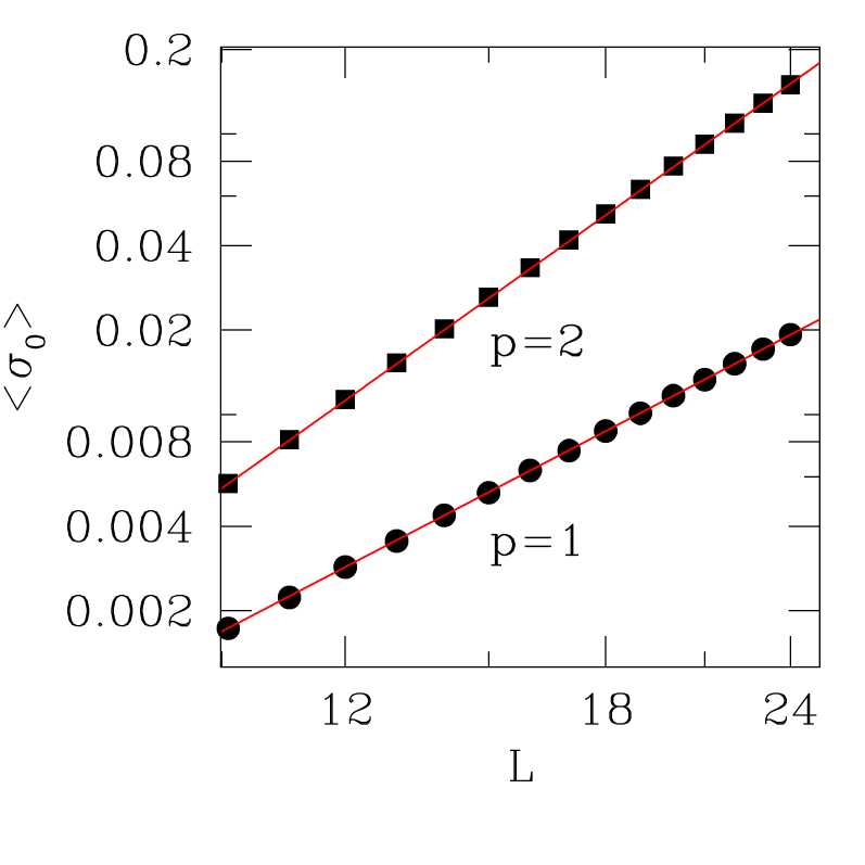
Figure 1: (Color online) Double-logarithmic plot of magnetizations at strip center for $p=1$ and $p=2$, against strip width $L$. Here, $h_{0}=10^{-5}$. The straight lines are guides to the eye, with respective slopes $2.75$ ($p=1$) and $3.75$ ($p=2$); see Eq. (7).

Furthermore, one can test the amplitude ratio ${\cal A}(p_{1})/{\cal A}(p_{2})$, by plotting $\langle\sigma_{0}(p_{1},L)\rangle/\langle\sigma_{0}(p_{2},L)\rangle$ against $L^{p_{1}-p_{2}}$. Our results for $p_{1}=1$, $p_{2}=2$ are shown in Fig. 2. TM data are well-adjusted by a linear least-squares fit ($y=ax+b$) with $b=0.001(1)$, providing complementary evidence in favor of the single power-law scenario of Eq. (7). The adjusted slope is $a=3.01(2)$, to be compared to the predictions of Eqs. (9) and (10), ${\cal A}(1)/{\cal A}(2)=2.98(1)$, where the uncertainty follows from allowing $\alpha$ of Eq. (10) to vary between $1.0$ and $1.5$.

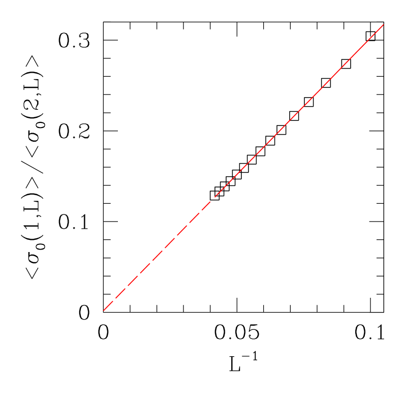
Figure 2: (Color online) Plot of the ratio of magnetizations on the trapping axis, $\langle\sigma_{0}(p_{1},L)\rangle/\langle\sigma_{0}(p_{2},L)\rangle$ against $L^{p_{1}-p_{2}}$ for $10\leq L\leq 24$, $p_{1}=1$, $p_{2}=2$, with $h_{0}=10^{-5}$. Points are TM results; the line is a linear least-squares fit of data (see text).

We conclude that the linear response approach, in conjunction with conformal invariance concepts, is a suitable description of the low-field magnetization properties of the trapping problem on a strip geometry.

Our next step is to investigate the magnetization profiles across the system. If the origin of coordinates in the integrals is now set at a distance $y_{1}$ from the trapping axis, $0<y_{1}\leq L/2$, and defining the reduced coordinate $u\equiv y_{1}/L$, one can see that the long-distance contribution $A_{1}(u,p)$ to ${\cal A}(u,p)$ [$\equiv{\cal A}(u)$, for short] is still given by Eq. (9). The short-distance part $A_{2}(u)$ can no longer be analytically expressed in a relatively simple form, because the symmetries used in establishing Eq. (10) no longer hold off-axis. However, one can still evaluate the corresponding integrals numerically, in which case the full form of Eq. (6) can be used over the whole domain of integration. We have found that, in general:

(i) the order of magnitude of $A_{2}(u)$ remains similar to that of $A_{1}$, as is the case on the strip axis [see Eqs. (9) and  (10)];

(ii) the fractional variation $({\cal A}(1/2)-{\cal A}(0))/{\cal A}(0))$ from axis to edge increases with $p$, from $\approx 2.5\%$ for $p=1$ to $\approx 6\%$ for $p=8$;

(iii) as suggested by Eq. (7), together with generic scaling ideas, one gets good scaling plots of TM results, $L^{-(p+2-\eta)}\,\langle\sigma_{y_{1}}\rangle$, against $u$.

We first illustrate the suitability of the linear-response plus conformal-invariance approach, in the description of numerical TM data for magnetization profiles. Figure 3 shows scaled magnetization data for $p=1$, $L=24$, as well as ${\cal A}(u)$ calculated by numerical integration.

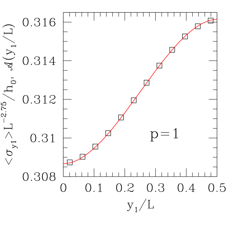
Figure 3: (Color online) Scaled magnetization TM data, $h_{0}^{-1}\,L^{-(p+2-\eta)}\langle\sigma_{y_{1}}\rangle$, for $L=24$ (points), together with the result of linear response plus conformal-invariance approach (solid line). Both for $p=1$. The horizontal axis is $u=y_{1}/L$.

Apart from an overall normalization factor for ${\cal A}$, which affects only the vertical scale, there are no fitting parameters. One sees that the agreement is very good.

As regards point (ii), Fig. 4 provides a visual comparison of calculated profiles ${\cal A}(u)$ for $p=1$, $2$, and $8$, together with TM results for $p=1$ and $2$ (the latter, both for $L=24$). In order to exhibit fractional variations more clearly, all curves have been normalized to unity at $u=0$. Note that, for $p=2$, the agreement between TM data and the respective calculated profile is as good as that for $p=1$. TM calculations for the low-field regime $L/\ell\ll 1$ with $p=8$ have proved rather unwieldy, as the corresponding fields on strip sites become numerically extremely small, thus we do not present a comparison between the calculated profile and TM data for this case. In this connection, one must recall that the physically more interesting trap shapes correspond to $p=1$ and $2$, since $p$ large approaches an infinite well.

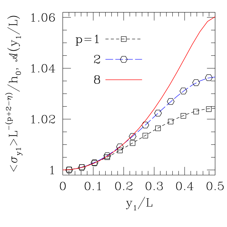
Figure 4: (Color online) Calculated profiles ${\cal A}(u)$ for $p=1$, $2$, and $8$. Points are scaled magnetization TM data, $h_{0}^{-1}\,L^{-(p+2-\eta)}\langle\sigma_{y_{1}}\rangle$, for $p=1$ and $2$, both for $L=24$. The horizontal axis is $u=y_{1}/L$. All curves have been normalized to unity at $u=0$.

For the data collapse mentioned in point (iii), we found that strong even-odd oscillations are present, thus in the following we restrict ourselves to even lattice widths. We also consider only $p=1$, which gives the smoothest results, as expected from the fact that this setup corresponds to a shallow trap shape. Finally, corrections to scaling are present which are small but noticeable for small and intermediate strip widths. These have been accounted for in the usual way dq09 , by assuming

$$h_{0}^{-1}\,L^{-(p+2-\eta)}\,\langle\sigma_{y_{1}}\rangle=f_{p}(y_{1}/L)+L^{-\omega}\,g_{p}(y_{1}/L)\ .$$ (13)

Here, $\omega>0$ is the exponent associated to the leading irrelevant operator. We found that, with $\omega=1$, and $g_{1}(y_{1}/L)=c$ (constant), the best data collapse is obtained for $c=-7.0(2)\times 10^{-5}$. This is shown in Fig. 5.

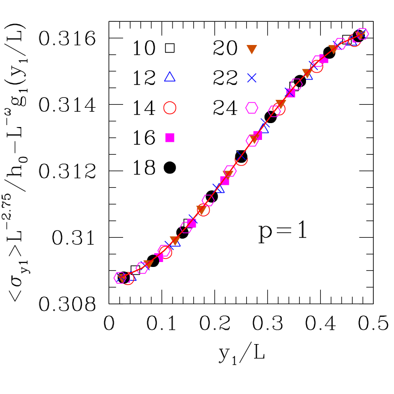
Figure 5: (Color online) $p=1$: data collapse for scaled magnetization TM results, including corrections to scaling, i.e., $h_{0}^{-1}\,L^{-2.75}\langle\sigma_{y_{1}}\rangle-L^{-\omega}g_{1}(y_{1}/L)$ [see Eq. (13)], for $10\leq L\leq 24$ (even widths only). The horizontal axis is $u=y_{1}/L$.

IV High-field regime

In order to make contact with previous work cv09 , we have set $p=2$, and generated data for strips with varying $L$ and $\ell$, initially keeping constant the ratio $\ell/L=1/\sqrt{2}$.

The average energy per site $e_{s}$ can be calculated, for a system with nearest-neighbor interactions on a square-lattice geometry, as $e_{s}=e_{x}+e_{y}$, where $e_{x}$, $e_{y}$ are the energies of the bonds along each coordinate axis. On a strip of width $L$ sites with PBC across, with the TM advancing along $x$, one finds for the Ising spin-$1/2$ model at $T_{c}$ and in the absence of (trapping or uniform) field, that $e_{x,y}=e_{b}^{0}+a_{x,y}\,L^{-2}+b_{x,y}\,L^{-4}+{\cal O}(L^{-6})$. Sequences of $e_{x}$, $e_{y}$ generated using $4\leq L\leq 16$ give $a_{y}/a_{x}=b_{y}/b_{x}=-1$ to four significant digits ($a_{y},b_{y}>0$). Both extrapolate to the exact value $e_{b}^{0}=\sqrt{2}/2$ to four significant digits, while the average between the two extrapolates agrees with that to six digits.

Upon inclusion of the trapping field as described above, its value at sites near the strip edge becomes rather large. The site energies now vary with position across the strip. Since signatures of a scaling regime should be more apparent where deviatons of the relevant fields from their critical values are small, at least in a local sense, we calculate energies for the sites at, or nearest to, the strip center. A similar reasoning appears to have been followed in the Monte Carlo simulations of Ref. cv09, .

The resulting sequences of $e_{x}$ and $e_{y}$ exhibit even-odd oscillations. However, these are smoothed out when $e_{s}$ is considered instead. Fitting data for $10\leq L\leq 23$ to $e_{s}=\sqrt{2}+a\,\ell^{-\theta}\,(1+b\,\ell^{-2})$ gives $\theta=0.514(10)$, in very good agreement with the scaling prediction cv09 , $\theta=16/31=0.51613\dots$ .

Next, we consider local magnetizations $m_{0}$, again on sites at, or nearest to, the strip center, for the same reasons invoked above in regard to site energies. The magnetization sequences show significant even-odd oscillations, thus we ran separate fits for data subsets corresponding to even and odd $L$. Using $10\leq L\leq 23$, assuming $m_{0}=c\,\ell^{-\phi}\,(1+d\,\ell^{-2})$ we get $\phi=0.0646(8)$ from an average between the final estimates for even- and odd- sequences. This is again in very good agreement with the respective scaling prediction cv09 , $\phi=2/31=0.0645\dots$ .

In analogy with Eq. (4), and considering the uniform field $H\equiv 0$ from the start, the correlation length on a strip is given by:

$$\xi_{L}(t,\ell)=L\,f(Lt,L\,\ell^{-\theta})$$ (14)

At $t=0$, and applying standard FSS ideas, one expects:

$$\frac{L}{\pi\,\xi(0,\ell)}=g\left(\frac{L}{\ell^{\theta}}\right)\ ,\ \ g(x)\sim\begin{cases}{{\rm const.}\quad x\ll 1}\cr{x\qquad\quad x\gg 1}\end{cases}\ .$$ (15)

We generated correlation-length data for $4\leq L\leq 24$ and assorted $6\lesssim\ell\lesssim 20$, thus allowing $L/\ell$ to vary over a relatively broad extent. Recalling from conformal-invariance cardy that $L/\pi\,\xi_{L}(0,0)=\eta=1/4$, we plotted $L/\pi\,\xi_{L}(0,\ell)$ against $L\,\ell^{-\theta}$ for tentative values of $\theta$, searching for the best data collapse. This was found along a somewhat broad range, $0.49\lesssim\theta\lesssim 0.52$, which includes both the trap-size scaling prediction and the mean-field value $\theta_{\rm MF}=1/2$. Fig. 6 shows a typical result, using $\theta=0.51$. The trends predicted in Eq. (15) are all verified.

Figure 6: (Color online) Scaled correlation-length data for $p=2$, with varying $L/\ell$ [see Eq. (15)]. The horizontal axis is $x\equiv L/\ell^{\theta}$, with $\theta=0.51$. The straight line through the origin is a guide to the eye.

In order to narrow down our error estimates, we investigated how well the large-$x$ portion of the data falls on a straight line, as predicted in Eq. (15). We fitted portions of data contained within intervals $x_{1}<x<x_{2}$ to a single power law with an adjustable exponent, $\varepsilon$. For $[x_{1},x_{2}]=[4,9]$, i.e. essentially all the large-$x$ region, we found $\varepsilon=1$ within $0.5\%$ for $\theta=0.503(7)$, while if we restricted ourselves to $[x_{1},x_{2}]=[4,6]$ the corresponding range of $\theta$ turned out to be $\theta=0.514(10)$.

Since the largest values of $x$ correspond to large $\ell^{-1}$, the respective correlation-length data belong to a region in parameter space away from the critical point, where the scaling behavior crosses over to a mean-field picture. Accordingly, when one includes such data in the analysis, the results for $\theta$ are biased towards its mean-field value; on the other hand, their exclusion brings the estimate of $\theta$ back towards the scaling prediction.

An analytic treatment of the correlation length can be given for the limit $p\to\infty$, providing for this case the scaling function $g(x)$ in Eq. (15), and having similarities to the form shown for $p=2$ in Figure 6. The reduction for $p\to\infty$ comes because the trapping well is there equivalent to confinement between $-\ell$ and $+\ell$, so strip geometry and well are together equivalent to a strip of width $L^{\prime}={\rm min}(L,2\ell)$. For this equivalent system, Eq. (6) (with $L$ replaced by $L^{\prime}$) can be used to obtain the effective correlation length, yielding for $p\to\infty$,

$$\frac{L}{\pi\,\xi_{L}(0,\ell)}=g\left(\frac{L}{\ell^{\theta}}\right)\ ,\ {\rm with}\ g(x)=\frac{\eta}{2}\,{\rm max}(2,x)\$$ (16)

[using $\theta(p=\infty)=1$, from Eq. (3)].

V Universality: Ising $S=1$ and Blume-Capel model

In this section, we investigate the universality of trapping scaling against varying features of the spin Hamiltonian. We shall keep $p=2$ in what follows. For TM calculations, the field setup is the same as defined in Sec. II, with the trapping axis halfway along the strip width.

We start by applying the ideas discussed in the previous Section to an Ising $S=1$ system, on a square lattice with nearest-neighbor couplings, in units of which the zero-field critical temperature is $T_{c}=1.69356(2)$ bcg03 . With the trapping field coupled to the magnetization, we considered the high-field regime, making again $\ell=L/\sqrt{2}$ as our starting point.

At the zero-field critical point, by considering the bond energies $e_{x}$ and $e_{y}$ as in Sec. IV, we found from fits of data for $4\leq L\leq 13$ that $e_{s}^{0}=1.16100(2)$, to be compared with $e_{s}^{0}=1.16094(5)$ bn85 . Upon introducing the trapping field, we restricted ourselves to the sites closest to the strip center, for the reasons invoked in Sec. IV. Fitting data for $4\leq L\leq 15$ (even- and odd-$L$ sequences have to be considered separately, on account of the associated oscillations) to $e_{s}=e_{s}^{0}+a_{1}\ell^{-\theta}(1+b_{1}\ell^{-2})$ gives $\theta=0.55(2)$, where the error bar reflects the spread among fits of differing subsets of data: odd/even, and vertical/horizontal/vertical-plus-horizontal bond energies.

For the local magnetization closest to the strip center, for $4\leq L\leq 15$ we again resorted to separate fits for even- and odd-$L$ sequences. The relative shortness of such sequences, compared to the $S=1/2$ case, makes extrapolation somewhat risky. However, by attempting power-law fits $m_{0}=c_{1}\ell^{-\phi}(1+d_{1}\ell^{-2})$, we saw that, by successively excluding an increasing number of smaller strips widths, the sequences of estimates for $\phi$ vary as: $\phi=0.088(4)$, $0.075(2)$, $0.070$ ($L$ even); and $\phi=0.099(6)$, $0.078(2)$, $0.071(2)$, $0.068$ ($L$ odd). Thus, it seems plausible that consideration of larger $L$ would produce a result compatible with the prediction $\phi=2/31$ cv09 .

Next, by allowing the trapping field intensity (thus, the corresponding length $\ell$) to vary independently of $L$, we extracted an independent estimate of $\theta$ via the scaling argument presented in Eqs. (14) and (15). We used $4\leq L\leq 15$, and $2\lesssim\ell\lesssim 9$. For tentative values of $\theta$ close to $0.5$, we found a scaling curve quantitatively very similar to that for $S=1/2$, shown in Fig. 6. Indeed, the respective numerical values stay within at most $3-4\%$ from those of the $S=1/2$ curve. However, the quality of data collapse is markedly inferior; furthermore, it does not appear possible to have good scaling with a single $\theta$ for the whole curve. For $\theta=0.47$, points fall very well on a straight line at large $x=L/\ell^{\theta}$, while those at smaller $x$ show a somewhat large degree of scatter. For $\theta=1/2$ the situation is reversed.

Overall, the above results are in fair agreement with the hypothesis of universal behavior against spin value, though with some degree of scatter. Note that the estimates for $\theta$ from internal-energy and correlation-length scaling are, respectively, above and below the expected value $\theta=16/31$; thus, we have found no systematic trend away from universality.

We now turn to discussing the application of a trapping field to a variant of the $S=1$ Ising model, namely the Blume-Capel (BC) model b66 ; c66 ; beale ; xapp98 ; dgb05 , on a two-dimensional square lattice. The Hamiltonian is:

$${\cal H}=-J\sum_{(i,j)}S_{i}S_{j}+\left(D+h_{0}\,|{\vec{r}}_{i}|^{p}\right)\sum_{i}S_{i}^{2}\ ,$$ (17)

where $S_{i}=\pm 1,0$ (spin–$1$ Ising variables). With $J>0$ (taken to be unity from now on) and $D,h_{0}>0$, the field term privileges vacancies, so there is an immediate mapping between $\langle S^{2}\rangle$ and the "particle" density in the lattice-gas picture. The BC model was studied recently via Monte Carlo simulations, in a trapping field with $p=1$, and assorted values of $D$ pbs08 .

Considering for now $h_{0}=0$, it is known that for $D>0$ the competition between field and spin-spin coupling leads to a tricritical point at $T_{t}=0.6085776(1)$, $D_{t}=1.9658149(2)$ beale ; xapp98 ; dgb05 . For $D<D_{t}$ the behavior along the $D-T$ critical line is governed by the Ising spin–$1/2$ fixed point at $D\to-\infty$ (at which vacancies are effectively forbidden) xapp98 ; dgb05 .

Therefore, as regards the respective universality class of the (suppressed) phase transition, by fixing $D<D_{t}$ and taking $h_{0}\neq 0$ one is in fact crossing the critical line far away from its governing fixed point. Though this does not invalidate the conclusions of Ref. pbs08, , which concern the validity of the local-density approximation for calculating the internal energy and linear structure factor, one must expect strong crossover effects if attempting to evaluate critical indices there.

In what follows, we kept $D=0$, and $p=2$ in Eq. (17).

The "order parameter" associated to the trapping transition, i.e. the vacancy concentration, can be extrapolated from TM data for $4\leq L\leq 13$ to be $1-\langle S^{2}\rangle=0.16120(1)$, in excellent agreement with the estimate from Table IV of Ref. dgb05, , namely $\rho({\rm Ising})=0.1610(5)$. This is a reminder that one is working away from the critical point. Thus, for instance, in this case it is not possible to define the analogue of the magnetization exponent $\phi$ of Sec IV.

On the other hand, since for sufficiently small $h_{0}$ the associated length $\ell$ still diverges, at $t=0$ one can examine the interplay between $\ell$ and, say, $\xi_{L}(0,\ell)$, and find the respective scaling behavior and (apparent) exponents. With this proviso, the arguments leading to Eq. (15) are still valid. Using $4\leq L\leq 15$, and $2\lesssim\ell\lesssim 9$, we attempted data collapse of $L/\pi\xi_{L}(0,\ell)$ against $L/\ell^{\theta_{\rm app}}$, with the best superposition for $\theta_{\rm app}=0.700(5)$. The results are shown in Fig. 7. Comparison of the respective numerical values shows that this scaling curve exhibits no superposition (except for the limiting constant value of $1/4$ at $x\to 0$) with that for the $S=1/2$ Ising case, shown in Fig. 6.

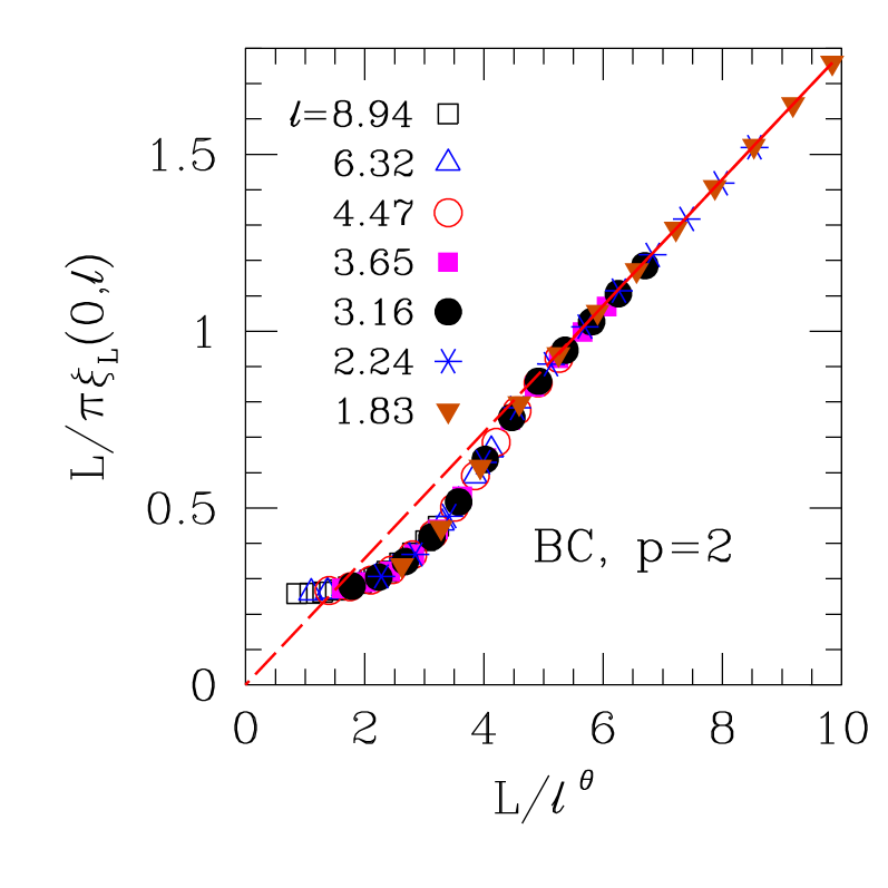
Figure 7: (Color online) Scaled correlation-length data for BC model, $p=2$, with varying $L/\ell$ [see Eq. (15)]. The horizontal axis is $x\equiv L/\ell^{\theta_{\rm app}}$, with $\theta_{\rm app}=0.700$. The straight line through the origin is a guide to the eye.

In a similar vein, we investigated the site energies. Making now $\ell/L=1/\sqrt{2}$, adjusting a sequence of data for $4\leq L\leq 15$ to $e_{s}=e_{s}^{0}+a^{\prime}\ell^{\,\theta_{\rm app}^{\prime}}$, we get $0.10\lesssim\theta_{\rm app}^{\prime}\lesssim 0.13$. The discrepancy between $\theta_{\rm app}^{\prime}$ and $\theta_{\rm app}$ of the correlation-length scaling again reflects the fact that one is not close to an actual fixed point.

VI Discussion and Conclusions

Thermodynamic systems with degrees of freedom subject to a trapping field bring yet another length scale into play, namely, that of the trap size, $\ell$. The latter is a measure of how far from the center the trapping field reaches a given intensity, $h_{0}=\ell^{-p}$, with $p$ describing the steepness; $p=2$ for the usual harmonic traps. Therefore, analyses of data extracted from systems of finite extent, $L$, (at least in one of its $d$ dimensions), must incorporate the interplay between these two independent length scales. We have proposed an extension of the usual finite-size scaling theory to deal with these problems, and tested it on classical (Ising) systems, for which the scaling limit of large $L$ can be easily achieved. The tests have been carried out on long strips of finite width $L$, subject to a trapping field translationally invariant along the "infinite" direction; the strip topology was that of a square lattice.

For all field regimes considered, the characteristic exponents of trap scaling vary continuously with $p$. This is analogous to what happens in the two-dimensional $XY$ model, which has a line of fixed points, and exponents varying along the line nelson . There, the position on the line is related to a relevant variable which is marginal in the sense that it does not remove criticality, although it does affect exponents. Here we have the same scenario (but without, yet, a flow diagram to support it).

In the low-field regime (i.e., for "shallow" traps, $\ell\gg L$) one expects a linear-response scenario to be appropriate. For Ising systems we can therefore use this, together with exact conformal-invariance results, to produce analytical predictions to be compared with numerical results from TM methods, at the critical point of the otherwise infinite and untrapped system. We have established that, in accordance with our ansatz, the local magnetization displays the scaling behavior

$$\langle\sigma_{y_{1}}\rangle=h_{0}\,L^{(p+2-\eta)}\,f_{p}(y_{1}/L),$$ (18)

to leading order in $h_{0}$, where $y_{1}$ is the distance from the center along the finite strip direction; see Sec. III.

In the high-field regime, $\ell\lesssim L$, scaling bears the signature of the $p$-dependent trap exponent $\theta$, as previously discussed in Ref. cv09, [see Eq. (3)]. For $p=2$ we have provided independent checks of the exponents for the scaling at criticality of the central magnetization and of the energy density, in very good numerical agreement with Ref. cv09, . Furthermore, with our TM calculations over a broad range of values of $\ell$ and $L$ (spin-1/2), we have established that the scaled correlation lengths behave as $L/\pi\,\xi_{L}(\ell)\sim g(L/\ell^{\theta})$, where the function $g(x)$ very accurately follows a form predicted by scaling arguments. Controlling for the quality of data collapse provides us with an estimate for the exponent $\theta\approx 0.51$ (for $p=2$) which agrees very well with the respective scaling prediction, $\theta=16/31$. We have also given an analytic treatment which describes how the finite-$p$ scaling function evolves, in the $p\to\infty$ limit, towards a piecewise straight-line shape [see Eq. (16)].

As a further check of the theory, we have also considered the high-field regime for a spin-1 Ising model in two situations. The first corresponds to an immediate extension of the spin-1/2 case, in which the trapping field couples to the magnetization. Since the TMs for $S=1$ are larger than for $S=1/2$, we were not able to consider linear lattice sizes as large as previously. Thus, the quality of the data collapse and scaling fits was somewhat compromised; however, our results are broadly consistent with fits to the same exponents as before, namely, $\theta=16/31$ and $\phi=\theta\beta/\nu=2/31$ (in standard notation of critical exponents) for $p=2$. This picture therefore gives support to the universality of trapping exponents against spin magnitude.

We have also examined the Blume-Capel (BC) model, with the trapping field coupling to $\sum_{i}S_{i}^{2}$ (whose average gives the "particle density", in the lattice-gas language). This latter feature might be considered a more transparent way to connect the spin language to that of particle trapping. However, we have seen that the fixed-point structure of the BC phase diagram puts one at a disadvantage, concerning the estimation of scaling exponents for physically plausible values of the model’s parameters. Notwithstanding this, we have been able to show that the competition between the associated scaling fields, $L^{-1}$ and $\ell^{-1}$, gives rise to an effective scaling picture in qualitative agreement with standard FSS ideas.

- (1) E. A. Cornell and C. E. Wieman, Rev. Mod. Phys. 74, 875 (2002).
- (2) W. Ketterle, Rev. Mod. Phys. 74, 1131 (2002).
- (3) U. Schneider, L. Hackermüller, S. Will, Th. Best, I. Bloch, T. A. Costi, R. W. Helmes, D. Rasch, and A. Rosch, Science 322, 1520 (2008).
- (4) I. Bloch, J. Dalibard, and W. Zwerger, Rev. Mod. Phys. 80, 885 (2008).
- (5) M. Köhl, Phys. Rev. A73, 031601(R) (2006).
- (6) W. Ketterle, Y. Shin, A. Schirotzek and C. H. Schunk, J. Phys.: Condens. Matter 21, 164206 (2009).
- (7) M. N. Barber, in Phase Transitions and Critical Phenomena, edited by C. Domb and J. L. Lebowitz (Academic, New York, 1983), Vol. 8.
- (8) M. Campostrini and E. Vicari, Phys. Rev. Lett. 102, 240601 (2009).
- (9) such effects have been considered in M. Campostrini and E. Vicari, e-print arXiv:0906.2640.
- (10) S. M. Pittman, G. G. Batrouni, and R. T. Scalettar, Phys. Rev. B78, 214208 (2008).
- (11) M. P. Nightingale, in Finite Size Scaling and Numerical Simulations of Statistical Systems, edited by V. Privman (World Scientific, Singapore, 1990).
- (12) S. Wessel, F. Alet, M. Troyer, and G. G. Batrouni, Phys. Rev. A70, 053615 (2004).
- (13) J. L. Cardy, in Phase Transitions and Critical Phenomena, edited by C. Domb and J. L. Lebowitz (Academic, New York, 1987), Vol. 11.
- (14) S. L. A. de Queiroz and R. B. Stinchcombe, Phys. Rev. B68, 144414 (2003).
- (15) S. L. A. de Queiroz, Phys. Rev. B73, 064410 (2006).
- (16) see, e.g., S. L. A. de Queiroz, Phys. Rev. B79, 174408 (2009) and references therein.
- (17) P. Butera, M. Comi, and A. J. Guttmann, Phys. Rev. B67, 054402 (2003).
- (18) H. W. J. Blöte and M. P. Nightingale, Physica A 134, 274 (1985).
- (19) M. Blume, Phys. Rev. 141, 517 (1966).
- (20) H. W. Capel, Physica (Amsterdam) 32, 966 (1966).
- (21) P. D. Beale, Phys. Rev. B33, 1717 (1986).
- (22) J. C. Xavier, F. C. Alcaraz, D. Pena Lara, and J. A. Plascak, Phys. Rev. B57, 11575 (1998).
- (23) Y. Deng, W. Guo, and H. W. J. Blöte, Phys. Rev. E72, 016101 (2005).
- (24) D. R. Nelson, in Phase Transitions and Critical Phenomena, edited by C. Domb and J. L. Lebowitz (Academic, New York, 1983), Vol. 7.