FR-PHENO-2010-15

PSI-PR-10-06

ZU-TH 04/10

Electroweak corrections to hadronic event shapes
and jet production in $\mathrm{e}^{+}\mathrm{e}^{-}$ annihilation
Ansgar Denner^a, Stefan Dittmaier^b, Thomas Gehrmann^c, Christian Kurz^a,c
a Paul Scherrer Institut, CH-5232 Villigen PSI, Switzerland
^b Physikalisches Institut, Albert-Ludwigs-Universität Freiburg, D-79104 Freiburg, Germany
^c Institut für Theoretische Physik, Universität Zürich, CH-8057 Zürich, Switzerland

We present a complete calculation of the electroweak ${\cal O}(\alpha^{3}\alpha_{\mathrm{s}})$ corrections to three-jet production and related event-shape observables at electron–positron colliders. The Z-boson resonance is described within the complex-mass scheme, rendering the calculation valid both in the resonance and off-shell regions. Higher-order initial-state radiation is included in the leading-logarithmic approximation. We properly account for the corrections to the total hadronic cross section and for the experimental photon isolation criteria. To this end we implement contributions of the quark-to-photon fragmentation function both in the slicing and subtraction formalism. The effects of the electroweak corrections on various event-shape distributions and on the three-jet rate are studied. They are typically at the few-per-cent level, and remnants of the radiative return are found even after inclusion of appropriate cuts.

March 2010

1 Introduction

Jet production in $\mathrm{e}^{+}\mathrm{e}^{-}$ annihilation provides an ideal environment for studies of the dynamics of the strong interaction, described by the theory of quantum chromodynamics (QCD) [1]. The kinematical distribution of jets closely reflects the parton-level kinematics of the event. Consequently, the first observation of three-jet final states at DESY PETRA [2], produced through quark–antiquark–gluon final states [3], provided conclusive evidence for the existence of the gluon. Jets are defined through a jet algorithm, which is a procedure to recombine individual hadrons into jets using a distance measure, resolution criterion and recombination prescription. The theoretical description applies the same jet algorithm to partons in the final state. Closely related to jet cross sections are event-shape distributions. Event-shape variables measure certain geometrical properties of hadronic final states, and can equally be calculated in perturbative QCD from partonic final states.

Jet cross sections and event-shape distributions were studied very extensively at $\mathrm{e}^{+}\mathrm{e}^{-}$ colliders [4], and high-precision data are available from the LEP experiments ALEPH [5], OPAL [6], L3 [7], DELPHI [8], from SLD [9] at SLAC and from JADE [10] at DESY PETRA. The theoretical description of these data in perturbative QCD contains only a single parameter: the strong coupling constant $\alpha_{\mathrm{s}}$. By comparing experimental results with the theoretical description, one can thus perform a measurement of $\alpha_{\mathrm{s}}$ from jet cross sections and event shapes. For a long period, the perturbative description of these observables was based on next-to-leading order (NLO) [11, 12, 13] in perturbative QCD, improved by the resummation of next-to-leading-logarithmic corrections [14] to all orders. The uncertainty on these theoretical predictions from missing higher-order terms results in a theory error on the extraction of $\alpha_{\mathrm{s}}$, which was quantified to be around five per cent, and thus larger than any source of experimental uncertainty.

Owing to recent calculational progress, the QCD predictions for event shapes [15, 16] and three-jet production [17, 18] are now accurate to next-to-next-to-leading order (NNLO, $\alpha^{2}\alpha_{\mathrm{s}}^{3}$) in QCD perturbation theory. Inclusion of these corrections results in an estimated residual uncertainty of the QCD prediction from missing higher orders at the level of well below five per cent for the event-shape distributions, and around one per cent for the three-jet cross section. Using these results (combined [19] with the previously available resummed expressions), new determinations of $\alpha_{\mathrm{s}}$ from event-shape and jet production data were performed, resulting in a considerable improvement of the theory uncertainty to three per cent from event shapes [20] and below two per cent from jet rates [21]. A further improvement can be anticipated for the event shapes from the resummation of subleading logarithmic corrections [22].

At this level of theoretical precision, higher-order electroweak effects could be of comparable magnitude. Until recently, only partial calculations of electroweak corrections to three-jet production and event shapes have been available [23], which can not be compared with experimental data directly. In a previous work [24], we briefly reported our results on the first calculation of the NLO electroweak ($\alpha^{3}\alpha_{\mathrm{s}}$) corrections to three-jet observables in $\mathrm{e}^{+}\mathrm{e}^{-}$ collisions including the quark–antiquark–photon ($q\bar{q}\gamma$) final states. Here, we describe this calculation in detail and perform extensive numerical studies on the impact of the electroweak corrections to three-jet-like observables at different $\mathrm{e}^{+}\mathrm{e}^{-}$ collider energies.

The full NLO electroweak ($\alpha^{3}\alpha_{\mathrm{s}}$) corrections to jet observables contain four types of contributions: genuine weak corrections from virtual exchanges, photonic corrections to quark–antiquark–gluon ($q\bar{q}g$) final states, gluonic corrections to $q\bar{q}\gamma$ final states, and QCD/electroweak interference effects in $q\bar{q}q\bar{q}$ final states of identical quark flavour. The latter were not included in our previous work, but turn out to be numerically negligible as anticipated.

Any jet-like observable at NLO in the electroweak theory receives virtual one-loop corrections and contributions from real photon radiation. Experimental cuts on isolated hard photons in the final state allow to suppress these real photon contributions. However, photons radiated inside hadronic jets can often not be distinguished from hadrons (like neutral pions), and are thus not removed by experimental cuts. The real photon contribution at NLO thus results from a complicated interplay of jet reconstruction and photon isolation cuts. Through the isolated-photon veto, these observables are sensitive to final-state particle identification, and thus to fragmentation processes. In our case, we must include a contribution from quark-to-photon fragmentation [25] to obtain a well-defined and infrared-safe observable. Since our calculation is among the very first to perform electroweak corrections to jet observables with realistic photon isolation cuts, we describe the relevant calculational aspects in detail below.

To define the observables considered here, we describe in Section 2 the jet-clustering algorithms used in $\mathrm{e}^{+}\mathrm{e}^{-}$ annihilation and the standard set of event-shape variables. In this section, we also review the current description of these observables in perturbative QCD. The calculation of NLO electroweak corrections is outlined in Section 3, where we describe the calculation of the virtual and real corrections in detail. The real corrections contain infrared divergences from unresolved photon and gluon radiation. These infrared divergences cancel against similar divergences in the virtual corrections. To accomplish this cancellation, it is, however, necessary to extract them analytically from the real corrections, which is done by a slicing or subtraction procedure (described in Section 4). Our results are implemented into a parton-level event generator (described in Section 5), which allows the simultaneous evaluation of all event-shape variables and jet cross sections. Numerical results for jet production and event-shape distributions for $\mathrm{e}^{+}\mathrm{e}^{-}$ collision energies at LEP1, LEP2 and a future linear collider are presented in Section 6. At energies above the $\mathrm{Z}$ peak, we observe non-trivial kinematical structures in the distributions. It is shown that these structures are a remnant of the radiative-return phenomenon, resulting from a complicated interplay of event-selection and photon isolation cuts applied in the experimental definition of the observables. Finally, we conclude with an outlook on the impact of electroweak effects on future precision QCD studies at $\mathrm{e}^{+}\mathrm{e}^{-}$ colliders in Section 7.

2 Jet observables

A commonly used method for reconstructing jets was originally introduced by the JADE group [26]. The algorithm is based on successive combinations. In a first step, each observed particle is listed as a jet. In the next step, a resolution parameter $y_{ij}$ is calculated for each particle pair, and the particle pair leading to the smallest value of $y_{ij}$ is combined into a single pseudo-particle. This yields a new list of jets, and the algorithm proceeds with step two. The procedure is repeated until no pair of particles is left with $y_{ij}<y_{\mathrm{cut}}$, where $y_{\mathrm{cut}}$ is a preset cut-off.

Different proposals exist in the literature in how to define $y_{ij}$ (see e.g. Ref. [27]). The original JADE definition reads

$$y_{ij,\mathrm{J}}=\frac{2E_{i}E_{j}\left(1-\cos\theta_{ij}\right)}{E_{\mathrm{vis}}^{2}},$$ (2.1)

where $E_{i}$ is the energy of the $i$-th particle, $\cos\theta_{ij}$ the angle between the particles, and $E_{\mathrm{vis}}$ the total visible hadronic energy in the event. Improving upon this definition, different jet resolution parameters have been proposed. Most widely used at LEP was the $k_{\mathrm{T}}$ or Durham algorithm [28, 29], which defines

$$y_{ij,\mathrm{D}}=\frac{2\min\left(E_{i}^{2},E_{j}^{2}\right)\left(1-\cos\theta_{ij}\right)}{E_{\mathrm{vis}}^{2}}\,.$$ (2.2)

In addition to the choice of jet resolution parameter, there also exist different ways of combining the four-momenta of the two particles with the lowest $y_{ij}$ to one four-momentum $p_{ij}$. In the so-called $E$-scheme one simply adds the two four-momenta, leading to $p_{ij}=p_{i}+p_{j}$. In the $P$-scheme the invariant mass of the pseudo-particle is set to zero by rescaling the energy

$${\vec{p}}_{ij}={\vec{p}}_{i}+{\vec{p}}_{j},\qquad E_{ij}=|{\vec{p}}_{i}+{\vec{p}}_{j}|.$$ (2.3)

In the $P_{0}$-scheme, (2.3) is used to construct the resulting four-momentum, however, after each recombination $E_{\mathrm{vis}}$ is recalculated. Finally, in the $E_{0}$-scheme the three-momentum rather than the energy is rescaled.

Since an event containing three jets is due to the emission of a gluon off an (anti-)quark at a large angle and with significant energy, the ratio of the number of observed three-jet to two-jet events is, in leading order, proportional to the strong coupling constant. In general, the $n$-jet rate $R_{n}(y)$, which depends on the choice of the jet resolution parameter $y=y_{\mathrm{cut}}$, is defined through the respective cross sections for $n\geq 2$ jets

$$R_{n}(y,\sqrt{s})=\frac{\sigma_{\mbox{\scriptsize$n$-jet}}}{\sigma_{\mathrm{had}}},$$ (2.4)

such that

$$\sum_{n=1}^{\infty}R_{n}(y)=1$$ (2.5)

and $\sqrt{s}$ is the centre-of-mass (CM) energy. In order to characterise the topology of an event a large number of observables have been developed. Most of them require at least three momenta of final-state particles to be non-trivial. In the following we introduce six variables which have been extensively used in experimental analyses: thrust $T$ [30, 31], the normalised heavy-jet mass $\rho$ [32], the wide and total jet broadenings $B_{\mathrm{W}}$ and $B_{\mathrm{T}}$ [33, 34], the $C$-parameter [35, 36], and the transition from three-jet to two-jet final-state using $y_{ij,\mathrm{D}}$ [29, 28, 37, 38].

• Thrust is defined through

  $$T=\max_{\vec{n}}\frac{\sum_{i}|\vec{p}_{i}\cdot\vec{n}|}{\sum_{i}|\vec{p}_{i}|},$$ (2.6)

  where $\vec{p}_{i}$ is the three-momentum of the $i$-th particle, and $\vec{n}$ is varied to maximise the momentum flow in its direction, yielding the thrust axis.

• Every event can be divided into two hemispheres $H_{1}$ and $H_{2}$ by a plane perpendicular to the thrust axis. In each hemisphere $H_{i}$ one can calculate the invariant mass $M_{i}^{2}$, the larger of which yields the heavy-jet mass

  $$M_{\mathrm{had}}^{2}=\max\left(M_{1}^{2},M_{2}^{2}\right),$$ (2.7)

  and the normalised heavy-jet mass

  $$\rho=\frac{M_{\mathrm{had}}^{2}}{E_{\mathrm{vis}}^{2}}.$$ (2.8)

• Using the definition of the hemispheres from above, one can calculate the hemisphere broadenings

  $$B_{i}=\frac{\sum_{j\in H_{i}}|\vec{p}_{j}\times\vec{n}|}{2\sum_{j}|\vec{p}_{j}|},\quad i=1,2.$$ (2.9)

  The wide and total jet broadenings $B_{\mathrm{W}}$ and $B_{\mathrm{T}}$ are then obtained through

  $$B_{\mathrm{W}}=\max\left(B_{1},B_{2}\right),\qquad B_{\mathrm{T}}=B_{1}+B_{2}.$$ (2.10)

• Starting from the linearised momentum tensor

  $$\Theta^{\alpha\beta}=\frac{1}{\sum_{i}|\vec{p}_{i}|}\sum_{j}\frac{p_{j}^{\alpha}p_{j}^{\beta}}{|\vec{p}_{j}|},\quad\alpha,\beta=1,2,3,$$ (2.11)

  and its three eigenvalues $\lambda_{1},\lambda_{2},\lambda_{3}$, the $C$-parameter is defined through

  $$C=3\left(\lambda_{1}\lambda_{2}+\lambda_{2}\lambda_{3}+\lambda_{3}\lambda_{1}\right).$$ (2.12)

• The jet transition variable $Y_{3}$ is defined as the value of the jet resolution parameter for which an event changes from a three-jet-like to a two-jet-like configuration.

In the following we often denote event-shape observables generically $y$. Taking $(1-T)$ instead of $T$ the two-particle configuration is located at $y=0$ for all the event-shape variables defined above.

2.1 Event shapes and jet rates in perturbation theory

At leading order (LO), $\mathcal{O}{\left(\alpha^{2}\alpha_{\mathrm{s}}\right)}$, the first process that occurs at tree level in $\mathrm{e}^{+}\mathrm{e}^{-}$ annihilation is gluon radiation off a quark or antiquark (see Fig. 1).

      

Figure 1: Lowest-order diagrams for $\mathrm{e}^{+}\mathrm{e}^{-}\rightarrow q\bar{q}\mathrm{g}$.

As mentioned above, by comparing the measured three-jet rate and event-shape observables with theoretical predictions, one can determine $\alpha_{\mathrm{s}}$.

In perturbation theory up to next-to-next-to-leading order (NNLO) in QCD, the expansion of a distribution in the generic observable $y$ at CM energy $\sqrt{s}$ for renormalisation scale $\mu=\sqrt{s}$ and $\alpha_{\mathrm{s}}=\alpha_{\mathrm{s}}(s)$, normalised to the Born cross section $\sigma_{0}(s)$ of the process $\mathrm{e}^{+}\mathrm{e}^{-}\rightarrow q\bar{q}$ is given by

$$\frac{1}{\sigma_{0}}\frac{{\mathrm{d}}\sigma}{{\mathrm{d}}y}=\left(\frac{\alpha_{\mathrm{s}}}{2\pi}\right)\frac{{\mathrm{d}}A}{{\mathrm{d}}y}+\left(\frac{\alpha_{\mathrm{s}}}{2\pi}\right)^{2}\frac{{\mathrm{d}}B}{{\mathrm{d}}y}+\left(\frac{\alpha_{\mathrm{s}}}{2\pi}\right)^{3}\frac{{\mathrm{d}}C}{{\mathrm{d}}y}+\mathcal{O}\left(\alpha_{\mathrm{s}}^{4}\right),$$ (2.13)

where $A$, $B$, and $C$ denote the QCD contributions of LO, next-to-leading order (NLO), and NNLO. The experimentally measured event-shape distribution is normalised to the total hadronic cross section $\sigma_{\mathrm{had}}$, which for massless quarks reads

$$\sigma_{\mathrm{had}}=\sigma_{0}\left(1+\left(\frac{\alpha_{\mathrm{s}}}{2\pi}\right)K_{1}+\left(\frac{\alpha_{\mathrm{s}}}{2\pi}\right)^{2}K_{2}+\mathcal{O}\left(\alpha_{\mathrm{s}}^{3}\right)\right),$$ (2.14)

such that

$$\frac{1}{\sigma_{\mathrm{had}}}\frac{{\mathrm{d}}\sigma}{{\mathrm{d}}y}=\left(\frac{\alpha_{\mathrm{s}}}{2\pi}\right)\frac{{\mathrm{d}}\bar{A}}{{\mathrm{d}}y}+\left(\frac{\alpha_{\mathrm{s}}}{2\pi}\right)^{2}\frac{{\mathrm{d}}\bar{B}}{{\mathrm{d}}y}+\left(\frac{\alpha_{\mathrm{s}}}{2\pi}\right)^{3}\frac{{\mathrm{d}}\bar{C}}{{\mathrm{d}}y}+\mathcal{O}\left(\alpha_{\mathrm{s}}^{4}\right),$$ (2.15)

where

$$\bar{A}=A,\qquad\bar{B}=B-AK_{1},\qquad\bar{C}=C-BK_{1}+AK_{1}^{2}-AK_{2}.$$ (2.16)

The coefficients in (2.16) up to NLO have been calculated in Refs. [11, 12, 13]. Furthermore, kinematically-dominant leading and next-to-leading logarithms have been resummed [39, 14], and non-perturbative models of power-suppressed hadronisation effects have been included [40, 41, 42, 43] to increase the theoretical accuracy. Recently the first NNLO calculations have been completed [15, 16, 17, 18], and the matching of next-to-leading logarithms and next-to-next-to-leading logarithms to the fixed-order NNLO calculation has been performed [22, 19]. These results have subsequently been used in precision determinations [20, 21, 22] of the strong coupling constant $\alpha_{\mathrm{s}}$.

With regard to jet rates, fixed-order calculations are known up to next-to-next-to-next-to-leading order ($\mathrm{N^{3}LO}$) in QCD for the two-jet rate [44, 45, 46, 17], up to NNLO for the three-jet rate [11, 12, 13, 17, 18], and up to NLO for the four-jet rate [47, 48, 49, 50, 51].

NLO electroweak (EW) corrections could be of comparable magnitude as the NNLO QCD corrections and are therefore worth further consideration. The factorisable EW corrections have been calculated in Ref. [52] and a further step towards the full NLO EW corrections has been made in Ref. [23]. In this work we describe the first calculation of the complete NLO EW corrections to the normalised event-shape distributions. First results of this calculation on the thrust distribution and the three-jet rate at $\sqrt{s}=M_{{\rm Z}}$ have been presented in Ref. [24].

In analogy to the QCD corrections, we write the total hadronic cross section including $\mathcal{O}{\left(\alpha\right)}$ corrections as

$$\sigma_{\mathrm{had}}=\sigma_{0}\left(1+\left(\frac{\alpha}{2\pi}\right)\delta_{\sigma,1}+\mathcal{O}\left(\alpha^{2}\right)\right),$$ (2.17)

and the expansion of the observable ${\mathrm{d}}\sigma/{\mathrm{d}}y$ as

$$\frac{1}{\sigma_{0}}\frac{{\mathrm{d}}\sigma}{{\mathrm{d}}y}=\left(\frac{\alpha_{\mathrm{s}}}{2\pi}\right)\frac{{\mathrm{d}}A}{{\mathrm{d}}y}+\left(\frac{\alpha}{2\pi}\right)\frac{{\mathrm{d}}\delta_{\gamma}}{{\mathrm{d}}y}+\left(\frac{\alpha}{2\pi}\right)\left(\frac{\alpha_{\mathrm{s}}}{2\pi}\right)\frac{{\mathrm{d}}\delta_{A}}{{\mathrm{d}}y}+\mathcal{O}\left(\alpha^{2}\right),$$ (2.18)

where the LO purely electromagnetic contribution $\delta_{\gamma}$ arises from tree-level quark–antiquark–photon ($q\bar{q}\gamma$) final states without a gluon and $\delta_{A}$ comprises the NLO EW corrections to the distribution ${\mathrm{d}}\sigma/{\mathrm{d}}y$.

Normalising (2.18) to $\sigma_{\mathrm{had}}$ yields

$$\frac{1}{\sigma_{\mathrm{had}}}\frac{{\mathrm{d}}\sigma}{{\mathrm{d}}y}=\left(\frac{\alpha_{\mathrm{s}}}{2\pi}\right)\frac{{\mathrm{d}}A}{{\mathrm{d}}y}+\left(\frac{\alpha}{2\pi}\right)\frac{{\mathrm{d}}\delta_{\gamma}}{{\mathrm{d}}y}+\left(\frac{\alpha}{2\pi}\right)\left(\frac{\alpha_{\mathrm{s}}}{2\pi}\right)\left(\frac{{\mathrm{d}}\delta_{A}}{{\mathrm{d}}y}-\frac{{\mathrm{d}}A}{{\mathrm{d}}y}\delta_{\sigma,1}\right)+\mathcal{O}\left(\alpha^{2}\right).$$ (2.19)

Hence, the full $\mathcal{O}{\left(\alpha\right)}$ EW corrections are given by

$$\frac{{\mathrm{d}}\delta_{\mathrm{EW}}}{{\mathrm{d}}y}=\left(\frac{\alpha}{2\pi}\right)\frac{{\mathrm{d}}\delta_{\gamma}}{{\mathrm{d}}y}+\left(\frac{\alpha}{2\pi}\right)\left(\frac{\alpha_{\mathrm{s}}}{2\pi}\right)\left(\frac{{\mathrm{d}}\delta_{A}}{{\mathrm{d}}y}-\frac{{\mathrm{d}}A}{{\mathrm{d}}y}\delta_{\sigma,1}\right).$$ (2.20)

In order to obtain a sensible ratio, all three contributions have to be evaluated using the same event-selection cuts.

The EW corrections to both $\sigma_{\mathrm{had}}$ and the distribution in $y$ contain large corrections due to initial-state radiation (ISR). Since these are universal, they partially cancel in the third term in (2.19), leaving only a small remainder. If we include higher-order leading-logarithmic (LL) ISR effects in both $\sigma_{\mathrm{had}}$ and the distribution in $y$, this leads to

$$\sigma_{\mathrm{had}}=\sigma_{0}\left(1+\left(\frac{\alpha}{2\pi}\right)\delta_{\sigma,1}+\left(\frac{\alpha}{2\pi}\right)^{2}\delta_{\sigma,\geq 2,\mathrm{LL}}+\mathcal{O}\left(\alpha^{2}\right)\right),$$ (2.21)

and

$$\frac{1}{\sigma_{0}}\frac{{\mathrm{d}}\sigma}{{\mathrm{d}}y}=\left(\frac{\alpha_{\mathrm{s}}}{2\pi}\right)\frac{{\mathrm{d}}A}{{\mathrm{d}}y}+\left(\frac{\alpha}{2\pi}\right)\frac{{\mathrm{d}}\delta_{\gamma}}{{\mathrm{d}}y}+\left(\frac{\alpha}{2\pi}\right)\left(\frac{\alpha_{\mathrm{s}}}{2\pi}\right)\frac{{\mathrm{d}}\delta_{A}}{{\mathrm{d}}y}+\left(\frac{\alpha}{2\pi}\right)^{2}\left(\frac{\alpha_{\mathrm{s}}}{2\pi}\right)\frac{{\mathrm{d}}\delta_{A,\geq 2,\mathrm{LL}}}{{\mathrm{d}}y}+\mathcal{O}\left(\alpha^{2}\right),$$ (2.22)

where $\delta_{\sigma,\geq 2,\mathrm{LL}}$ and $\delta_{A,\geq 2,\mathrm{LL}}$ contain leading-logarithmic (LL) terms proportional to $\alpha^{n}\ln^{n}({s}/{m_{\mathrm{e}}^{2}})$ with $n\geq 2$, as defined in Section 4.4. Here $\mathcal{O}\left(\alpha^{2}\right)$ stands for two-loop electroweak effects without the enhancement of leading ISR logarithms. For the normalised distribution this results in

$$\frac{1}{\sigma_{\mathrm{had}}}\frac{{\mathrm{d}}\sigma}{{\mathrm{d}}y} = \left(\frac{\alpha_{\mathrm{s}}}{2\pi}\right)\frac{{\mathrm{d}}A}{{\mathrm{d}}y}+\left(\frac{\alpha}{2\pi}\right)\frac{{\mathrm{d}}\delta_{\gamma}}{{\mathrm{d}}y}+\left(\frac{\alpha}{2\pi}\right)\left(\frac{\alpha_{\mathrm{s}}}{2\pi}\right)\left(\frac{{\mathrm{d}}\delta_{A}}{{\mathrm{d}}y}-\frac{{\mathrm{d}}A}{{\mathrm{d}}y}\delta_{\sigma,1}\right)$$

$${}+\left(\frac{\alpha}{2\pi}\right)^{2}\left(\frac{\alpha_{\mathrm{s}}}{2\pi}\right)\left[\left(\frac{{\mathrm{d}}\delta_{A,\geq 2,\mathrm{LL}}}{{\mathrm{d}}y}-\frac{{\mathrm{d}}A}{{\mathrm{d}}y}\delta_{\sigma,\geq 2,\mathrm{LL}}\right)-\frac{{\mathrm{d}}\delta_{A,1,\mathrm{LL}}}{{\mathrm{d}}y}\delta_{\sigma,1,\mathrm{LL}}+\frac{{\mathrm{d}}A}{{\mathrm{d}}y}\delta_{\sigma,1,\mathrm{LL}}^{2}\right]+\mathcal{O}\left(\alpha^{2}\right),$$

where $\delta_{A,1,\mathrm{LL}}$ and $\delta_{\sigma,1,\mathrm{LL}}$ denote the LL contributions contained in the NLO results. Their second-order effect results from taking the ratio of two NLO-corrected quantities. Therefore, the higher-order LL corrections read

$$\frac{{\mathrm{d}}\delta_{\mathrm{EW,LL}}}{{\mathrm{d}}y}=\left(\frac{\alpha}{2\pi}\right)^{2}\left(\frac{\alpha_{\mathrm{s}}}{2\pi}\right)\left[\left(\frac{{\mathrm{d}}\delta_{A,\geq 2,\mathrm{LL}}}{{\mathrm{d}}y}-\frac{{\mathrm{d}}A}{{\mathrm{d}}y}\delta_{\sigma,\geq 2,\mathrm{LL}}\right)+\left(\frac{{\mathrm{d}}A}{{\mathrm{d}}y}\delta_{\sigma,1,\mathrm{LL}}^{2}-\frac{{\mathrm{d}}\delta_{A,1,\mathrm{LL}}}{{\mathrm{d}}y}\delta_{\sigma,1,\mathrm{LL}}\right)\right].$$ (2.24)

Due to the universality of ISR, the terms in the first and in the second parenthesis in (2.24) separately cancel each other numerically to a large extent.

The same decomposition as applied here for event-shape distributions holds also for the three-jet rate, normalised to $\sigma_{\mathrm{had}}$.

2.2 Particle identification

One of the virtues of $\mathrm{e}^{+}\mathrm{e}^{-}$ colliders is the precise knowledge of the energy of the initial state. However, ISR of photons can lead to difficulties in the determination of the total energy of the final state. Therefore event-selection cuts have been devised to suppress effects due to ISR. In the following we describe the procedure employed by the ALEPH collaboration at LEP [53], which we use in our numerical evaluations.

First, particles are clustered into jets according to the Durham algorithm with $y_{\mathrm{cut,D}}=0.002$ and $E$-scheme recombination. Jets where the fraction of energy carried by charged hadrons is less than 10% are identified as dominantly electromagnetic and are removed. In the next step the remaining particles are clustered into two jets and the visible invariant mass $M_{\mathrm{vis}}$ of the two-jet system is calculated. Using total momentum conservation the reduced CM energy $\sqrt{s^{\prime}}$ is calculated. The event is rejected if $s^{\prime}/s<0.81$. This two-step procedure is later referred to as hard-photon cut procedure (note that it is called anti-ISR cut procedure in Ref. [53]).

Removing events where the photonic energy in a jet is higher than a certain value, as it is done in the hard-photon cuts, causes potential problems when perturbatively calculating EW corrections. There one relies on the cancellation of infrared (IR) singularities between virtual and real corrections when calculating an IR-safe observable. Removing events where a photon is close to a final-state charged fermion leads to non-IR-safe observables and spoils this cancellation in the collinear region. This feature is common to all observables with identified particles in the final state, and IR-finiteness is restored by taking into account a contribution from fragmentation processes, in our case from the quark-to-photon fragmentation function.

3 Structure of the calculation

To obtain the full EW ${\cal O}(\alpha^{3}\alpha_{\mathrm{s}})$ corrections to normalised event-shape distributions and jet cross sections we need to derive the NLO EW corrections to the total hadronic cross section and to the three-jet production cross section. The total hadronic cross section is decomposed as:

$$\sigma_{{\rm had}}=\int{\mathrm{d}}\sigma^{\mathrm{e}^{+}\mathrm{e}^{-}\rightarrow q\bar{q}}_{\mathrm{Born}}+\int{\mathrm{d}}\sigma^{\mathrm{e}^{+}\mathrm{e}^{-}\rightarrow q\bar{q}}_{\mathrm{virtual,EW}}+\int{\mathrm{d}}\sigma_{\mathrm{real}}^{\mathrm{e}^{+}\mathrm{e}^{-}\rightarrow q\bar{q}\gamma},$$ (3.1)

where the first and second terms are the Born and one-loop EW contributions to the process $\mathrm{e}^{+}\mathrm{e}^{-}\rightarrow q\overline{q}$, while the last term is the real radiation contribution from the process $\mathrm{e}^{+}\mathrm{e}^{-}\rightarrow q\overline{q}\gamma$. Likewise, we decompose the total cross section for three-jet production according to

$$\int{\mathrm{d}}\sigma = \int{\mathrm{d}}\sigma^{\mathrm{e}^{+}\mathrm{e}^{-}\rightarrow q\bar{q}g}_{\mathrm{Born}}+\int{\mathrm{d}}\sigma^{\mathrm{e}^{+}\mathrm{e}^{-}\rightarrow q\bar{q}\gamma}_{\mathrm{Born}}$$ (3.2)

$${}+\int{\mathrm{d}}\sigma^{\mathrm{e}^{+}\mathrm{e}^{-}\rightarrow q\bar{q}g}_{\mathrm{virtual,EW}}+\int{\mathrm{d}}\sigma^{\mathrm{e}^{+}\mathrm{e}^{-}\rightarrow q\bar{q}\gamma}_{\mathrm{virtual,QCD}}+\int{\mathrm{d}}\sigma_{\mathrm{real}}^{\mathrm{e}^{+}\mathrm{e}^{-}\rightarrow q\bar{q}g\gamma}+\int{\mathrm{d}}\sigma_{\mathrm{interference}}^{\mathrm{e}^{+}\mathrm{e}^{-}\rightarrow q\bar{q}q\bar{q}},$$

where the first and third terms are the Born and NLO EW contributions of the process $\mathrm{e}^{+}\mathrm{e}^{-}\rightarrow q\overline{q}g$, the second and fourth terms are the Born and one-loop QCD contributions of the process $\mathrm{e}^{+}\mathrm{e}^{-}\rightarrow q\overline{q}\gamma$, the fifth term is the contribution from the real radiation process $\mathrm{e}^{+}\mathrm{e}^{-}\rightarrow q\overline{q}g\gamma$, and the sixth term results from the contribution of the real radiation process $\mathrm{e}^{+}\mathrm{e}^{-}\rightarrow q\overline{q}q\bar{q}$ with identical quark flavours. In this work, we are interested in the virtual and real radiation corrections of $\mathcal{O}\left(\alpha^{3}\alpha_{\mathrm{s}}\right)$, which lead to the production of three or four jets, when treating photons and hadrons democratically. For the $q\bar{q}q\bar{q}$ final state, this order corresponds to the interference of the EW amplitude with the QCD amplitude. We do not include the squares of the EW and the QCD amplitudes for this process. The former is of $\mathcal{O}\left(\alpha^{4}\right)$ and thus beyond the considered accuracy, the latter is part of the NLO QCD corrections not considered in this work.

We have performed two independent calculations each for the virtual and real corrections, the results of which are in mutual numerical agreement.

3.1 Conventions and lowest-order cross section

At the parton level we consider the processes

$$\mathrm{e}^{+}(k_{1},\sigma_{1})+\mathrm{e}^{-}(k_{2},\sigma_{2}) \rightarrow q(k_{3},\sigma_{3})+\bar{q}(k_{4},\sigma_{4}),$$ (3.3)

$$\mathrm{e}^{+}(k_{1},\sigma_{1})+\mathrm{e}^{-}(k_{2},\sigma_{2}) \rightarrow q(k_{3},\sigma_{3})+\bar{q}(k_{4},\sigma_{4})+\mathrm{g}(k_{5},\lambda),$$ (3.4)

$$\mathrm{e}^{+}(k_{1},\sigma_{1})+\mathrm{e}^{-}(k_{2},\sigma_{2}) \rightarrow q(k_{3},\sigma_{3})+\bar{q}(k_{4},\sigma_{4})+\gamma(k_{5},\lambda),$$ (3.5)

where $q$ can be an up, down, charm, strange, or bottom quark. The momenta $k_{i}$ of the corresponding particles as well as their helicities $\sigma_{i}$ and $\lambda$ are given in parentheses. The helicities of the fermions take the values $\sigma_{i}=\pm 1/2$, and the helicity of the gluon or the photon assumes the values $\lambda=\pm 1$. We neglect the masses of the external fermions wherever possible and keep them only as regulators of the mass-singular logarithms. Therefore all amplitudes vanish unless $\sigma_{1}=-\sigma_{2}$ and $\sigma_{3}=-\sigma_{4}$, and we define $\sigma=\sigma_{2}=-\sigma_{1}$ and $\sigma^{\prime}=\sigma_{3}=-\sigma_{4}$.

For later use, the following set of kinematical invariants is introduced:

$$s=\left(k_{1}+k_{2}\right)^{2},\quad s_{ij}=\left(k_{i}+k_{j}\right)^{2},\quad s_{ai}=s_{ia}=\left(k_{a}-k_{i}\right)^{2},\quad a=1,2,\quad i,j=3,4,5.$$ (3.6)

For later convenience we employ the convention that indices $a,b=1,2$ refer to the initial and indices $i,j=3,4,5$ to the final state, while the generic indices $I,J=1,\dots,5$ label all external particles. The tree-level Feynman diagrams contributing to the process (3.3) are shown in Fig. 2, those contributing to the process (3.4) in Fig. 1, and the ones contributing to the process (3.5) in Fig. 3.

Figure 2: Lowest-order diagrams for $\mathrm{e}^{+}\mathrm{e}^{-}\rightarrow q\bar{q}$.

                    

Figure 3: Lowest-order diagrams for $\mathrm{e}^{+}\mathrm{e}^{-}\rightarrow q\bar{q}\gamma$.

The lowest-order partonic cross section for the processes given in (3.4) and (3.5) reads

$$\int{\mathrm{d}}\sigma_{\mathrm{Born}}=\frac{1}{2s}F_{\mathrm{C}}\sum_{\begin{subarray}{c}\sigma,\sigma^{\prime}=\pm\frac{1}{2}\\ \lambda=\pm 1\end{subarray}}\frac{1}{4}(1-2P_{1}\sigma)(1+2P_{2}\sigma)\,\int\mathrm{d}\Phi_{3}\,|\mathcal{M}_{0}^{\sigma\sigma^{\prime}\lambda}|^{2}\,\Theta_{\mathrm{cut}}(\Phi_{3}),$$ (3.7)

where $F_{\mathrm{C}}$ is a colour factor, $P_{1,2}$ are the degrees of beam polarisation of the incoming $\mathrm{e}^{+}$ and $\mathrm{e}^{-}$, $\mathcal{M}_{0}^{\sigma\sigma^{\prime}\lambda}$ is the colour-stripped Born matrix element of the respective process, and the integral over the three-particle phase space is defined by

$$\int\mathrm{d}\Phi_{3}=\left(\prod_{i=3}^{5}\int\frac{\mathrm{d}^{3}\vec{k}_{i}}{(2\pi)^{3}2k_{i}^{0}}\right)\,(2\pi)^{4}\delta\Biggl{(}k_{1}+k_{2}-\sum_{j=3}^{5}k_{j}\Biggr{)}.$$ (3.8)

For the process (3.5), $F_{\mathrm{C}}=3$, and for the process (3.4) $F_{\mathrm{C}}=4$. The dependence of the cross section on the event-selection cuts is reflected by the step function $\Theta_{\mathrm{cut}}\left(\Phi_{3}\right)$. For the lowest-order cross sections of (3.4) and (3.5) and the virtual corrections, $\Theta_{\mathrm{cut}}$ depends on three-particle kinematics. It is equal to $1$ if the event passes the cuts and equal to $0$ otherwise.

The formula corresponding to the process (3.3) can be obtained from (3.7) by omitting the dependence on and the sum over the polarisation $\lambda$ of photon or gluon, using only the two-particle phase space $\Phi_{2}$, and setting $F_{\mathrm{C}}=3$.

3.2 Virtual corrections

3.2.1 Survey of diagrams and setup of the loop calculation

We calculate the one-loop EW corrections to the processes given in (3.3) and (3.4), and the one-loop QCD corrections to the process given in (3.5). For (3.4) and (3.5) their contributions to the cross section are generically given by

$$\int{\mathrm{d}}\sigma_{\mathrm{virtual}}=\frac{1}{2s}F_{\mathrm{C}}\sum_{\begin{subarray}{c}\sigma,\sigma^{\prime}=\pm\frac{1}{2}\\ \lambda=\pm 1\end{subarray}}\frac{1}{4}(1\!-\!2P_{1}\sigma)(1\!+\!2P_{2}\sigma)\int\mathrm{d}\Phi_{3}\,2\mathop{\mathrm{Re}}\nolimits\left[\mathcal{M}_{0}^{\sigma\sigma^{\prime}\lambda}\left(\mathcal{M}_{1}^{\sigma\sigma^{\prime}\lambda}\right)^{*}\right]\!\Theta_{\mathrm{cut}}\left(\Phi_{3}\right),$$ (3.9)

where the notation is the same as in the previous section and $\mathcal{M}_{1}^{\sigma\sigma^{\prime}\lambda}$ denotes the contributions of the virtual corrections to the matrix element after splitting off the colour factor of the corresponding lowest-order amplitude.

The NLO EW virtual corrections to (3.3) and (3.4) receive contributions from self-energy, vertex, box, and in the case with a gluon in the final state, also pentagon diagrams. The structural diagrams for the process with gluon emission containing the generic contributions of all possible vertex functions are shown in Fig. 4. The structural diagrams for the process without gluon emission can be obtained by taking the first four and the sixth diagrams of Fig. 4 and discarding the outgoing gluon.

   

Figure 4: Contributions of all possible vertex functions to $\mathrm{e}^{+}\mathrm{e}^{-}\rightarrow q\bar{q}\mathrm{g}$.

The Feynman diagrams contributing to the 3-point vertex functions are shown in Fig. 5, those contributing to the 4-point and 5-point vertex functions in Fig. 6. The diagrams for the Z-boson, photon, and quark self-energies can be found for example in Ref. [54].

Figure 5: Diagrams for the $\gamma q\bar{q}$, $\mathrm{Z}q\bar{q}$, $\gamma\mathrm{e}^{+}\mathrm{e}^{-}$, $\mathrm{Z}\mathrm{e}^{+}\mathrm{e}^{-}$, and $\mathrm{g}q\bar{q}$ vertex functions.

Figure 6: Diagrams for the $\gamma\mathrm{g}q\bar{q}$, $\mathrm{Z}\mathrm{g}q\bar{q}$, $\mathrm{e}\mathrm{e}q\bar{q}$, and $\mathrm{e}\mathrm{e}q\bar{q}\mathrm{g}$ vertex functions.

The symbol $q$ stands for the quarks appearing in (3.3)–(3.5), the symbols $q^{\prime}$ for their weak-isospin partners. Since we neglect the masses of the external fermions wherever possible, there are no contributions involving the physical Higgs boson coupling to those particles. For b quarks in the final state, diagrams with W bosons also have counterparts where the W bosons are replaced by would-be Goldstone bosons, which are included in the calculation but not shown explicitly in the figures. We also do not depict diagrams that can be obtained by reversing the charge flow of the external quark lines in the first six diagrams of Fig. 4.

In total we have $\mathcal{O}(200)$ contributing diagrams in the ’t Hooft–Feynman gauge for the process with gluon emission and $\mathcal{O}(80)$ for the process without gluon emission, counting closed-fermion-loop diagrams for each family only once.

The NLO QCD virtual corrections to (3.5) receive contributions from self-energy, vertex, and box diagrams. The corresponding Feynman diagrams are shown in Fig. 7, where we have omitted quark self-energy contributions. We do not depict diagrams that can be obtained by either reversing the charge flow of the external lepton lines in the first diagram or of the external quark lines in the last three diagrams of Fig. 7. In total we have $\mathcal{O}(20)$ contributing diagrams in this case.

                    

Figure 7: Sample diagrams for virtual QCD corrections to the process $\mathrm{e}^{+}\mathrm{e}^{-}\rightarrow q\bar{q}\gamma$.

We treat the gauge-boson widths using the complex-mass scheme, which has been worked out at the Born level in Ref. [55] and at the one-loop level in Ref. [56]. In this framework the masses of the Z and the W boson are complex quantities, defined at the pole of the corresponding propagator in the complex plane. As a consequence, derived quantities like the weak mixing angle also become complex, and the renormalisation procedure has to be slightly modified. Introducing complex masses everywhere in the Feynman rules preserves all algebraic relations like Ward identities and therefore also gauge invariance. Terms that break unitarity are beyond the one-loop level (see Ref. [56]).

3.2.2 Algebraic reduction of spinor chains

We have performed two independent calculations of the virtual corrections. In version 1 of our calculation we generated the amplitudes using FeynArts 3.2 [57] and employed FormCalc 5 [58] to algebraically manipulate the amplitudes, which led to 150 different spinor structures. In order to reduce the number of spinor structures, we applied the algorithm described in Ref. [56] and extended it to the case with one external gauge boson. In this way, we reduced all occurring spinor chains to $\mathcal{O}(20)$ standard structures, the standard matrix elements (SMEs), without creating coefficients that lead to numerical problems.

After the reduction of the spinor structures, we separate the matrix elements into invariant coefficients $F_{n}$ and SMEs $\hat{\mathcal{M}}$. The $F_{n}$ are linear combinations of one-loop integrals with coefficients depending on scalar kinematical variables, particle masses, and coupling factors, the $\hat{\mathcal{M}}$ contain all spinorial objects and the dependence on the helicities of the external particles (see e.g. Ref. [59]):

$$\mathcal{M}^{\sigma\sigma^{\prime}\lambda}=\sum_{n}F_{n}^{\sigma\sigma^{\prime}\lambda}\left(\{s,s_{ij},s_{ai}\}\right)\hat{\mathcal{M}}^{\sigma\sigma^{\prime}\lambda}_{n}\left(k_{1},k_{2},k_{3},k_{4},k_{5}\right).$$ (3.10)

All contributions to the matrix element involve the product of two spinor chains corresponding to the incoming leptonic and the outgoing hadronic current. These spinor chains can be contracted with one another, with external momenta, or with the polarisation vector of the outgoing photon or gluon.

In the following we describe the strategy to reduce all occurring products of spinor chains and polarisation vectors to a few standard structures. In this section we choose all particles incoming and use the short-hand notation

$$[A]^{\pm}_{ab}=\bar{v}_{a}(k_{a})\,A\,\omega_{\pm}\,u_{b}(k_{b})$$ (3.11)

for a spinor chain, where $\bar{v}_{a}(k_{a})$ and $u_{b}(k_{b})$ are spinors for antifermions and fermions, respectively, with the chirality projectors $\omega_{\pm}=(1\pm\gamma_{5})/2$. We denote the external polarisation vector by $\varepsilon$. Since we work with massless external fermions, only odd numbers of Dirac matrices occur inside the spinor chains.

The objects we want to simplify are of the form

$$\bar{v}_{1}(k_{1})\,A\,\omega_{\rho}\,u_{2}(k_{2})\,\times\,\bar{v}_{3}(k_{3})\,B\,\omega_{\tau}\,u_{4}(k_{4})=[A]^{\rho}_{12}[B]^{\tau}_{34}.$$ (3.12)

We make use of the Dirac algebra, the Dirac equation for the external fermions, transversality of the polarisation vector, momentum conservation, and relations resulting from the four-dimensionality of space–time, which can be exploited after the cancellation of UV divergences, which are dimensionally regularised in our work. In four dimensions one can relate a product of three Dirac matrices to a sum where each term only consists of a single Dirac matrix multiplied by either the metric tensor $g^{\mu\nu}$ or $\gamma_{5}$ and the totally antisymmetric tensor $\epsilon^{\mu\nu\rho\sigma}$ through the Chisholm identity as

$$\gamma^{\mu}\gamma^{\nu}\gamma^{\rho}=g^{\mu\nu}\gamma^{\rho}-g^{\mu\rho}\gamma^{\nu}+g^{\nu\rho}\gamma^{\mu}+{\mathrm{i}}\epsilon^{\mu\nu\rho\sigma}\gamma_{\sigma}\gamma_{5}.$$ (3.13)

A further consequence of the four-dimensionality of space–time is the fact that one can decompose the metric tensor $g^{\mu\nu}$ in terms of four linearly independent orthonormal basis vectors $n_{l}$ (see e.g. Refs. [61, 62])

$$g^{\mu\nu}=\sum_{k,l=1}^{3}g_{kl}\,n_{k}^{\mu}n_{l}^{\nu},=n_{0}^{\mu}n_{0}^{\nu}-\sum_{l=1}^{3}n_{l}^{\mu}n_{l}^{\nu},$$ (3.14)

with $(n_{k}n_{l})=g_{kl}$, where $(g_{kl})=\mathrm{diag}(1,-1,-1,-1)$. A convenient choice of the four vectors $n_{l}$ in terms of three linearly independent massless external momenta $k_{i},k_{j},k_{k}$ is given by

$$n_{0}^{\mu}(k_{i},k_{j},k_{k}) = \frac{1}{\sqrt{2(k_{i}k_{j})}}\left(k_{i}^{\mu}+k_{j}^{\mu}\right),\quad n_{1}^{\mu}(k_{i},k_{j},k_{k})=\frac{1}{\sqrt{2(k_{i}k_{j})}}\left(k_{i}^{\mu}-k_{j}^{\mu}\right),\quad$$

$$n_{2}^{\mu}(k_{i},k_{j},k_{k}) = -\frac{1}{\sqrt{2(k_{i}k_{j})(k_{i}k_{k})(k_{j}k_{k})}}\Big{[}(k_{j}k_{k})k_{i}^{\mu}+(k_{i}k_{k})k_{j}^{\mu}-(k_{i}k_{j})k_{k}^{\mu}\Big{]},$$

$$n_{3}^{\mu}(k_{i},k_{j},k_{k}) = -\frac{1}{\sqrt{2(k_{i}k_{j})(k_{i}k_{k})(k_{j}k_{k})}}\epsilon^{\mu\nu\rho\sigma}k_{i,\nu}k_{j,\rho}k_{k,\sigma}.$$ (3.15)

In particular, the construction of the forth independent momentum via the totally antisymmetric tensor $\epsilon^{\mu\nu\rho\sigma}$ avoids the appearance of inverse Gram determinants.

For the reduction of spinor chains we use the following algorithm. In the first step we disconnect two spinor chains which are contracted with each other using the decomposition (3.14),

$$\gamma_{\mu}\otimes\gamma^{\mu}=\mathchoice{\hbox to0.0pt{\hss$\displaystyle/$\hss\kern-6.00235pt}\hbox{$\displaystyle n$}}{\hbox to0.0pt{\hss$\textstyle/$\hss\kern-6.00235pt}\hbox{$\textstyle n$}}{\hbox to0.0pt{\hss$\scriptstyle/$\hss\kern-4.20164pt}\hbox{$\scriptstyle n$}}{\hbox to0.0pt{\hss$\scriptscriptstyle/$\hss\kern-3.00117pt}\hbox{$\scriptscriptstyle n$}}_{0}\otimes\mathchoice{\hbox to0.0pt{\hss$\displaystyle/$\hss\kern-6.00235pt}\hbox{$\displaystyle n$}}{\hbox to0.0pt{\hss$\textstyle/$\hss\kern-6.00235pt}\hbox{$\textstyle n$}}{\hbox to0.0pt{\hss$\scriptstyle/$\hss\kern-4.20164pt}\hbox{$\scriptstyle n$}}{\hbox to0.0pt{\hss$\scriptscriptstyle/$\hss\kern-3.00117pt}\hbox{$\scriptscriptstyle n$}}_{0}-\sum_{l=1}^{3}\mathchoice{\hbox to0.0pt{\hss$\displaystyle/$\hss\kern-6.00235pt}\hbox{$\displaystyle n$}}{\hbox to0.0pt{\hss$\textstyle/$\hss\kern-6.00235pt}\hbox{$\textstyle n$}}{\hbox to0.0pt{\hss$\scriptstyle/$\hss\kern-4.20164pt}\hbox{$\scriptstyle n$}}{\hbox to0.0pt{\hss$\scriptscriptstyle/$\hss\kern-3.00117pt}\hbox{$\scriptscriptstyle n$}}_{l}\otimes\mathchoice{\hbox to0.0pt{\hss$\displaystyle/$\hss\kern-6.00235pt}\hbox{$\displaystyle n$}}{\hbox to0.0pt{\hss$\textstyle/$\hss\kern-6.00235pt}\hbox{$\textstyle n$}}{\hbox to0.0pt{\hss$\scriptstyle/$\hss\kern-4.20164pt}\hbox{$\scriptstyle n$}}{\hbox to0.0pt{\hss$\scriptscriptstyle/$\hss\kern-3.00117pt}\hbox{$\scriptscriptstyle n$}}_{l}.$$ (3.16)

The choice of the external momenta in the above decomposition strongly depends on the position of the contracted Dirac matrices inside the spinor chain. It is advantageous to choose them in such a way that one can make use of the Dirac equations $\bar{v}(k_{i})\mathchoice{\hbox to0.0pt{\hss$\displaystyle/$\hss\kern-5.52084pt}\hbox{$\displaystyle k$}}{\hbox to0.0pt{\hss$\textstyle/$\hss\kern-5.52084pt}\hbox{$\textstyle k$}}{\hbox to0.0pt{\hss$\scriptstyle/$\hss\kern-3.86458pt}\hbox{$\scriptstyle k$}}{\hbox to0.0pt{\hss$\scriptscriptstyle/$\hss\kern-2.7604pt}\hbox{$\scriptscriptstyle k$}}_{i}=0$ and $\mathchoice{\hbox to0.0pt{\hss$\displaystyle/$\hss\kern-7.45012pt}\hbox{$\displaystyle k_{i}$}}{\hbox to0.0pt{\hss$\textstyle/$\hss\kern-7.45012pt}\hbox{$\textstyle k_{i}$}}{\hbox to0.0pt{\hss$\scriptstyle/$\hss\kern-5.24263pt}\hbox{$\scriptstyle k_{i}$}}{\hbox to0.0pt{\hss$\scriptscriptstyle/$\hss\kern-4.13846pt}\hbox{$\scriptscriptstyle k_{i}$}}u(k_{i})=0$ and the mass-shell condition $\mathchoice{\hbox to0.0pt{\hss$\displaystyle/$\hss\kern-5.52084pt}\hbox{$\displaystyle k$}}{\hbox to0.0pt{\hss$\textstyle/$\hss\kern-5.52084pt}\hbox{$\textstyle k$}}{\hbox to0.0pt{\hss$\scriptstyle/$\hss\kern-3.86458pt}\hbox{$\scriptstyle k$}}{\hbox to0.0pt{\hss$\scriptscriptstyle/$\hss\kern-2.7604pt}\hbox{$\scriptscriptstyle k$}}_{i}^{2}=k_{i}^{2}=0$ in a very direct manner, avoiding unnecessary anticommutations. We follow the algorithm described in detail in Ref. [56]. After simplifying the expressions using the identities above, there are remaining contributions from the contraction of a basis vector $n_{3}$ with a Dirac matrix inside the spinor chains, which can be eliminated by employing the Chisholm identity as

$$\mathchoice{\hbox to0.0pt{\hss$\displaystyle/$\hss\kern-6.00235pt}\hbox{$\displaystyle n$}}{\hbox to0.0pt{\hss$\textstyle/$\hss\kern-6.00235pt}\hbox{$\textstyle n$}}{\hbox to0.0pt{\hss$\scriptstyle/$\hss\kern-4.20164pt}\hbox{$\scriptstyle n$}}{\hbox to0.0pt{\hss$\scriptscriptstyle/$\hss\kern-3.00117pt}\hbox{$\scriptscriptstyle n$}}_{3}(k_{i},k_{j},k_{k})=-\frac{{\mathrm{i}}\big{[}\mathchoice{\hbox to0.0pt{\hss$\displaystyle/$\hss\kern-5.52084pt}\hbox{$\displaystyle k$}}{\hbox to0.0pt{\hss$\textstyle/$\hss\kern-5.52084pt}\hbox{$\textstyle k$}}{\hbox to0.0pt{\hss$\scriptstyle/$\hss\kern-3.86458pt}\hbox{$\scriptstyle k$}}{\hbox to0.0pt{\hss$\scriptscriptstyle/$\hss\kern-2.7604pt}\hbox{$\scriptscriptstyle k$}}_{i}\mathchoice{\hbox to0.0pt{\hss$\displaystyle/$\hss\kern-5.52084pt}\hbox{$\displaystyle k$}}{\hbox to0.0pt{\hss$\textstyle/$\hss\kern-5.52084pt}\hbox{$\textstyle k$}}{\hbox to0.0pt{\hss$\scriptstyle/$\hss\kern-3.86458pt}\hbox{$\scriptstyle k$}}{\hbox to0.0pt{\hss$\scriptscriptstyle/$\hss\kern-2.7604pt}\hbox{$\scriptscriptstyle k$}}_{j}\mathchoice{\hbox to0.0pt{\hss$\displaystyle/$\hss\kern-5.52084pt}\hbox{$\displaystyle k$}}{\hbox to0.0pt{\hss$\textstyle/$\hss\kern-5.52084pt}\hbox{$\textstyle k$}}{\hbox to0.0pt{\hss$\scriptstyle/$\hss\kern-3.86458pt}\hbox{$\scriptstyle k$}}{\hbox to0.0pt{\hss$\scriptscriptstyle/$\hss\kern-2.7604pt}\hbox{$\scriptscriptstyle k$}}_{k}-(k_{i}k_{j})\mathchoice{\hbox to0.0pt{\hss$\displaystyle/$\hss\kern-5.52084pt}\hbox{$\displaystyle k$}}{\hbox to0.0pt{\hss$\textstyle/$\hss\kern-5.52084pt}\hbox{$\textstyle k$}}{\hbox to0.0pt{\hss$\scriptstyle/$\hss\kern-3.86458pt}\hbox{$\scriptstyle k$}}{\hbox to0.0pt{\hss$\scriptscriptstyle/$\hss\kern-2.7604pt}\hbox{$\scriptscriptstyle k$}}_{k}+(k_{i}k_{k})\mathchoice{\hbox to0.0pt{\hss$\displaystyle/$\hss\kern-5.52084pt}\hbox{$\displaystyle k$}}{\hbox to0.0pt{\hss$\textstyle/$\hss\kern-5.52084pt}\hbox{$\textstyle k$}}{\hbox to0.0pt{\hss$\scriptstyle/$\hss\kern-3.86458pt}\hbox{$\scriptstyle k$}}{\hbox to0.0pt{\hss$\scriptscriptstyle/$\hss\kern-2.7604pt}\hbox{$\scriptscriptstyle k$}}_{j}-(k_{j}k_{k})\mathchoice{\hbox to0.0pt{\hss$\displaystyle/$\hss\kern-5.52084pt}\hbox{$\displaystyle k$}}{\hbox to0.0pt{\hss$\textstyle/$\hss\kern-5.52084pt}\hbox{$\textstyle k$}}{\hbox to0.0pt{\hss$\scriptstyle/$\hss\kern-3.86458pt}\hbox{$\scriptstyle k$}}{\hbox to0.0pt{\hss$\scriptscriptstyle/$\hss\kern-2.7604pt}\hbox{$\scriptscriptstyle k$}}_{i}\big{]}\gamma_{5}}{\sqrt{2(k_{i}k_{j})(k_{i}k_{k})(k_{j}k_{k})}}.$$ (3.17)

In the calculation at hand, we have to deal with a maximum of three contractions between the two spinor chains. After disconnecting them, we are left with objects of the form $\left[\mathchoice{\hbox to0.0pt{\hss$\displaystyle/$\hss\kern-5.03125pt}\hbox{$\displaystyle p$}}{\hbox to0.0pt{\hss$\textstyle/$\hss\kern-5.03125pt}\hbox{$\textstyle p$}}{\hbox to0.0pt{\hss$\scriptstyle/$\hss\kern-3.52188pt}\hbox{$\scriptstyle p$}}{\hbox to0.0pt{\hss$\scriptscriptstyle/$\hss\kern-2.51563pt}\hbox{$\scriptscriptstyle p$}}\right]_{ab}^{\pm}\,$, where the vector $p$ can either be an external momentum $k_{j}$, $j\neq a,b$, or the polarisation vector $\varepsilon$ of the external gluon or photon.

In the next step, we reduce the spinor chains that do not involve $\varepsilon$ using the relation

$$\mathchoice{\hbox to0.0pt{\hss$\displaystyle/$\hss\kern-5.52084pt}\hbox{$\displaystyle k$}}{\hbox to0.0pt{\hss$\textstyle/$\hss\kern-5.52084pt}\hbox{$\textstyle k$}}{\hbox to0.0pt{\hss$\scriptstyle/$\hss\kern-3.86458pt}\hbox{$\scriptstyle k$}}{\hbox to0.0pt{\hss$\scriptscriptstyle/$\hss\kern-2.7604pt}\hbox{$\scriptscriptstyle k$}}_{m} = k_{m,\mu}g^{\mu\nu}\gamma_{\nu}\stackrel{{\scriptstyle\mbox{\scriptsize{(\ref{decomp-metric-tensor})}}}}{{=}}k_{m,\mu}n_{0}^{\mu}\mathchoice{\hbox to0.0pt{\hss$\displaystyle/$\hss\kern-6.00235pt}\hbox{$\displaystyle n$}}{\hbox to0.0pt{\hss$\textstyle/$\hss\kern-6.00235pt}\hbox{$\textstyle n$}}{\hbox to0.0pt{\hss$\scriptstyle/$\hss\kern-4.20164pt}\hbox{$\scriptstyle n$}}{\hbox to0.0pt{\hss$\scriptscriptstyle/$\hss\kern-3.00117pt}\hbox{$\scriptscriptstyle n$}}_{0}-\sum_{l=1}^{3}k_{m,\mu}n_{l}^{\mu}\mathchoice{\hbox to0.0pt{\hss$\displaystyle/$\hss\kern-6.00235pt}\hbox{$\displaystyle n$}}{\hbox to0.0pt{\hss$\textstyle/$\hss\kern-6.00235pt}\hbox{$\textstyle n$}}{\hbox to0.0pt{\hss$\scriptstyle/$\hss\kern-4.20164pt}\hbox{$\scriptstyle n$}}{\hbox to0.0pt{\hss$\scriptscriptstyle/$\hss\kern-3.00117pt}\hbox{$\scriptscriptstyle n$}}_{l}.$$ (3.18)

Choosing the indices $i,j,k$ in (3.15) appropriately, this allows to eliminate all external momenta in the spinor chains apart from one for each chain via

$$\Bigl{[}\mathchoice{\hbox to0.0pt{\hss$\displaystyle/$\hss\kern-5.52084pt}\hbox{$\displaystyle k$}}{\hbox to0.0pt{\hss$\textstyle/$\hss\kern-5.52084pt}\hbox{$\textstyle k$}}{\hbox to0.0pt{\hss$\scriptstyle/$\hss\kern-3.86458pt}\hbox{$\scriptstyle k$}}{\hbox to0.0pt{\hss$\scriptscriptstyle/$\hss\kern-2.7604pt}\hbox{$\scriptscriptstyle k$}}_{m}\Bigr{]}_{ab}^{\pm} \stackrel{{\scriptstyle\mbox{\scriptsize{(\ref{loosep})}}}}{{=}} k_{m,\mu}\,\sum_{i=0}^{3}g^{ii}\,n^{\mu}_{i}(k_{a},k_{b},k_{n})\,\Bigl{[}\mathchoice{\hbox to0.0pt{\hss$\displaystyle/$\hss\kern-6.00235pt}\hbox{$\displaystyle n$}}{\hbox to0.0pt{\hss$\textstyle/$\hss\kern-6.00235pt}\hbox{$\textstyle n$}}{\hbox to0.0pt{\hss$\scriptstyle/$\hss\kern-4.20164pt}\hbox{$\scriptstyle n$}}{\hbox to0.0pt{\hss$\scriptscriptstyle/$\hss\kern-3.00117pt}\hbox{$\scriptscriptstyle n$}}_{i}(k_{a},k_{b},k_{n})\Bigr{]}_{ab}^{\pm}\qquad$$ (3.19)

$$\stackrel{{\scriptstyle\mbox{\scriptsize{(\ref{N3slash})}}}}{{=}} \frac{(k_{a}k_{n})\,(k_{b}k_{m})-(k_{a}k_{b})\,(k_{n}k_{m})+(k_{a}k_{m})\,(k_{n}k_{b})\pm{\mathrm{i}}\,\epsilon^{\mu\nu\rho\sigma}k_{a,\mu}k_{n,\nu}k_{b,\rho}k_{m,\sigma}}{2\,(k_{a}k_{n})\,(k_{b}k_{n})}\,\Bigl{[}\mathchoice{\hbox to0.0pt{\hss$\displaystyle/$\hss\kern-5.52084pt}\hbox{$\displaystyle k$}}{\hbox to0.0pt{\hss$\textstyle/$\hss\kern-5.52084pt}\hbox{$\textstyle k$}}{\hbox to0.0pt{\hss$\scriptstyle/$\hss\kern-3.86458pt}\hbox{$\scriptstyle k$}}{\hbox to0.0pt{\hss$\scriptscriptstyle/$\hss\kern-2.7604pt}\hbox{$\scriptscriptstyle k$}}_{n}\Bigr{]}_{ab}^{\pm},\hskip 30.00005pt$$

where $m\neq a,b,n$. The described reduction allows us to express all occurring spinor structures in terms of a linear combination of 20 SMEs

$$\left[\varepsilon\right]^{\sigma}_{12}\left[k_{1}\right]^{\tau}_{34},\,\,\left[k_{3}\right]^{\sigma}_{12}\left[\varepsilon\right]^{\tau}_{34},\,\,\left({\varepsilon}{k}_{1}\right)\left[k_{3}\right]^{\sigma}_{12}\left[k_{1}\right]^{\tau}_{34},\,\,\left({\varepsilon}{k}_{2}\right)\left[k_{3}\right]^{\sigma}_{12}\left[k_{1}\right]^{\tau}_{34},\,\,\left({\varepsilon}{k}_{3}\right)\left[k_{3}\right]^{\sigma}_{12}\left[k_{1}\right]^{\tau}_{34}.$$ (3.20)

The reduction to this basis introduces at most two summands per spinor chain. Inserting the SMEs (3.20) into the amplitude reduces its size by a factor of two. Since different reduction strategies did not lead to more concise results we chose to use the SMEs given in (3.20) in this calculation.

For the virtual corrections to $\sigma_{\mathrm{had}}$, where $k_{5}$ and $\varepsilon$ are absent, we use the four SMEs

$$\left[k_{3}\right]^{\sigma}_{12}\left[k_{1}\right]^{\tau}_{34}.$$ (3.21)

Version 2 of our algebraic calculation starts from diagrammatic expressions for the one-loop corrections generated by FeynArts 1.0 [63] and proceeds with the algebraic evaluation of the loop amplitudes with an in-house Mathematica program. The algebraic manipulations do not make use of four-dimensional identities for the Dirac chains for the $2\to 3$ process, so that a larger set of 64 SMEs had to be introduced. After rendering the corresponding invariants $F_{n}$ UV finite upon adding the counterterms from the renormalisation and IR finite upon including the “endpoint contributions” from the subtraction function (see Section 4.2), the SMEs are evaluated in four space–time dimensions using the spinor formalism described in Ref. [64]. For the $2\to 2$ process the only Dirac structure that involves divergences is $[\gamma^{\mu}]^{\sigma}_{12}[\gamma_{\mu}]^{\tau}_{34}$, and all other SMEs are proportional to these, as can be deduced from the identities given in (3.10) of Ref. [56].

3.2.3 Evaluation of the loop integrals

The tensor integrals are evaluated as in the calculation of Refs. [65, 56], i.e. they are numerically reduced to scalar master integrals. The master integrals are computed using complex masses according to Refs. [66, 67, 68], using two independent Fortran implementations which are in mutual agreement. Results for different regularisation schemes are translated into each other with the method of Ref. [69]. Tensor and scalar 5-point functions are directly expressed in terms of 4-point integrals [70, 71]. Tensor 4-point and 3-point integrals are reduced to scalar integrals with the Passarino–Veltman algorithm [72]. Although we already find sufficient numerical stability with this procedure, we apply the dedicated expansion methods of Ref. [71] in exceptional phase-space regions where small Gram determinants appear.

UV divergences are regularised dimensionally. For the IR, i.e. soft or collinear, divergences we either use pure dimensional regularisation with massless gluons, photons, and fermions (except for the top quark), or pure mass regularisation with infinitesimal photon, gluon, and small fermion masses, which are only kept in the mass-singular logarithms. When using dimensional regularisation, the rational terms of IR origin are treated as described in Appendix A of Ref. [60].

3.3 Real Corrections

In this section we describe how we evaluate the last two terms in (3.2). The real radiation corrections to the total hadronic cross section [last term in (3.1)] are computed along the same lines.

The processes we consider are given by

$$\mathrm{e}^{+}(k_{1},\sigma_{1})+\mathrm{e}^{-}(k_{2},\sigma_{2})\rightarrow q(k_{3},\sigma_{3})+\bar{q}(k_{4},\sigma_{4})+\mathrm{g}(k_{5},\lambda_{1})+\gamma(k_{6},\lambda_{2}),\quad q=\mathrm{u,d,c,s,b},$$ (3.22)

$$\mathrm{e}^{+}(k_{1},\sigma_{1})+\mathrm{e}^{-}(k_{2},\sigma_{2})\rightarrow q(k_{3},\sigma_{3})+\bar{q}(k_{4},\sigma_{4})+q(k_{5},\sigma_{5})+\bar{q}(k_{6},\sigma_{6}),\quad q=\mathrm{u,d,c,s,b}.$$ (3.23)

The corresponding cross section is obtained as

$$\int{\mathrm{d}}\sigma_{\mathrm{real}} = \frac{1}{2s}\,F_{\mathrm{C}}\sum_{\sigma,\sigma^{\prime}=\pm\frac{1}{2}}\frac{1}{4}(1-2P_{1}\sigma)(1+2P_{2}\sigma)\,\biggl{\{}\sum_{\lambda_{1},\lambda_{2}=\pm 1}\int\mathrm{d}\Phi_{4}\,|\mathcal{M}_{\mathrm{real},q\bar{q}g\gamma}^{\sigma\sigma^{\prime}\lambda_{1}\lambda_{2}}|^{2}\,\Theta_{\mathrm{cut}}\left(\Phi_{4}\right)$$ (3.24)

$${}+\sum_{\sigma^{\prime\prime}=\pm\frac{1}{2}}\int\mathrm{d}\Phi_{4}\,2\mathop{\mathrm{Re}}\nolimits\left\{\left(\mathcal{M}_{\mathrm{real},q\bar{q}q\bar{q}}^{\sigma\sigma^{\prime}\sigma^{\prime\prime},\mathrm{EW}}\right)^{*}\mathcal{M}_{\mathrm{real},q\bar{q}q\bar{q}}^{\sigma\sigma^{\prime}\sigma^{\prime\prime},\mathrm{QCD}}\right\}\Theta_{\mathrm{cut}}\left(\Phi_{4}\right)\biggr{\}},$$

where we have used helicity conservation to simplify the helicity sum, such that $\sigma$ denotes the helicity of the incoming electron, and $\sigma^{\prime}$ and $\sigma^{\prime\prime}=\sigma_{5}=-\sigma_{6}$ the helicities of the outgoing quarks. The four-particle phase-space volume element reads

$${\mathrm{d}}\Phi_{4}=\frac{1}{\left(2\pi\right)^{12}}\frac{{\mathrm{d}}^{3}\vec{k}_{3}}{2k_{3}^{0}}\frac{{\mathrm{d}}^{3}\vec{k}_{4}}{2k_{4}^{0}}\frac{{\mathrm{d}}^{3}\vec{k}_{5}}{2k_{5}^{0}}\frac{{\mathrm{d}}^{3}\vec{k}_{6}}{2k_{6}^{0}}\left(2\pi\right)^{4}\delta^{(4)}\left(k_{1}+k_{2}-k_{3}-k_{4}-k_{5}-k_{6}\right),$$ (3.25)

and $F_{\mathrm{C}}=4$ for both contributions. As in (3.7), $\Theta_{\mathrm{cut}}\left(\Phi_{4}\right)$ represents cuts used in the event selection.

We only consider the ${\cal O}(\alpha^{3}\alpha_{\mathrm{s}})$ corrections in our analysis. At this order, the process (3.23) receives a contribution only from the interference of EW with QCD amplitudes, as illustrated in Fig. 8. Owing to colour conservation, this interference term is only non-zero for identical quark flavours and for $\sigma^{\prime}=\sigma^{\prime\prime}$. It is non-singular over the full phase space defined by the event-selection cuts.

Figure 8: Sample diagram for a non-trivial interference between EW and QCD diagrams in $\mathrm{e}^{+}\mathrm{e}^{-}\rightarrow q\bar{q}q\bar{q}$.

The integral of the process (3.22) over the four-particle phase space contains IR divergences due to the emission of a soft or collinear photon or gluon. Prior to numerical implementation, one has to isolate these divergences and combine them with the corresponding contributions from the virtual corrections. In our implementation, we use three different methods for this task: two variants of the phase-space slicing method [73, 76, 77, 74, 75, 78, 79], and the dipole subtraction method [80, 85, 86]. In phase-space slicing, the phase space is split into singular and non-singular regions. In the singular regions the integration over the singular variables is performed analytically, while the non-singular regions are integrated over fully numerically. In the dipole subtraction method, a subtraction function that mimics the singular behaviour of the integrand is added and subtracted, leaving a finite four-particle phase-space integration and a remainder, where the integration that leads to singularities is carried out analytically. Both methods rely on factorisation properties of the matrix elements and of the phase space in the soft and collinear limits. The singularities are treated analytically so that a numerical integration does not pose any problems.

Both methods described above are valid for NLO calculations. We employ them separately for the photon and the gluon in the calculation at hand. However, they are not sufficient in the region where both the photon and the gluon become soft or collinear at the same time. This region corresponds to two-jet production where the photon and the gluon are unresolved. In this region close to the kinematic endpoint in the event-shape distributions fixed-order calculations are in any case not appropriate. To prevent problems with numerical stability from this region, we impose a lower cut-off on each event-shape variable in the first bin of the distribution that corresponds to two-jet production.

To be able to compare the results of our calculation to experimental measurements and to improve the accuracy of the theoretical prediction relevant for the $\alpha_{\mathrm{s}}$ determination, we have to incorporate the kinematical cuts used in the specific experiment. For the event-selection cuts, $\Theta_{\mathrm{cut}}$, we apply the procedure used by the ALEPH experiment, as described in Section 2.2. Electromagnetic jets are removed by imposing an upper cut on the photon energy in the jet. However, the cut on the photon energy also removes events with a highly energetic photon collinear to a quark or antiquark in the final state that lead to a configuration where the photon and quark are in the same jet. The left-over collinear singularity associated with this isolated-photon rejection is properly accounted for by a contribution from the quark-to-photon fragmentation function (see next section).

Collinear photon emission in the initial state is regulated by the mass of the electron and leads to large contributions of the form $\alpha^{n}\ln^{n}(m_{\mathrm{e}}^{2}/s)$. The cut on the visible invariant mass $M_{\mathrm{vis}}$ removes part of the hard photon emission collinear to the incoming beam particles and therefore suppresses large mass-singular logarithms.

4 Treatment of soft and/or collinear singularities

In this section we describe the treatment of the soft and collinear singularities for the process (3.22).

4.1 Phase-space slicing

In the phase-space slicing method, technical cut parameters are introduced to decompose the real radiation phase space into regions corresponding to soft or collinear configurations (unresolved regions), and a resolved region that is free from singularities. Consequently, the cross section decomposes into a soft, a collinear, and a finite part. Since we apply an isolation cut on the final-state photons (i.e. on a specific, identified final-state particle), we must also include a fragmentation contribution, so that the total real contribution reads

$${\mathrm{d}}\sigma_{\mathrm{real}}={\mathrm{d}}\sigma_{\mathrm{soft}}+{\mathrm{d}}\sigma_{\mathrm{coll}}-{\mathrm{d}}\sigma_{\mathrm{frag}}+{\mathrm{d}}\sigma_{\mathrm{finite}}.$$ (4.1)

In the following sections we first review the method for collinear-safe observables, the necessary modifications for non-collinear-safe event-selection cuts are described in Sections 4.1.2 and 4.3.

4.1.1 Collinear-safe observables

Soft and collinear contributions contain IR divergences which are evaluated analytically, while the finite contribution is evaluated numerically. Since no quark-mass singularities from final-state radiation remain for collinear-safe observables, no fragmentation contribution is necessary in this case, i.e. ${\mathrm{d}}\sigma_{\mathrm{frag}}=0$ in (4.1). We implemented two different variants of phase-space slicing: the two-cut-off slicing according to Refs. [79, 81], which uses mass regularisation, and the one-cut-off slicing of Refs. [76, 77] within dimensional regularisation. The application of both methods is described in detail below for IR-divergent contributions due to unresolved photons. The unresolved gluon contributions are obtained by an appropriate replacement of the coupling constants.

In two-cut-off slicing, the splitting of the phase space into singular and non-singular parts is achieved by introducing a cut $\delta_{\mathrm{s}}$ on the photon energy $E_{\gamma}<\delta_{\mathrm{s}}\sqrt{s}/2=\Delta E$ in the CM frame. The collinear region is defined by $E_{\gamma}>\Delta E$ and $1>\cos\theta>1-\delta_{\mathrm{c}}$, where $\theta$ is the smallest angle between the photon and any charged fermion in the CM system.

In the soft region the squared matrix element $|\mathcal{M}_{\mathrm{real}}|^{2}$ and the phase-space element ${\mathrm{d}}\Phi_{4}$ factorise so that we can apply the soft-photon approximation, e.g. given in Refs. [82, 59], and introduce an infinitesimal photon mass $m_{\gamma}$ as a regulator. The resulting soft-photon contribution is

$${\mathrm{d}}\sigma_{\mathrm{soft}} = {\mathrm{d}}\sigma_{\mathrm{Born}}\,\frac{\alpha}{2\pi}\sum_{I=1}^{4}\sum_{J=I+1}^{4}(-1)^{I+J}Q_{I}Q_{J}\left\{2\ln\left(\frac{2\Delta E}{m_{\gamma}}\right)\left[2-\ln\left(\frac{s_{IJ}^{2}}{m_{I}^{2}m_{J}^{2}}\right)\right]\right.$$ (4.2)

$${}\left.{}-2\ln\left(\frac{4E_{I}E_{J}}{m_{I}m_{J}}\right)+\frac{1}{2}\ln^{2}\left(\frac{4E_{I}^{2}}{m_{I}^{2}}\right)+\frac{1}{2}\ln^{2}\left(\frac{4E_{J}^{2}}{m_{J}^{2}}\right)+\frac{2\pi^{2}}{3}+2\mathop{\mathrm{Li}_{2}}\nolimits\left(1-\frac{4E_{I}E_{J}}{s_{IJ}}\right)\right\},\hskip 20.00003pt$$

where we keep the masses of the fermions as regulators for the collinear singularities ($E_{I}\gg m_{I}$), i.e. we have $m_{1}=m_{2}=m_{\mathrm{e}}$ and $m_{3}=m_{4}=m_{q}$, and ${\mathrm{d}}\sigma_{\mathrm{Born}}$ denotes the Born cross section for $\mathrm{e}^{+}\mathrm{e}^{-}\to q\bar{q}g$.

Hard collinear contributions arise from the limit where the photon becomes collinear either with one of the incoming beams or with the outgoing (anti-)quark. These contributions contain mass-singular logarithms, which are regularised by the fermion masses. Their integrated forms are again proportional to the Born cross section for $\mathrm{e}^{+}\mathrm{e}^{-}\to q\bar{q}g$. We split the collinear photon contributions into those from initial-state radiation and those from final-state radiation:

$${\mathrm{d}}\sigma_{\mathrm{coll}}={\mathrm{d}}\sigma^{{\rm initial}}_{\mathrm{coll}}+{\mathrm{d}}\sigma^{{\rm final}}_{\mathrm{coll}}.$$ (4.3)

In the case of initial-state photon emission, the available $\mathrm{e}^{+}\mathrm{e}^{-}$ CM energy is reduced, and the Born process is probed at this reduced energy. Moreover, the mass regularisation introduces a spin-flip term. We indicate these two features in the argument of the Born cross section, where $k_{i}$ and $P_{i}$ being are the momenta and the degrees of polarisation of the respective beams. The integrated initial-state and final-state collinear contributions thus read

$${\mathrm{d}}\sigma_{\mathrm{coll}}^{\mathrm{initial}} = \sum_{a=1}^{2}\frac{\alpha}{2\pi}Q_{a}^{2}\int_{0}^{1-\delta_{\mathrm{s}}}{\mathrm{d}}z\biggl{\{}{\mathrm{d}}\sigma_{\mathrm{Born}}\left(k_{a}\to zk_{a}\right)P_{ff}(z)\left[\ln\left(\frac{{s}}{m_{a}^{2}}\frac{\delta_{\mathrm{c}}}{2}\frac{1}{z}\right)-1\right]$$ (4.4)

$$\hskip 95.31673pt{}+{\mathrm{d}}\sigma_{\mathrm{Born}}\left(k_{a}\to zk_{a},P_{a}\to-P_{a}\right)(1-z)\biggr{\}}$$

and

$${\mathrm{d}}\sigma_{\mathrm{coll}}^{\mathrm{final}} = \sum_{i=3}^{4}\frac{\alpha}{2\pi}Q_{i}^{2}\,{\mathrm{d}}\sigma_{\mathrm{Born}}\left\{\left[\frac{3}{2}+2\ln\left(\frac{\Delta E}{E_{i}}\right)\right]\left[1-\ln\left(\frac{2E_{i}^{2}\delta_{\mathrm{c}}}{m_{i}^{2}}\right)\right]+3-\frac{2\pi^{2}}{3}\right\},$$ (4.5)

where

$$P_{ff}(z)=\frac{1+z^{2}}{1-z}$$ (4.6)

denotes the $f\to f\gamma$ splitting function. The parameters $\delta_{\mathrm{s}}$ and $\delta_{\mathrm{c}}$ govern the splitting of the phase space in the different regions, but the final result does not depend on them. They have to be chosen small enough to guarantee that the applied approximations are valid. Therefore, varying these parameters in a certain range and showing independence of the results serves as an important check of the calculation.

In the one-cut-off slicing, soft and collinear regions are defined by a cut $y_{{\rm min}}$ on two-particle invariants $s_{IJ}=(k_{I}+k_{J})^{2}$ normalised to the $\mathrm{e}^{+}\mathrm{e}^{-}$ CM energy squared, $y_{IJ}=s_{IJ}/s$. The soft region of parton $I$ is defined by $|y_{IJ}|<y_{{\rm min}}$ for all $J$, while the collinear region of partons $I$ and $J$ is defined by $|y_{IJ}|<y_{{\rm min}}$, while all other invariants $|y_{IK}|\geq y_{{\rm min}}$ for $K\neq J$.

Following Ref. [77], the soft and collinear divergent contributions are first calculated in the unphysical kinematical situation of all particles outgoing, and later on continued to the physical kinematics by means of a crossing function, such that

$${\mathrm{d}}\sigma_{\mathrm{coll}}={\mathrm{d}}\sigma^{{\rm out}}_{\mathrm{coll}}+{\mathrm{d}}\sigma^{{\rm cross}}_{\mathrm{coll}}.$$ (4.7)

The combination of the first term with the soft contribution yields [76]

$${\mathrm{d}}\sigma_{\mathrm{soft}}+{\mathrm{d}}\sigma^{{\rm out}}_{\mathrm{coll}} = {\mathrm{d}}\sigma_{\mathrm{Born}}\frac{\alpha}{2\pi}\,\frac{(4\pi)^{\epsilon}}{\Gamma(1-\epsilon)}\sum_{I,J=1\atop I\neq J}^{4}(-1)^{I+J}Q_{I}Q_{J}$$ (4.8)

$$\times\left[\frac{1}{\epsilon^{2}}\left(\frac{\mu^{2}}{|s_{IJ}|}\right)^{\epsilon}+\frac{3}{2\epsilon}\left(\frac{\mu^{2}}{|s_{IJ}|}\right)^{\epsilon}-\ln^{2}\left(\frac{|y_{IJ}|}{y_{{\rm min}}}\right)+\frac{3}{2}\ln\left(\frac{|y_{IJ}|}{y_{{\rm min}}}\right)+\frac{7}{2}-\frac{\pi^{2}}{3}\right]\,,\quad$$

where we used dimensional regularisation in $d=4-2\epsilon$ dimensions with mass parameter $\mu$ required to maintain a dimensionless coupling.

Kinematical crossing of $\mathrm{e}^{+}\mathrm{e}^{-}$ to the initial state introduces crossing functions, which were derived for QCD using factorisation of parton distributions in the $\overline{{\rm MS}}$ scheme in Ref. [77]. For photon radiation off incoming electrons, this $\overline{{\rm MS}}$ expression is converted using Ref. [79] to a mass-regularised form, involving the physical electron mass. This results in the following crossing term,

$${\mathrm{d}}\sigma_{\mathrm{coll}}^{\mathrm{cross}} = \sum_{a=1,2}\frac{\alpha}{2\pi}Q_{a}^{2}\int_{0}^{1}{\mathrm{d}}z\,{\mathrm{d}}\sigma_{\mathrm{Born}}\left(k_{a}\to zk_{a}\right)\,\Biggl{\{}\left[\frac{\pi^{2}}{3}-\frac{5}{4}\right]\delta(1-z)$$ (4.9)

$$+\left[P_{ff}(z)\left(\ln(y_{{\rm min}})+\ln\left(\frac{s}{m_{a}^{2}(1-z)}\right)-1\right)+1-z\right]_{+}\Biggr{\}},$$

where we use the usual $\left[\dots\right]_{+}$ prescription

$$\int_{0}^{1}{\mathrm{d}}x\left[f(x)\right]_{+}g(x)=\int_{0}^{1}{\mathrm{d}}xf(x)\left[g(x)-g(1)\right].$$ (4.10)

The results (4.8) and (4.9) apply to unpolarized cross sections, but the polarization effects of the incoming particles can be easily restored by the spin-flip terms of (4.4),

$${\mathrm{d}}\sigma_{\mathrm{coll}}^{\mathrm{pol}}={\mathrm{d}}\sigma_{\mathrm{coll}}+\sum_{a=1,2}\frac{\alpha}{2\pi}Q_{a}^{2}\int_{0}^{1}{\mathrm{d}}z\,\Bigl{[}{\mathrm{d}}\sigma_{\mathrm{Born}}\left(k_{a}\to zk_{a},P_{a}\to-P_{a}\right)-{\mathrm{d}}\sigma_{\mathrm{Born}}\left(k_{a}\to zk_{a}\right)\Bigr{]}(1-z).$$ (4.11)

4.1.2 Non-collinear-safe observables

The upper cut on the photon energy inside jets affects the slicing procedure. Imposing this cut in the soft and finite parts of (4.1) is trivial. Since the cut acts outside the soft region, this part is not affected at all. Only the collinear singular part needs some non-trivial adjustments. More precisely, only collinear final-state radiation needs to be considered, since photons collinear to the incoming electrons or positrons can never appear inside jets within detector coverage. In Section 4.1.1 we parametrised the collinear region in terms of the energy fraction $z$ carried by the (anti-)quark that results from the splitting. The experimental cut, however, is a cut on the energy fraction $1-z$ of the photon after the splitting, i.e. the cut on the energy fraction of the photon reads $1-z<z_{\mathrm{cut}}$.

In the two-cut-off slicing approach, imposing this cut generalises (4.5) to

$$\mathrm{d}\sigma_{\mathrm{coll}}^{\mathrm{final}}(z_{\mathrm{cut}})=\sum_{i=3}^{4}\frac{\alpha}{2\pi}Q_{i}^{2}{\mathrm{d}}\sigma_{\mathrm{Born}}\,\int_{1-z_{\mathrm{cut}}}^{1-\Delta E/E_{i}}\mathrm{d}z\Bigg{\{}P_{ff}(z)\left[\mathrm{ln}\left(\frac{2E_{i}^{2}\delta_{\mathrm{c}}}{m_{i}^{2}}z^{2}\right)-1\right]+(1-z)\Bigg{\}}.$$ (4.12)

Performing the integration yields

$$\mathrm{d}\sigma_{\mathrm{coll}}^{\mathrm{final}}(z_{\mathrm{cut}})= \sum_{i=3}^{4}\frac{\alpha}{2\pi}Q_{i}^{2}\,{\mathrm{d}}\sigma_{\mathrm{Born}}\left\{\left[-2z_{\mathrm{cut}}+\frac{z_{\mathrm{cut}}^{2}}{2}-2\ln\left(\frac{\Delta E/E_{i}}{z_{\mathrm{cut}}}\right)\right]\ln\left(\frac{2E_{i}^{2}\delta_{\mathrm{c}}}{m_{i}^{2}}\right)+2\ln\left(\frac{\Delta E/E_{i}}{z_{\mathrm{cut}}}\right)\right.$$

$$\left.{}-4\mathop{\mathrm{Li}_{2}}\nolimits\left(z_{\mathrm{cut}}\right)+(1-z_{\mathrm{cut}})(3-z_{\mathrm{cut}})\ln(1-z_{\mathrm{cut}})\right.+5z_{\mathrm{cut}}-\frac{z_{\mathrm{cut}}^{2}}{2}\Bigg{\}}.$$ (4.13)

In (4.1.2) we have the original dependence on the slicing parameters and the mass regulators, already present in (4.5), plus an additional term that depends on the slicing parameters, the mass regulators, and the cut on the photon energy. It is exactly this term that gives rise to left-over singularities.

Within the one-cut-off approach, a cut on the final-state photon energy in jets can be conveniently taken into account by including a collinear photon contribution in ${\mathrm{d}}\sigma_{\mathrm{coll}}$,

$${\mathrm{d}}\sigma_{\mathrm{coll}}={\mathrm{d}}\sigma^{{\rm out}}_{\mathrm{coll}}+{\mathrm{d}}\sigma^{{\rm cross}}_{\mathrm{coll}}-{\mathrm{d}}\sigma^{{\gamma}}_{\mathrm{coll}}(z_{\mathrm{cut}}),$$ (4.14)

which subtracts the contributions of collinear photons with energies above $z_{\mathrm{cut}}$. This contribution reads

$$\mathrm{d}\sigma_{\mathrm{coll}}^{\gamma}(z_{\mathrm{cut}}) = \sum_{i=3}^{4}\frac{\alpha}{2\pi}Q_{i}^{2}{\mathrm{d}}\sigma_{\mathrm{Born}}\,\int^{1-z_{\mathrm{cut}}}_{0}\mathrm{d}z\,\Biggl{\{}\frac{(4\pi\mu^{2})^{\epsilon}}{\Gamma(1-\epsilon)}\,\frac{P_{ff}^{(\epsilon)}(z)}{\left[z(1-z)\right]^{\epsilon}}\int_{0}^{s_{\mathrm{min}}}{\mathrm{d}}s_{q\gamma}\frac{1}{s_{q\gamma}^{1+\epsilon}}\Biggr{\}}$$ (4.15)

$$= -\sum_{i=3}^{4}\frac{\alpha}{2\pi}Q_{i}^{2}{\mathrm{d}}\sigma_{\mathrm{Born}}\,\int^{1-z_{\mathrm{cut}}}_{0}\mathrm{d}z\,\Biggl{\{}\frac{1}{\epsilon}\,\left(\frac{4\pi\mu^{2}}{s_{\mathrm{min}}}\right)^{\epsilon}\frac{1}{\Gamma(1-\epsilon)}\frac{P^{(\epsilon)}_{ff}(z)}{\left[z(1-z)\right]^{\epsilon}}\Biggr{\}}\,,$$

where the $\epsilon$-dependent splitting function $P^{(\epsilon)}_{ff}$ is given by

$$P^{(\epsilon)}_{ff}(z)=\frac{1+z^{2}-\epsilon\,(1-z)^{2}}{1-z}.$$ (4.16)

The derivation of this collinear unresolved photon factor is described in detail in Refs. [83, 84].

In both slicing approaches, we observe that the introduction of the cut on the final-state photon energy results in uncompensated collinear singularities in (4.1.2) and (4.15). These are properly accounted for by factorisation of the quark-to-photon fragmentation function, explained in detail in Section 4.3 below.

4.2 Dipole subtraction

The basic idea of any subtraction method is to subtract an auxiliary function from the integrand that features the same singular behaviour in the soft and collinear limits. The partially integrated auxiliary function is then added to the virtual corrections (and counterterms from the factorisation of parton distributions and fragmentation functions) resulting in analytic cancellation of IR singularities. We use the dipole subtraction method, first introduced in Ref. [80] for massless QCD and later generalised to massive fermions for collinear-safe and non-collinear-safe observables in Ref. [85] and Ref. [86], respectively. Since we regulate IR divergences with particle masses, we follow the description of Refs. [81, 85, 86]. Again we first describe the method for the case of an unresolved photon; the gluon case is obtained by a suitable replacement of couplings. In this section we suppress the weighted sum over initial-state polarisations.

4.2.1 Collinear-safe observables

Suppressing flux and colour factors, the $\Theta$-function related to the phase-space cuts, dipole subtraction is based on the general formula

$$\int{\mathrm{d}}\Phi_{4}\sum_{\lambda}|\mathcal{M}_{\mathrm{real}}|^{2}=\int{\mathrm{d}}\Phi_{4}\left(\sum_{\lambda}|\mathcal{M}_{\mathrm{real}}|^{2}-|\mathcal{M}_{\mathrm{sub}}|^{2}\right)+\int{\mathrm{d}}\Phi_{4}\,|\mathcal{M}_{\mathrm{sub}}|^{2},$$ (4.17)

where $\lambda$ labels the photon polarisation. The subtraction function $\mathcal{M}_{\mathrm{sub}}$ is constructed from ordered pairs $IJ$ of charged fermions, where fermion $I$ is called the emitter and fermion $J$ the spectator. Only the kinematics of the emitter leads to singularities. The spectator fermion is used to balance energy-momentum conservation when combining the momentum of the photon with the momentum of the emitter. Making the dependence of the subtraction function on the emitter–spectator pair explicit, we can write

$$|\mathcal{M}_{IJ,\mathrm{sub}}\left(\Phi_{4}\right)|^{2}=-(-1)^{I+J}Q_{I}Q_{J}e^{2}\sum_{\tau=\pm}g_{IJ,\tau}^{(\mathrm{sub})}\left(k_{I},k_{J},k\right)|\mathcal{M}_{\mathrm{Born}}(\tilde{\Phi}_{3,IJ},\tau\sigma_{I})|^{2},$$ (4.18)

where $\sigma_{I}$ is the helicity of the emitter and $k=k_{6}$ the photon momentum. The sum over $\tau=\pm$ takes care of a possible spin-flip resulting from collinear photon emission. The subtraction function $\mathcal{M}_{IJ,\mathrm{sub}}$ depends on the whole four-particle phase space $\Phi_{4}$, whereas the Born matrix elements depend only on three-particle phase spaces $\tilde{\Phi}_{3,IJ}$. The mappings of the four-particle on the three-particle phase spaces, which are different for each emitter–spectator pair $IJ$ and explicitly given in Ref. [85], ensure proper factorisation in each singular limit.

In the massless case, the dipole factors are explicitly given by

$$g_{ij,+}^{(\mathrm{sub})}(k_{i},k_{j},k) = \frac{1}{(k_{i}k)\left(1-y_{ij}\right)}\left[\frac{2}{1-z_{ij}\left(1-y_{ij}\right)}-1-z_{ij}\right],$$

$$g_{ia,+}^{(\mathrm{sub})}(k_{i},k_{a},k) = \frac{1}{(k_{i}k)x_{ia}}\left[\frac{2}{2-x_{ia}-z_{ia}}-1-z_{ia}\right],$$

$$g_{ai,+}^{(\mathrm{sub})}(k_{a},k_{i},k) = \frac{1}{(k_{a}k)x_{ia}}\left[\frac{2}{2-x_{ia}-z_{ia}}-1-x_{ia}\right],$$

$$g_{ab,+}^{(\mathrm{sub})}(k_{a},k_{b},k) = \frac{1}{(k_{a}k)x_{ab}}\left[\frac{2}{1-x_{ab}}-1-x_{ab}\right],$$

$$g_{ij,-}^{(\mathrm{sub})}(k_{i},k_{j},k) = g_{ia,-}^{(\mathrm{sub})}(k_{i},k_{a},k)=g_{ai,-}^{(\mathrm{sub})}(k_{a},k_{i},k)=g_{ab,-}^{(\mathrm{sub})}(k_{a},k_{b},k)=0,$$ (4.19)

where we denote final-state particles with the letters $i,j$ and initial-state particles with the letters $a,b$ and use the definitions

$$x_{ab} = \frac{k_{a}k_{b}-k_{a}k-k_{b}k}{k_{a}k_{b}},\qquad x_{ia}=\frac{k_{a}k_{i}+k_{a}k-k_{i}k}{k_{a}k_{i}+k_{a}k},\qquad y_{ij}=\frac{k_{i}k}{k_{i}k_{j}+k_{i}k+k_{j}k},$$

$$z_{ia} = \frac{k_{a}k_{i}}{k_{a}k_{i}+k_{a}k},\qquad z_{ij}=\frac{k_{i}k_{j}}{k_{i}k_{j}+k_{j}k}.$$ (4.20)

The finite part of the real corrections thus reads

$$\int{\mathrm{d}}\sigma^{\mathrm{finite}}_{\mathrm{real}}=\frac{1}{2s}\int{\mathrm{d}}\Phi_{4}\left[\sum_{\lambda}|\mathcal{M}_{\mathrm{real}}|^{2}\,\Theta_{\mathrm{cut}}(\Phi_{4})-\sum_{I,J=1\atop I\neq J}^{4}|\mathcal{M}_{IJ,\mathrm{sub}}|^{2}\,\Theta_{\mathrm{cut}}(\tilde{\Phi}_{3,IJ})\right],$$ (4.21)

where from now on we suppress the spin sums of the fermions in the notation. The cuts on the momenta of the final-state particles are included in terms of the functions $\Theta_{\mathrm{cut}}(\Phi_{4})$ and $\Theta_{\mathrm{cut}}(\tilde{\Phi}_{3,IJ})$, where the arguments signal which momenta are subject to the cuts. Note that already at this point collinear safety is assumed, because the emitter momentum in $\tilde{\Phi}_{3,IJ}$ tends to the sum of emitter and photon momenta in the collinear limit by construction, i.e. a recombination of these two particles in the collinear limit is understood. This has to be changed in the treatment of non-collinear-safe observables considered below. Note that the vanishing of the spin-flip parts $g_{IJ,-}$ only holds in the difference (4.21), where the collinear singularities cancel; the spin-flip parts contribute when the collinear singular region in $|\mathcal{M}_{IJ,\mathrm{sub}}|^{2}$ is integrated over, as will become apparent in the following.

We turn now to the treatment of the singular contributions. Splitting the four-particle phase space into a three-particle phase space and the photonic part,

$$\int{\mathrm{d}}\Phi_{4}=\int_{0}^{1}{\mathrm{d}}x\int{\mathrm{d}}\tilde{\Phi}_{3,IJ}(x)\int{\mathrm{d}}\Phi_{\gamma,IJ},$$ (4.22)

where the photonic part of the phase space, ${\mathrm{d}}\Phi_{\gamma,IJ}$, depends on the mass regulators $m_{I}$ and $m_{\gamma}$ of the fermions and of the photon, we have to compensate for the reduction of the CM energy in the case of ISR radiation, which is indicated by the $x$-dependence of the three-particle phase space. The integration over $x$, thus, becomes process dependent and cannot be carried out analytically in general. Instead, it is possible to split off the singular contribution resulting from the endpoint of this integration at $x\to 1$ upon introducing a $[\dots]_{+}$ distribution. Leaving details of the analytic integrations over the singular phase spaces ${\mathrm{d}}\tilde{\Phi}_{3,IJ}(x)$ to Ref. [85], the result for the integrated singular part of the real corrections reads

$$\int{\mathrm{d}}\sigma^{\mathrm{sing}}_{\mathrm{real}} = -\frac{\alpha}{2\pi}\sum_{{I,J=1}\atop{I\neq J}}^{4}\sum_{\tau=\pm}(-1)^{I+J}Q_{I}Q_{J}$$ (4.23)

$$\times\biggl{\{}\int_{0}^{1}\frac{{\mathrm{d}}x}{2sx}\int{\mathrm{d}}\tilde{\Phi}_{3,IJ}(x)\left[\mathcal{G}_{IJ,\tau}^{(\mathrm{sub})}(\tilde{s}_{IJ},x)\right]_{+}\Bigl{|}\mathcal{M}_{\mathrm{Born}}\Bigl{(}\tilde{\Phi}_{3,IJ}(x),\tau\sigma_{I}\Bigr{)}\Bigr{|}^{2}\,\Theta_{\mathrm{cut}}\Bigl{(}\tilde{\Phi}_{3,IJ}(x)\Bigr{)}$$

$${}+\frac{1}{2s}\int{\mathrm{d}}\Phi_{3}\,G_{IJ,\tau}^{(\mathrm{sub})}(s_{IJ})\bigl{|}\mathcal{M}_{\mathrm{Born}}(\Phi_{3},\tau\sigma_{I})\bigr{|}^{2}\,\Theta_{\mathrm{cut}}(\Phi_{3})\biggr{\}},$$

where the functions $\mathcal{G}_{IJ,\tau}^{(\mathrm{sub})}(\tilde{s}_{IJ},x)$ and $G_{IJ,\tau}^{(\mathrm{sub})}(s_{IJ})$ result from the analytic integration over the photonic part of the phase space. For the final–final emitter–spectator case, there is no convolution part $\mathcal{G}_{ij,\tau}^{(\mathrm{sub})}$, i.e.

$$\mathcal{G}_{ij,\tau}^{(\mathrm{sub})}(s_{ij},x)=0,\qquad G_{ij,\tau}^{(\mathrm{sub})}(s_{ij})=8\pi^{2}\int{\mathrm{d}}\Phi_{\gamma,ij}\,g_{ij,\tau}^{(\mathrm{sub})}\left(k_{i},k_{j},k\right),$$ (4.24)

in contrast to the other emitter–spectator cases, where

$$\mathcal{G}_{IJ,\tau}^{(\mathrm{sub})}(s_{IJ},x)=8\pi^{2}\,x\int{\mathrm{d}}\Phi_{\gamma,IJ}\,g_{IJ,\tau}^{(\mathrm{sub})}\left(k_{I},k_{J},k\right),\qquad G_{IJ,\tau}^{(\mathrm{sub})}(s_{IJ})=\int_{0}^{1}{\mathrm{d}}x\,\mathcal{G}_{IJ,\tau}^{(\mathrm{sub})}(s_{IJ},x).$$ (4.25)

It should be noted that the invariant $\tilde{s}_{IJ}$ in the integration over $\left[\mathcal{G}_{IJ,\tau}^{(\mathrm{sub})}(\tilde{s}_{IJ},x)\right]_{+}$ consistently takes the values $\tilde{s}_{IJ}=2\tilde{k}_{I}\tilde{k}_{J}$, i.e. in the “endpoint” at $x=1$ this variable corresponds to the invariant $s_{IJ}=2k_{I}k_{J}$ of the three-particle phase space $\Phi_{3}=\tilde{\Phi}_{3,IJ}(x=1)$ corresponding to the phase space without photon. The explicit results for the functions $\mathcal{G}$ and $G$ read

$$\mathcal{G}_{ia,+}^{(\mathrm{sub})}(\tilde{s}_{ia},x) = \frac{1}{1-x}\left[2\ln\left(\frac{2-x}{1-x}\right)-\frac{3}{2}\right],$$

$$\mathcal{G}_{ai,+}^{(\mathrm{sub})}(\tilde{s}_{ai},x) = P_{ff}(x)\left[\ln\left(\frac{|\tilde{s}_{ai}|}{m_{a}^{2}x}\right)-1\right]-\frac{2}{1-x}\ln(2-x)+(1+x)\ln(1-x),$$

$$\mathcal{G}_{ab,+}^{(\mathrm{sub})}(\tilde{s}_{ab},x) = P_{ff}(x)\left[\ln\left(\frac{s}{m_{a}^{2}}\right)-1\right],$$

$$\mathcal{G}_{ij,\pm}^{(\mathrm{sub})}(\tilde{s}_{ij},x) = \mathcal{G}_{ia,-}^{(\mathrm{sub})}(\tilde{s}_{ia},x)=0,\quad\mathcal{G}_{ab,-}^{(\mathrm{sub})}(\tilde{s}_{ab},x)=\mathcal{G}_{ai,-}^{(\mathrm{sub})}(\tilde{s}_{ai},x)=1-x$$ (4.26)

and

$$G_{ij,+}^{(\mathrm{sub})}({s}_{ij}) = \mathcal{L}\left({s}_{ij},m_{i}^{2}\right)-\frac{\pi^{2}}{3}+1,\qquad G_{ia,+}^{(\mathrm{sub})}({s}_{ia})=\mathcal{L}\left(|{s}_{ia}|,m_{i}^{2}\right)-\frac{\pi^{2}}{2}+1,$$

$$G_{ai,+}^{(\mathrm{sub})}({s}_{ai}) = \mathcal{L}\left(|{s}_{ai}|,m_{a}^{2}\right)+\frac{\pi^{2}}{6}-\frac{3}{2},\qquad G_{ab,+}^{(\mathrm{sub})}({s}_{ab})=\mathcal{L}\left(s_{ab},m_{a}^{2}\right)-\frac{\pi^{2}}{3}+\frac{3}{2},$$

$$G_{ij,-}^{(\mathrm{sub})}({s}_{ij}) = G_{ia,-}^{(\mathrm{sub})}({s}_{ia})=G_{ai,-}^{(\mathrm{sub})}({s}_{ai})=G_{ab,-}^{(\mathrm{sub})}({s}_{ab})=\frac{1}{2},$$ (4.27)

where the auxiliary function

$$\mathcal{L}\left({s},m_{i}^{2}\right)=\ln\left(\frac{m_{\gamma}^{2}}{{s}}\right)\left[\ln\left(\frac{m_{i}^{2}}{{s}}\right)+1\right]-\frac{1}{2}\ln^{2}\left(\frac{m_{i}^{2}}{{s}}\right)+\frac{1}{2}\ln\left(\frac{m_{i}^{2}}{{s}}\right)$$ (4.28)

contains the soft and collinear singularities of the endpoint parts. These $G$ terms, which have the same kinematics as the lowest-order contribution, exactly cancel the corresponding singular contribution from the virtual corrections.

4.2.2 Non-collinear-safe observables

In Ref. [86] the dipole subtraction method for collinear-safe photon radiation [85], as briefly described above, has been generalised to non-collinear-safe radiation. There, in the collinear photon radiation cone around a charged final-state particle, the fraction $z$ of the charged particle’s energy is not fully integrated over, but the cut procedure affects the range of the $z$ integration. In the auxiliary three-particle phase spaces $\tilde{\Phi}_{3,ij}(x)$ introduced in Section 4.2.1 the role of $z$ is played by the variables $z_{ij}$ and $z_{ia}$ defined in (4.20). The transition from the collinear-safe to the non-collinear-safe case requires both a modification in the subtraction procedure and a non-trivial change in the analytical integration of the subtracted parts that will be re-added again. We briefly describe these generalisations in the following and refer to the original formulation in Ref. [86] for more details.

In the subtraction procedure, as given in (4.21), the cut prescription $\Theta_{\mathrm{cut}}(\tilde{\Phi}_{3,iJ})$ is modified in such a way that the auxiliary momentum $\tilde{k}_{iJ}$ for the emitter–photon system is replaced by the two collinear momenta $\tilde{k}_{i}=z_{iJ}\tilde{k}_{iJ}$ and $\tilde{k}=(1-z_{iJ})\tilde{k}_{iJ}$ for the emitter and the photon, respectively. This procedure concerns only contributions of final-state emitters.

On the side of the re-added subtraction function this implies that the cut on $z_{iJ}$ has to be respected as well. In practice this means that in most cases at least the non-singular parts of this integration have to be performed numerically. The detailed procedure is described in the following separately for the two cases of final–final and final–initial emitter–spectator pairs.

Final-state emitter and final-state spectator

The integration of the radiator functions for a final-state emitter $i$ and a final-state spectator $j$ is of the form

$$G_{ij,\tau}^{(\mathrm{sub})}(\tilde{s}_{ij})=\frac{\tilde{s}_{ij}}{2}\int{\mathrm{d}}y_{ij}\,(1-y_{ij})\int{\mathrm{d}}z_{ij}\,g_{ij,\tau}^{(\mathrm{sub})}(k_{i},k_{j},k),$$ (4.29)

where $y_{ij}$ and $z_{ij}$ are given in (4.20). The limits of integration, which can be explicitly found in Ref. [85], depend on the regulator masses and Lorentz invariants of the emitter, spectator, and photon system. The explicit integration leads to the results given in (4.27) in the massless limit. In the non-collinear-safe case we want to use information on the photon momentum in the collinear cone, which is controlled by the variable $z_{ij}$, i.e. we have to interchange the order of the integrations in (4.29) and leave the integration over $z_{ij}$ open. To this end, we consider

$$\bar{\mathcal{G}}_{ij,\tau}^{(\mathrm{sub})}(\tilde{s}_{ij},z_{ij})=\frac{\tilde{s}_{ij}}{2}\int_{y_{1}(z_{ij})}^{y_{2}(z_{ij})}{\mathrm{d}}y_{ij}\,(1-y_{ij})\,g_{ij,\tau}^{(\mathrm{sub})}(k_{i},k_{j},k),$$ (4.30)

where the limits $y_{1,2}(z_{ij})$ of the $y_{ij}$ depend on the mass regulators (see Ref. [86] for details). The soft singularity contained in (4.30) can be split off by employing a $[\dots]_{+}$ distribution,

$$\bar{\mathcal{G}}_{ij,\tau}^{(\mathrm{sub})}(\tilde{s}_{ij},z)=G_{ij,\tau}^{(\mathrm{sub})}(\tilde{s}_{ij})\delta(1-z)+\left[\bar{\mathcal{G}}_{ij,\tau}^{(\mathrm{sub})}(\tilde{s}_{ij},z)\right]_{+},$$ (4.31)

so that this singularity appears only in the quantity $G_{ij,\tau}^{(\mathrm{sub})}(\tilde{s}_{ij})$ already given in (4.27). In the limit of small fermion masses, the integral in (4.30) can be carried out explicitly, resulting in

$$\bar{\mathcal{G}}_{ij,+}^{(\mathrm{sub})}(\tilde{s}_{ij},z)=P_{ff}(z)\left[\ln\left(\frac{\tilde{s}_{ij}z}{m_{i}^{2}}\right)-1\right]+(1+z)\ln(1-z),\qquad\bar{\mathcal{G}}_{ij,-}^{(\mathrm{sub})}(\tilde{s}_{ij},z)=1-z.$$ (4.32)

The explicit form of the $ij$ contribution $|\mathcal{M}_{\mathrm{sub},ij}\left(\Phi_{1}\right)|^{2}$ then reads

$$\int{\mathrm{d}}\Phi_{1}\,|\mathcal{M}_{\mathrm{sub},ij}\left(\Phi_{1};\sigma_{i}\right)|^{2} = -\frac{\alpha}{2\pi}\sum_{\tau=\pm}(-1)^{i+j}Q_{i}Q_{j}\int{\mathrm{d}}\tilde{\Phi}_{0,ij}\int_{0}^{1}{\mathrm{d}}z$$ (4.33)

$${}\times\left\{G_{ij,\tau}^{(\mathrm{sub})}\left(\tilde{s}_{ij}\right)\delta(1-z)+\left[\bar{\mathcal{G}}_{ij,\tau}^{(\mathrm{sub})}\left(\tilde{s}_{ij},z\right)\right]_{+}\right\}$$

$${}\times\left|\mathcal{M}_{0}\left(\tilde{k}_{i},\tilde{k}_{j};\tau\sigma_{i}\right)\right|^{2}\,\Theta_{\mathrm{cut}}\left(k_{i}=z\tilde{k}_{i},k=(1\!-\!z)\tilde{k}_{i},\tilde{k}_{j},\left\{k_{n}\right\}\right).\hskip 20.00003pt$$

The term in curly brackets in (4.33) consists of a term proportional to a $\delta$-function in $z$, which is the usual endpoint contribution, and a $\left[\dots\right]_{+}$ prescription, acting only on $\Theta_{\mathrm{cut}}$. In our case $\Theta_{\mathrm{cut}}$ just provides a lower cut-off on the $z$-integration, $\Theta_{\mathrm{cut}}=\theta(z-1+z_{\mathrm{cut}})$, and we find

$$\int{\mathrm{d}}\Phi_{1}|\mathcal{M}_{\mathrm{sub},ij}\left(\Phi_{1};\sigma_{i}\right)|^{2} = -\frac{\alpha}{2\pi}\sum_{\tau=\pm}(-1)^{i+j}Q_{i}Q_{j}\int{\mathrm{d}}\tilde{\Phi}_{0,ij}\,\left|\mathcal{M}_{0}\left(\tilde{k}_{i},\tilde{k}_{j};\tau\sigma_{i}\right)\right|^{2}$$ (4.34)

$${}\times\left\{G_{ij,\tau}^{(\mathrm{sub})}\left(\tilde{s}_{ij}\right)-\int_{0}^{1-z_{\mathrm{cut}}}{\mathrm{d}}z\,\,\bar{\mathcal{G}}_{ij,\tau}^{(\mathrm{sub})}\left(\tilde{s}_{ij},z\right)\right\}.$$

The $z$-integration in the second term of (4.34) can be carried out explicitly, and the sum over $\tau$ can be performed, because we consider only unpolarized final states. In this way we obtain

$$\sum_{\tau=\pm}\int_{0}^{1-z_{\mathrm{cut}}}{\mathrm{d}}z\,\bar{\mathcal{G}}_{ij,\tau}^{(\mathrm{sub})}\left(\tilde{s}_{ij},z\right)= -\frac{\pi^{2}}{3}+\left[\frac{1}{2}-2\ln\left(\frac{\tilde{s}_{ij}}{m_{i}^{2}}\right)\right]\ln\left(z_{\mathrm{cut}}\right)$$

$${}+\frac{1}{2}(1-z_{\mathrm{cut}})\left[3-(3-z_{\mathrm{cut}})\ln\left(\frac{\tilde{s}_{ij}(1-z_{\mathrm{cut}})}{m_{i}^{2}z_{\mathrm{cut}}}\right)\right]+2\mathop{\mathrm{Li}_{2}}\nolimits\left(z_{\mathrm{cut}}\right).$$ (4.35)

Final-state emitter and initial-state spectator

In the case of a final-state emitter $i$ and an initial-state spectator $a$, the integration of $|\mathcal{M}_{ia,\mathrm{sub}}|^{2}$ over $x=x_{ia}$ is performed using a $\left[\dots\right]_{+}$ prescription,

$$\frac{-\tilde{s}_{ia}}{2}\int_{0}^{x_{1}}{\mathrm{d}}x_{ia}\int{\mathrm{d}}z_{ia}\,g_{ia,\tau}^{(\mathrm{sub})}(k_{i},k_{a},k)\dots=\int_{0}^{1}{\mathrm{d}}x\left\{G_{ia,\tau}^{(\mathrm{sub})}(\tilde{s}_{ia})\delta(1-x)+\left[\mathcal{G}_{ia,\tau}^{(\mathrm{sub})}(\tilde{s}_{ia},x)\right]_{+}\right\}\dots,$$ (4.36)

where the ellipses stand for $x$-dependent, process-specific functions like the Born matrix element squared or flux factors. Here we used the fact that the upper limit $x_{1}$ of the $x$-integration is equal to one up to mass terms that are only relevant for the regularisation of the singularities which eventually appear in $G_{ia,\tau}^{(\mathrm{sub})}$. The integration over $x$ is usually done numerically. Details of the derivation of the functions $G_{ia,\tau}^{(\mathrm{sub})}$ and $\mathcal{G}_{ia,\tau}^{(\mathrm{sub})}$, which are given in (4.27) and (4.26), can be found in Ref. [85].

In the non-collinear-safe case (see again Ref. [86] for details), the ellipses also involve terms like the cut function that depend on $z_{ia}$. Therefore the whole integration has to be done in general numerically. To this end, a procedure is employed that isolates the occurring singularities in the endpoint. The basic idea in this procedure is the use of a generalised $\left[\dots\right]_{+}$ prescription that acts on multiple variables. Denoting the usual $\left[\dots\right]_{+}$ prescription in an $n$-dimensional integral over the variables $r_{i}$, $i=1,\ldots,n$, by

$$\int{\mathrm{d}}^{n}{\bf{r}}\left[g({\bf{r}})\right]_{+,(a)}^{(r_{i})}f({\bf{r}})\equiv\int{\mathrm{d}}^{n}{\bf{r}}\,g({\bf{r}})\left(f({\bf{r}})-f({\bf{r}})|_{r_{i}=a}\right),$$ (4.37)

the natural generalisation to two variables reads

$$\int{\mathrm{d}}^{n}{\bf{r}}\left[g({\bf{r}})\right]_{+,(a,b)}^{(r_{i},r_{j})}f({\bf{r}}) \equiv \int{\mathrm{d}}^{n}{\bf{r}}\left[\left[g({\bf{r}})\right]_{+,(a)}^{(r_{i})}\right]_{+,(b)}^{(r_{j})}f({\bf{r}})$$ (4.38)

$$= \int{\mathrm{d}}^{n}{\bf{r}}\,g({\bf{r}})\left(f({\bf{r}})-f({\bf{r}})|_{r_{i}=a}-f({\bf{r}})|_{r_{j}=b}+f({\bf{r}})|_{{r_{i}=a}\atop{r_{j}=b}}\right).$$

To recover the usual notation, we drop the subscripts $a$ and/or $b$ if they are equal to one. The generic form of the integral we want to perform is

$$I[f]\equiv\frac{-\tilde{s}_{ia}}{2}\int_{0}^{x_{1}}{\mathrm{d}}x\int_{z_{1}(x)}^{z_{2}(x)}{\mathrm{d}}z\,g_{ia,\tau}^{(\mathrm{sub})}(k_{i},k_{a},k)f(x,z),$$ (4.39)

with $f(x,z)$ denoting an integrable function of $x=x_{ia}$ and $z=z_{ia}$. After introducing the multiple $\left[\dots\right]_{+}$ distribution, all soft and collinear singularities are integrated out, and the result contains only regular integrations over $x$ and $z$ within unit boundaries,

$$I[f] = \int_{0}^{1}{\mathrm{d}}x\int_{0}^{1}{\mathrm{d}}z\left[\bar{g}_{ia,\tau}^{(\mathrm{sub})}(x,z)\right]_{+}^{(x,z)}f(x,z)+\int_{0}^{1}{\mathrm{d}}xf(x,1)\left[\mathcal{G}_{ia,\tau}^{(\mathrm{sub})}(\tilde{s}_{ia},x)\right]_{+}$$ (4.40)

$${}+\int_{0}^{1}{\mathrm{d}}zf(1,z)\left[\bar{\mathcal{G}}_{ia,\tau}^{(\mathrm{sub})}(\tilde{s}_{ia},z)\right]_{+}+f(1,1)G_{ia,\tau}^{(\mathrm{sub})}(\tilde{s}_{ia}),$$

with the additional integration kernels

$$\bar{g}_{ia,+}^{(\mathrm{sub})}(x,z) = \frac{1}{1-x}\left(\frac{2}{2-x-z}-1-z\right),\qquad\bar{g}_{ia,-}^{(\mathrm{sub})}(x,z)=0,$$

$$\bar{\mathcal{G}}_{ia,+}^{(\mathrm{sub})}(\tilde{s}_{ia},z) = P_{ff}(z)\left[\ln\left(\frac{|\tilde{s}_{ia}|z}{m_{i}^{2}}\right)-1\right]-\frac{2\ln(2-z)}{1-z}+(1+z)\ln(1-z),$$

$$\bar{\mathcal{G}}_{ia,-}^{(\mathrm{sub})}(\tilde{s}_{ia},z) = 1-z.$$ (4.41)

Using this result, the explicit form of the $ia$ contribution $|\mathcal{M}_{\mathrm{sub},ia}\left(\Phi_{1}\right)|^{2}$ reads

$$\int{\mathrm{d}}\Phi_{1}\,|\mathcal{M}_{\mathrm{sub},ia}\left(\Phi_{1};\sigma_{i}\right)|^{2}=-\frac{\alpha}{2\pi}\sum_{\tau=\pm}(-1)^{a+i}Q_{a}Q_{i}\int_{0}^{1}{\mathrm{d}}x\int{\mathrm{d}}\tilde{\Phi}_{0,ia}\left(\tilde{s}_{ia},x\right)\int_{0}^{1}{\mathrm{d}}z$$ (4.42)

$${}\times\frac{1}{x}\left\{G_{ia,\tau}^{(\mathrm{sub})}\left(\tilde{s}_{ia}\right)\delta(1-x)\delta(1-z)+\left[\mathcal{G}_{ia,\tau}^{(\mathrm{sub})}\left(\tilde{s}_{ia},x\right)\right]_{+}\delta(1-z)\right.$$

$$\hskip 28.45274pt{}\left.+\left[\bar{\mathcal{G}}_{ia,\tau}^{(\mathrm{sub})}\left(\tilde{s}_{ia},z\right)\right]_{+}\delta(1-x)+\left[\bar{g}_{ia,\tau}^{(\mathrm{sub})}\left(x,z\right)\right]_{+}^{x,z}\right\}$$

$${}\times\left|\mathcal{M}_{0}\left(\tilde{k}_{i}(x),\tilde{k}_{a}(x);\tau\sigma_{i}\right)\right|^{2}\,\Theta_{\mathrm{cut}}\left(k_{i}=z\tilde{k}_{i}(x),k=(1\!-\!z)\tilde{k}_{i}(x),\left\{k_{n}(x)\right\}\right).$$

Inserting the explicit form of the cut function, $\Theta_{\mathrm{cut}}=\theta(z-1+z_{\mathrm{cut}})$, this yields

$$\int{\mathrm{d}}\Phi_{1}\,|\mathcal{M}_{\mathrm{sub},ia}\left(\Phi_{1};\sigma_{i}\right)|^{2}=-\frac{\alpha}{2\pi}\sum_{\tau=\pm}(-1)^{a+i}Q_{a}Q_{i}$$

$${}\times\biggl{\{}\int{\mathrm{d}}\tilde{\Phi}_{0,ia}\left(\tilde{s}_{ia}\right)\left[G_{ia,\tau}^{(\mathrm{sub})}\left(\tilde{s}_{ia}\right)-\int_{0}^{1-z_{\mathrm{cut}}}{\mathrm{d}}z\,\bar{\mathcal{G}}_{ia,\tau}^{(\mathrm{sub})}\left(\tilde{s}_{ia},z\right)\right]\left|\mathcal{M}_{0}\left(\tilde{k}_{i},\tilde{k}_{a};\tau\sigma_{i}\right)\right|^{2}$$

$${}+\int_{0}^{1}{\mathrm{d}}x\int{\mathrm{d}}\tilde{\Phi}_{0,ia}\left(\tilde{s}_{ia},x\right)\frac{1}{x}\left[\mathcal{G}_{ia,\tau}^{(\mathrm{sub})}\left(\tilde{s}_{ia},x\right)-\int_{0}^{1-z_{\mathrm{cut}}}{\mathrm{d}}z\,\bar{g}_{ia,\tau}^{(\mathrm{sub})}\left(x,z\right)\right]_{+}\left|\mathcal{M}_{0}\left(\tilde{k}_{i}(x),\tilde{k}_{a}(x);\tau\sigma_{i}\right)\right|^{2}\biggr{\}}.$$

The $z$-integrations and the sum over $\tau$ can again be performed, resulting in

$$\sum_{\tau=\pm}\int_{0}^{1-z_{\mathrm{cut}}}{\mathrm{d}}z\,\bar{\mathcal{G}}_{ia,\tau}^{(\mathrm{sub})}\left(\tilde{s}_{ia},z\right)=-\frac{\pi^{2}}{2}+\left[\frac{1}{2}-2\ln\left(\frac{|\tilde{s}_{ia}|}{m_{i}^{2}}\right)\right]\ln\left(z_{\mathrm{cut}}\right)$$ (4.44)

$${}+\frac{1}{2}(1-z_{\mathrm{cut}})\left[3-(3-z_{\mathrm{cut}})\ln\left(\frac{|\tilde{s}_{ia}|(1-z_{\mathrm{cut}})}{m_{i}^{2}z_{\mathrm{cut}}}\right)\right]+2\mathop{\mathrm{Li}_{2}}\nolimits\left(z_{\mathrm{cut}}\right)-2\mathop{\mathrm{Li}_{2}}\nolimits\left(-z_{\mathrm{cut}}\right)$$

and

$$\sum_{\tau=\pm}\int_{0}^{1-z_{\mathrm{cut}}}{\mathrm{d}}z\,\bar{g}_{ia,\tau}^{(\mathrm{sub})}\left(x,z\right)=\frac{1}{1-x}\left[-\frac{1}{2}(1-z_{\mathrm{cut}})(3-z_{\mathrm{cut}})+2\ln\left(\frac{2-x}{1-x+z_{\mathrm{cut}}}\right)\right].$$ (4.45)

4.3 The quark-to-photon fragmentation function

In the previous sections we described how we can deal with identified particles in the final state that lead to non-IR-safe observables using phase-space slicing and the subtraction method. To restore IR safety one factorises the resulting left-over singularities into an experimentally determined fragmentation function, in our case the quark-to-photon fragmentation function.

In Ref. [83] a method has been proposed in how to measure the quark-to-photon fragmentation function, i.e. the probability of a quark splitting into a quark and a photon, using the $\mathrm{e}^{+}\mathrm{e}^{-}\rightarrow n\,\mathrm{jet}+\mathrm{photon}$ cross section. The method has been extended to next-to-leading order in QCD in Ref. [87]. The key feature of the proposed method is the democratic clustering of both hadrons and photons into jets, where one keeps track of the fraction of photonic energy in the jet. This treatment of the photon in the jet enhances the non-perturbative part of the quark-to-photon fragmentation function [25, 83], which in turn can be measured in $\mathrm{e}^{+}\mathrm{e}^{-}$ annihilation.

In Ref. [83] the quark-to-photon fragmentation function was theoretically defined using dimensional regularisation and one-cut-off slicing. To be able to use the results obtained in this way in our calculation, we need to translate this definition to mass regularisation. We first summarize the results in dimensional regularisation.

Since fragmentation is a long-distance process, it cannot be calculated entirely in perturbation theory. The fragmentation function $D_{q\rightarrow\gamma}(z_{\gamma})$ describes the probability of a quark fragmenting into a jet containing a photon carrying $z_{\gamma}$ of the jet energy. Photons inside hadronic jets can have two origins: (a) The perturbatively calculable radiation of a photon off a quark, which contains a collinear divergence, described by a perturbative contribution $\hbox{d}\sigma_{{\rm coll}}^{\gamma}$, dependent on the method used to regulate the collinear singularity; (b) the non-perturbative production of a photon in the hadronisation process of the quark into a hadronic jet, which is described by a bare non-perturbative fragmentation function $D^{{\rm bare}}_{q\rightarrow\gamma}(z_{\gamma})$. Both processes refer to the infrared dynamics inside the quark jet, and can a priori not be separated from each other.

Within dimensional regularisation and one-cutoff-slicing, the photon fragmentation contribution was studied in detail in Refs. [83, 84]. Exploiting the universal factorisation of matrix elements and phase space in the collinear limit, one obtains for the cross section for the emission of one collinear photon with energy fraction $z_{\gamma}$ above $z_{\mathrm{cut}}$ off a quark $q$ and invariant mass of the photon–quark pair below $s_{\mathrm{min}}$,

$$\hbox{d}\sigma_{{\rm coll}}^{\gamma}(z_{\mathrm{cut}}) = \frac{\alpha Q_{q}^{2}}{2\pi}\,\hbox{d}\sigma_{0}\int_{z_{\mathrm{cut}}}^{1}\hbox{d}z_{\gamma}\frac{\left({4\pi\mu^{2}}\right)^{\epsilon}}{\Gamma(1-\epsilon)}\frac{P^{(\epsilon)}_{ff}(1-z_{\gamma})}{\left[z_{\gamma}(1-z_{\gamma})\right]^{\epsilon}}\int_{0}^{s_{\mathrm{min}}}{\mathrm{d}}s_{q\gamma}\frac{1}{s_{q\gamma}^{1+\epsilon}}$$ (4.46)

$$= -\frac{\alpha Q_{q}^{2}}{2\pi}\,\hbox{d}\sigma_{0}\int_{z_{\mathrm{cut}}}^{1}\hbox{d}z_{\gamma}\frac{1}{\epsilon}\left(\frac{4\pi\mu^{2}}{s_{\mathrm{min}}}\right)^{\epsilon}\frac{1}{\Gamma(1-\epsilon)}\frac{P^{(\epsilon)}_{ff}(1-z_{\gamma})}{\left[z_{\gamma}(1-z_{\gamma})\right]^{\epsilon}}$$

$$= -\frac{\alpha Q_{q}^{2}}{2\pi}\,\hbox{d}\sigma_{0}\int_{z_{\mathrm{cut}}}^{1}\hbox{d}z_{\gamma}$$

$${}\times\left[\frac{1}{\epsilon}\left(\frac{4\pi\mu^{2}}{s_{\mathrm{min}}}\right)^{\epsilon}\frac{1}{\Gamma(1-\epsilon)}{P_{ff}(1-z_{\gamma})}-P_{ff}(1-z_{\gamma})\ln\left(z_{\gamma}(1-z_{\gamma})\right)-z_{\gamma}\right]\,,\qquad$$

where $\hbox{d}\sigma_{0}$ is a reduced cross section with the quark–photon system replaced by its parent quark. The same expression was obtained in (4.15) above for the hard-photon cut contribution, where $z=1-z_{\gamma}$.

The infrared singularity present in this perturbative contribution must be balanced by a divergent piece in the bare fragmentation function, which contributes to the photon-emission cross section as

$$\hbox{d}\sigma_{{\rm frag}}(z_{\mathrm{cut}})=\hbox{d}\sigma_{0}\int_{z_{\mathrm{cut}}}^{1}\hbox{d}z_{\gamma}D^{{\rm bare}}_{q\rightarrow\gamma}(z_{\gamma})$$ (4.47)

To make this cancellation explicit, one introduces a factorisation scale $\mu_{\mathrm{F}}$ into the bare fragmentation function, which then reads in dimensional regularisation

$$D_{q\rightarrow\gamma}^{\mathrm{bare,DR}}(z_{\gamma}) = D_{q\rightarrow\gamma}(z_{\gamma},\mu_{\mathrm{F}})+\frac{\alpha Q_{q}^{2}}{2\pi}\frac{1}{\epsilon}\left(\frac{4\pi\mu^{2}}{\mu_{\mathrm{F}}^{2}}\right)^{\epsilon}\frac{1}{\Gamma(1-\epsilon)}P_{ff}(1-z_{\gamma})\,.$$ (4.48)

The factorised non-perturbative fragmentation function $D_{q\rightarrow\gamma}(z_{\gamma},\mu_{\mathrm{F}})$ is then finite, and can be determined from experimental data. Its variation with the scale $\mu_{\mathrm{F}}$ is described by the Altarelli–Parisi evolution equation, which reads to leading order

$$\frac{{\rm d}D_{q\to\gamma}(z_{\gamma},\mu_{\mathrm{F}})}{{\rm d}\ln\mu_{\mathrm{F}}^{2}}=\frac{\alpha Q_{q}^{2}}{2\pi}P_{ff}(1-z_{\gamma}).$$ (4.49)

The fixed-order exact solution at ${\cal O}(\alpha)$ is given by

$$D_{q\to\gamma}(z_{\gamma},\mu_{\mathrm{F}})=\frac{\alpha Q_{q}^{2}}{2\pi}\,P_{ff}(1-z_{\gamma})\ln\left(\frac{\mu_{\mathrm{F}}^{2}}{\mu_{0}^{2}}\right)+D_{q\to\gamma}(z_{\gamma},\mu_{0}),$$ (4.50)

where $D_{q\to\gamma}(z_{\gamma},\mu_{0})$ is the quark-to-photon fragmentation function at some initial scale $\mu_{0}$. This function and the initial scale $\mu_{0}$ cannot be calculated and have to be determined from experimental data. The first determination of $D_{q\to\gamma}(z,\mu_{0})$ was performed by the ALEPH collaboration [88] using the ansatz

$$D_{q\rightarrow\gamma}^{\mathrm{ALEPH}}(z_{\gamma},\mu_{\mathrm{F}})=\frac{\alpha Q_{q}^{2}}{2\pi}\left[P_{ff}(1-z_{\gamma})\ln\left(\frac{\mu_{\mathrm{F}}^{2}}{\mu_{0}^{2}}\frac{1}{(1-z_{\gamma})^{2}}\right)+C\right],$$ (4.51)

with fitting parameters $C$ and $\mu_{0}$. The fit to the photon-plus-one-jet rate [88] yielded

$$\mu_{0}=0.22~{}\mbox{GeV};\qquad C=-12.1\,.$$ (4.52)

Through the factorisation formula (4.48), a relation between bare fragmentation function and the collinear photon contribution is established. As a result, the sum of both contributions is finite, but depends on the slicing parameter $s_{\mathrm{min}}$:

$$\hbox{d}\sigma_{{\rm coll}}^{\gamma}(z_{\mathrm{cut}})+\hbox{d}\sigma_{{\rm frag}}(z_{\mathrm{cut}})=\hbox{d}\sigma_{0}\int_{z_{\mathrm{cut}}}^{1}\hbox{d}z_{\gamma}$$ (4.53)

$${}\times\left(D_{q\rightarrow\gamma}(z_{\gamma},\mu_{\mathrm{F}})+\frac{\alpha Q_{q}^{2}}{2\pi}\left[P_{ff}(1-z_{\gamma})\ln\left(\frac{s_{\mathrm{min}}}{\mu_{\mathrm{F}}^{2}}(1-z_{\gamma})z_{\gamma}\right)+z_{\gamma}\right]\right)\,.$$

Inserting the solution (4.50) into (4.53), $\hbox{d}\sigma_{{\rm coll}}^{\gamma}+\hbox{d}\sigma_{{\rm frag}}$ becomes independent of the factorisation scale $\mu_{\mathrm{F}}$.

We can now determine the contribution of the quark-to-photon fragmentation function to 3-jet production. Since photons above $z_{{\rm cut}}$ are vetoed we have to subtract the photon-fragmentation contribution from the real corrections, with the hard-photon cut procedure included, and the virtual corrections, resulting in the IR-safe cross section

$$\int{\mathrm{d}}\sigma^{\mbox{\scriptsize IR-safe}}=\int{\mathrm{d}}\sigma_{\mathrm{virt}}+\int{\mathrm{d}}\sigma_{\mathrm{real}}(z_{\mathrm{cut}})-\int{\mathrm{d}}\sigma_{\mathrm{frag}}(z_{\mathrm{cut}}).$$ (4.54)

Taking into account all quarks (and antiquarks) in the final state, the photon-fragmentation contribution reads:

$${\mathrm{d}}\sigma_{\mathrm{frag}}(z_{\mathrm{cut}})=\sum_{i=3}^{4}{\mathrm{d}}\sigma_{\mathrm{Born}}\int_{z_{\mathrm{cut}}}^{1}{\mathrm{d}}z_{\gamma}\,D^{\mathrm{bare}}_{q_{i}\rightarrow\gamma}(z_{\gamma}).$$ (4.55)

Physically we can motivate this approach as follows. The hard photon cut removes collinear quark-photon pairs above a predefined photon energy fraction. This results in an incomplete cancellation of collinear singularities between the real photon radiation and the virtual QED-type corrections (where the hard photon cut is not acting, since the virtual photon is not observed). By subtracting ${\mathrm{d}}\sigma_{\mathrm{frag}}$ from the $\mathcal{O}\left(\alpha\right)$ corrections, we correct for the effect of the hard-photon cut and compensate for excess terms related to collinear photon emission. In this way we can define an IR-safe quantity even in the presence of the hard-photon cuts.

In order to use the fragmentation function in our calculation with mass regularization we have to translate (4.48) to mass regularization. For consistency with previous sections, we use from now on the quark energy $z=1-z_{\gamma}$ as collinear variable.

Using results of Ref. [79], the collinear photon contribution in mass regularisation and one-cutoff slicing is obtained as

$$\hbox{d}\sigma_{{\rm coll}}^{\gamma}(z_{\mathrm{cut}}) = \frac{\alpha Q_{q}^{2}}{2\pi}\,\hbox{d}\sigma_{0}\int_{0}^{1-z_{\mathrm{cut}}}\hbox{d}z\int_{m_{q}^{2}/z}^{s_{\mathrm{min}}}\frac{{\mathrm{d}}s_{q\gamma}}{s_{q\gamma}-m_{q}^{2}}\left[P_{ff}(z)-\frac{2m_{q}^{2}}{s_{q\gamma}-m_{q}^{2}}\right]$$ (4.56)

$$= \frac{\alpha Q_{q}^{2}}{2\pi}\,\hbox{d}\sigma_{0}\int_{0}^{1-z_{\mathrm{cut}}}\hbox{d}z\left[P_{ff}(z)\ln\left(\frac{s_{\mathrm{min}}}{m_{q}^{2}}\frac{z}{1-z}\right)-\frac{2z}{1-z}\right]\,.$$

Using this result and the independence of (4.53) on the regularisation scheme we find the bare fragmentation function in mass regularization

$$D_{q\rightarrow\gamma}^{\mathrm{bare,MR}}(1-z) = D_{q\rightarrow\gamma}(1-z,\mu_{\mathrm{F}})+\frac{\alpha Q_{q}^{2}}{2\pi}P_{ff}(z)\left[\ln\left(\frac{m_{q}^{2}}{\mu_{\mathrm{F}}^{2}}(1-z)^{2}\right)+1\right],$$ (4.57)

where the finite terms ensure that the $\overline{{\rm MS}}$ scheme factorised fragmentation function $D_{q\rightarrow\gamma}(z_{\gamma},\mu_{\mathrm{F}})$ is identical in the dimensionally regularised and the mass-regularised expressions. After inserting the ALEPH ansatz (4.51) for $D_{q\to\gamma}(z_{\gamma},\mu_{\mathrm{F}})$, we obtain

$$D_{q\rightarrow\gamma}^{\mathrm{bare,MR}}(1-z)=\frac{\alpha Q_{q}^{2}}{2\pi}\left[P_{ff}(z)\left[\ln\left(\frac{m_{q}^{2}}{\mu_{0}^{2}}\frac{(1-z)^{2}}{z^{2}}\right)+1\right]+C\right]\,.$$ (4.58)

Integrating (4.58) over $z$ results in

$$\int_{0}^{1-z_{\mathrm{cut}}}{\mathrm{d}}z\,D_{q\rightarrow\gamma}^{\mathrm{bare,MR}}(1-z) = \frac{\alpha Q_{q}^{2}}{2\pi}\biggl{[}C(1-z_{\mathrm{cut}})-\frac{(1-z_{\mathrm{cut}})^{2}}{2}+\ln\left(z_{\mathrm{cut}}\right)+4\mathop{\mathrm{Li}_{2}}\nolimits\left(1-z_{\mathrm{cut}}\right)$$ (4.59)

$${}-2\ln\left(z_{\mathrm{cut}}\right)\ln\left(\frac{m_{q}^{2}}{\mu_{0}^{2}}\frac{z_{\mathrm{cut}}^{2}}{(1-z_{\mathrm{cut}})^{2}}\right)+2\ln^{2}\left(z_{\mathrm{cut}}\right)$$

$${}-\frac{1}{2}(1-z_{\mathrm{cut}})(3-z_{\mathrm{cut}})\ln\left(\frac{m_{q}^{2}}{\mu_{0}^{2}}\frac{z_{\mathrm{cut}}^{2}}{(1-z_{\mathrm{cut}})^{2}}\right)\biggr{]}.$$

In the case of the two-cut-off phase-space-slicing method, subtracting ${\mathrm{d}}\sigma_{\mathrm{frag}}(z_{\mathrm{cut}})$, i.e. (4.55) with (4.59) from ${\mathrm{d}}\sigma_{\mathrm{coll}}^{\mathrm{final}}(z_{\mathrm{cut}})$, (4.1.2), leads to

$${\mathrm{d}}\sigma_{\mathrm{coll}}^{\mathrm{final}}(z_{\mathrm{cut}}) {}-\mathrm{d}\sigma_{\mathrm{frag}}(z_{\mathrm{cut}})=\sum_{i=3}^{4}\frac{\alpha}{2\pi}Q_{i}^{2}{\mathrm{d}}\sigma_{\mathrm{Born}}\biggl{[}\frac{1}{2}-\frac{2\pi^{2}}{3}+4z_{\mathrm{cut}}-C(1-z_{\mathrm{cut}})$$

$${}-\left(\frac{3}{2}+2\ln\left(\frac{\Delta E}{E_{i}}\right)\right)\ln\left(\frac{2E_{i}^{2}\delta_{\mathrm{c}}}{m_{i}^{2}}\right)+2\ln\left(\frac{\Delta E}{E_{i}}\right)$$

$${}+\left[\ln\left(\frac{2E_{i}^{2}\delta_{\mathrm{c}}}{\mu_{0}^{2}}z_{\mathrm{cut}}\right)-\frac{3}{2}\right]\ln\left(z_{\mathrm{cut}}^{2}\right)+\frac{1}{2}(1-z_{\mathrm{cut}})(3-z_{\mathrm{cut}})\ln\left(\frac{2E_{i}^{2}\delta_{\mathrm{c}}}{\mu_{0}^{2}}z_{\mathrm{cut}}^{2}\right)\biggr{]}$$

$$= \,\,{}{\mathrm{d}}\sigma_{\mathrm{coll}}^{\mathrm{final}}-\sum_{i=3}^{4}\frac{\alpha}{2\pi}Q_{i}^{2}{\mathrm{d}}\sigma_{\mathrm{Born}}\biggl{\{}(4+C)(1-z_{\mathrm{cut}})$$

$${}-\left[\ln\left(\frac{2E_{i}^{2}\delta_{\mathrm{c}}}{\mu_{0}^{2}}z_{\mathrm{cut}}-\frac{3}{2}\right)\right]\ln\left(z_{\mathrm{cut}}^{2}\right)-\frac{1}{2}(1-z_{\mathrm{cut}})(3-z_{\mathrm{cut}})\ln\left(\frac{2E_{i}^{2}\delta_{\mathrm{c}}}{\mu_{0}^{2}}z_{\mathrm{cut}}^{2}\right)\biggr{\}}$$ (4.60)

with ${\mathrm{d}}\sigma_{\mathrm{coll}}^{\mathrm{final}}$ from (4.5). This result consists of the original collinear contribution that cancels against the virtual corrections, and an additional, finite contribution, depending on the cut on the quark energy $z_{\mathrm{cut}}$. All collinear singularities have cancelled.

In the case of the subtraction method, we can use charge conservation

$$Q_{i}^{2}=-\sum_{J=1\atop J\neq i}^{4}(-1)^{(i+J)}Q_{i}Q_{J}=-\sum_{a=1}^{2}(-1)^{(i+a)}Q_{i}Q_{a}-\sum_{j=3\atop j\neq i}^{4}(-1)^{(i+j)}Q_{i}Q_{j}$$ (4.61)

in (4.55) to split ${\mathrm{d}}\sigma_{\mathrm{frag}}(z_{\mathrm{cut}})$ into a contribution from final-state emitter and final-state spectator and one from final-state emitter and initial-state spectator

$${\mathrm{d}}\sigma_{\mathrm{frag}}(z_{\mathrm{cut}})=-\sum_{i=3}^{4}\Biggl{(}\sum_{a=1}^{2}(-1)^{i+a}\frac{Q_{i}Q_{a}}{Q_{i}^{2}}+\sum_{{j=3}\atop{j\neq i}}^{4}(-1)^{i+j}\frac{Q_{i}Q_{j}}{Q_{i}^{2}}\Biggr{)}{\mathrm{d}}\sigma_{\mathrm{Born}}\int_{0}^{1-z_{\mathrm{cut}}}{\mathrm{d}}z\,D_{q_{i}\rightarrow\gamma}^{\mathrm{bare,MR}}(1-z).\;$$ (4.62)

In the case of a final-state emitter and final-state spectator, we can subtract the second part of (4.62) from the contribution of (4.35) to find

$$\frac{1}{2s}\sum_{i=3}^{4}\sum_{{j=3}\atop{j\neq i}}^{4} (-1)^{i+j}\frac{Q_{i}Q_{j}}{Q_{i}^{2}}\int{\mathrm{d}}\tilde{\Phi}_{0,ij}\left|\mathcal{M}_{0}\left(\tilde{k}_{i},\tilde{k}_{j}\right)\right|^{2}$$

$${}\times\int_{0}^{1-z_{\mathrm{cut}}}{\mathrm{d}}z\left\{\frac{\alpha}{2\pi}Q_{i}^{2}\sum_{\tau^{\pm}}\bar{\mathcal{G}}_{ij,\tau}^{(\mathrm{sub})}\left(\tilde{s}_{ij},z\right)+D_{q_{i}\rightarrow\gamma}^{\mathrm{bare,MR}}(1-z)\right\}$$

$$=\frac{\alpha}{4\pi s} \sum_{i=3}^{4}\sum_{{j=3}\atop{j\neq i}}^{4}(-1)^{i+j}\frac{Q_{i}Q_{j}}{Q_{i}^{2}}\int{\mathrm{d}}\tilde{\Phi}_{0,ij}\left|\mathcal{M}_{0}\left(\tilde{k}_{i},\tilde{k}_{j}\right)\right|^{2}\,\biggl{\{}\left(1+C+\frac{z_{\mathrm{cut}}}{2}\right)(1-z_{\mathrm{cut}})$$

$$\quad{}-\left[\frac{1}{2}(1-z_{\mathrm{cut}})(3-z_{\mathrm{cut}})+2\ln\left(z_{\mathrm{cut}}\right)\right]\ln\left(\frac{\tilde{s}_{ij}}{\mu_{0}^{2}}\frac{z_{\mathrm{cut}}}{1-z_{\mathrm{cut}}}\right)$$

$$\quad{}+2\mathop{\mathrm{Li}_{2}}\nolimits\left(1-z_{\mathrm{cut}}\right)+\frac{3}{2}\ln\left(z_{\mathrm{cut}}\right)\biggr{\}}.$$ (4.63)

Analogously, in the case of a final-state emitter and initial-state spectator using (4.44), we are left with

$$\frac{1}{2s}\sum_{i=3}^{4}\sum_{a=1,2} (-1)^{i+a}\frac{Q_{i}Q_{a}}{Q_{i}^{2}}\int{\mathrm{d}}\tilde{\Phi}_{0,ia}\left|\mathcal{M}_{0}\left(\tilde{k}_{i},\tilde{k}_{a}\right)\right|^{2}$$

$$\times\int_{0}^{1-z_{\mathrm{cut}}}{\mathrm{d}}z\left\{\frac{\alpha}{2\pi}Q_{i}^{2}\sum_{\tau^{\pm}}\bar{\mathcal{G}}_{ia,\tau}^{(\mathrm{sub})}\left(\tilde{s}_{ia},z\right)+D_{q_{i}\rightarrow\gamma}^{\mathrm{bare,MR}}(1-z)\right\}=$$

$$=\frac{\alpha}{4\pi s} \sum_{i=3}^{4}\sum_{a=1,2}(-1)^{i+a}Q_{i}Q_{a}\int{\mathrm{d}}\tilde{\Phi}_{0,ia}\left|\mathcal{M}_{0}\left(\tilde{k}_{i},\tilde{k}_{a}\right)\right|^{2}\biggl{\{}-\frac{\pi^{2}}{6}+\left(1+C+\frac{z_{\mathrm{cut}}}{2}\right)(1-z_{\mathrm{cut}})$$

$$\quad{}-\left[\frac{1}{2}(1-z_{\mathrm{cut}})(3-z_{\mathrm{cut}})+2\ln\left(z_{\mathrm{cut}}\right)\right]\ln\left(\frac{|\tilde{s}_{ia}|}{\mu_{0}^{2}}\frac{z_{\mathrm{cut}}}{1-z_{\mathrm{cut}}}\right)$$

$$\quad{}+2\mathop{\mathrm{Li}_{2}}\nolimits\left(1-z_{\mathrm{cut}}\right)-2\mathop{\mathrm{Li}_{2}}\nolimits\left(-z_{\mathrm{cut}}\right)+\frac{3}{2}\ln\left(z_{\mathrm{cut}}\right)\biggr{\}}.$$ (4.64)

Both (4.63) and (4.64) are finite and only depend on the value of $z_{\mathrm{cut}}$, but not on the mass regulators.

4.4 Higher-order initial-state radiation

In order to achieve an accuracy at the per-mille level, we also include effects stemming from higher-order ISR using the structure-function approach as described in Refs. [89, 81]. The factorisation theorem states that the leading-logarithmic (LL) initial-state QED correction can be written as a convolution of the lowest-order cross section with structure functions according to

$$\int{\mathrm{d}}\sigma^{\mathrm{LL}}=\int_{0}^{1}{\mathrm{d}}x_{1}\int_{0}^{1}{\mathrm{d}}x_{2}\,\Gamma_{\mathrm{e}\mathrm{e}}^{\mathrm{LL}}(x_{1},Q^{2})\Gamma_{\mathrm{e}\mathrm{e}}^{\mathrm{LL}}(x_{2},Q^{2})\int{\mathrm{d}}\sigma_{\mathrm{Born}}(x_{1}k_{1},x_{2}k_{2}),$$ (4.65)

where $x_{1}$ and $x_{2}$ denote the fractions of the incoming momenta just before the hard scattering, $Q^{2}$ is the typical scale at which the scattering occurs, and the structure functions up to $\mathcal{O}(\alpha^{3})$ are given by [89]

$$\Gamma^{\mathrm{LL}}_{\mathrm{e}\mathrm{e}} = \frac{\exp\left(-\frac{1}{2}\beta_{\mathrm{e}}\gamma_{\mathrm{E}}+\frac{3}{8}\beta_{\mathrm{e}}\right)}{\Gamma\left(1+\frac{1}{2}\beta_{\mathrm{e}}\right)}\frac{\beta_{\mathrm{e}}}{2}(1-x)^{\frac{\beta_{\mathrm{e}}}{2}-1}-\frac{\beta_{\mathrm{e}}}{4}(1+x)$$ (4.66)

$${}-\frac{\beta_{\mathrm{e}}^{2}}{32}\left\{\frac{1+3x^{2}}{1-x}\ln(x)+4(1+x)\ln(1-x)+5+x\right\}$$

$${}-\frac{\beta_{\mathrm{e}}^{3}}{384}\biggl{\{}(1+x)\left[6\mathop{\mathrm{Li}_{2}}\nolimits(x)+12\ln^{2}(1-x)-3\pi^{2}\right]$$

$${}+\frac{1}{1-x}\biggr{[}\frac{3}{2}(1+8x+3x^{2})\ln(x)+6(x+5)(1-x)\ln(1-x)$$

$${}+12(1+x^{2})\ln(x)\ln(1-x)-\frac{1}{2}(1+7x^{2})\ln^{2}(x)+\frac{1}{4}(39-24x-15x^{2})\biggr{]}\biggr{\}},$$

where

$$\beta_{\mathrm{e}}=\frac{2\alpha}{\pi}\left[\ln\left(\frac{Q^{2}}{m_{\mathrm{e}}^{2}}\right)-1\right],$$ (4.67)

$\Gamma$ is the Gamma function, and $\gamma_{\mathrm{E}}$ the Euler–Mascheroni constant. In the calculation at hand we use $Q^{2}=s$.

When we add (4.65) to the one-loop result, we have to subtract the lowest-order and one-loop contributions ${\mathrm{d}}\sigma^{\mathrm{LL},1}$ already contained in (4.66) to avoid double counting. They read

$$\int{\mathrm{d}}\sigma^{\mathrm{LL},1} = \int_{0}^{1}{\mathrm{d}}x_{1}\int_{0}^{1}{\mathrm{d}}x_{2}\left[\delta(1-x_{1})\delta(1-x_{2})+\Gamma_{\mathrm{e}\mathrm{e}}^{\mathrm{LL},1}(x_{1},Q^{2})\delta(1-x_{2})\right.$$ (4.68)

$$\left.{}+\Gamma_{\mathrm{e}\mathrm{e}}^{\mathrm{LL},1}(x_{2},Q^{2})\delta(1-x_{1})\right]\int{\mathrm{d}}\sigma_{\mathrm{Born}}(x_{1}k_{1},x_{2}k_{2}),$$

where the one-loop structure functions are given by

$$\Gamma_{\mathrm{e}\mathrm{e}}^{\mathrm{LL},1}=\frac{\beta_{\mathrm{e}}}{4}\left(\frac{1+x^{2}}{1-x}\right)_{+}.$$ (4.69)

5 Implementation

The real and virtual corrections described in the two previous sections are implemented in a parton-level event generator. This program generates final states with two and three particles for the hadronic cross sections, and with three and four particles for event-shape distributions. It allows for arbitrary, infrared-safe cuts on the final-state particles to be applied.

5.1 Event selection

The infrared-safety requirement has one important implication that was up to now not necessarily realized in the experimental studies. In ISR events, where a photon is radiated close to the beam-pipe and not observed, the event-shape variables must be computed in the CM system of the observed hadrons. Only this transformation to the hadronic CM system ensures that two-jet-like configurations are correctly identified with the kinematic limit $y\to 0$ of the event-shape distributions, as can be seen on the example of thrust: a partonic final state with a quark–antiquark pair and an unobserved photon yields two jets which are not back-to-back in the $\mathrm{e}^{+}\mathrm{e}^{-}$ CM frame. The reconstructed thrust axis in this frame is in the direction of the difference vector of the two jet momenta, resulting in $T<1$, even for an ideal two-particle final state.

Unfortunately, most experimental studies of event-shape distributions at LEP computed the shape variables in the $\mathrm{e}^{+}\mathrm{e}^{-}$ CM frame. Modelling the ISR photonic corrections using standard parton-shower programs, these distributions were then corrected (by often large correction factors, shifting the two-jet peak from within the distribution back to the kinematical edge) bin-by-bin. It is therefore very difficult in practise to compare our results with data from LEP. Despite its importance this task goes beyond the present paper.

In our implementation, we proceed as follows:

1. For all final-state particles, an acceptance cut is applied on the polar angle $\theta_{i}$ of the particle $i$ with respect to the beam direction: $|\cos\theta_{i}|\leq\cos\theta_{\mathrm{cut}}$. Particles that do not pass this cut are unobserved and thus discarded, i.e. their momenta are set to zero.

2. For the remaining final-state particles, the observed final-state invariant mass squared $s^{\prime}$ is computed. The event is rejected if $s^{\prime}<s_{{\rm cut}}$.

3. If the event is accepted, it is boosted to the CM frame of the observed final-state particles.

4. To identify isolated-photon events, all observed final-state particles (including the photon) are clustered into jets using the Durham algorithm with $E$ recombination and $y_{{\rm cut}}=0.002$. After the clustering, the photon is inside one of the jets (or makes up one jet), carrying a fraction $z$ of the jet energy. If $z>z_{{\rm cut}}$, the photon is considered isolated and the event is rejected.

5. All remaining events are accepted.

Once an event passes the above set of cuts, we proceed with the calculation of the event-shape variables, defined in Section 2, in the CM frame of the observed final-state particles. We impose an additional cut individually for each histogram such that the singularity in the two-jet region is avoided, typically as a lower cut-off for the respective observables (see Section 5.2). The cut affects only the first bin of the histogram and does not cause a distortion of the shape of the distribution.

5.2 Input parameters

For the numerical calculation, we use the following set of input parameters [90]:

$$\begin{array}[b]{r@{\,}l@{\qquad}r@{\,}l@{\qquad}r@{\,}l@{\qquad}}G_{\mu}&=1.16637\times 10^{-5}\,\mathrm{GeV}^{-2},&\alpha(0)&=1/137.03599911,&\alpha_{G_{\mu}}&=1/132.49395637\\ \alpha_{\mathrm{s}}(M_{\mathrm{Z}})&=0.1176,\\ M_{\mathrm{W}}^{{\mathrm{LEP}}}&=80.403\,\mathrm{GeV},&\Gamma_{\mathrm{W}}^{{\mathrm{LEP}}}&=2.141\,\mathrm{GeV},&&\\ M_{\mathrm{Z}}^{{\mathrm{LEP}}}&=91.1876\,\mathrm{GeV},&\Gamma_{\mathrm{Z}}^{{\mathrm{LEP}}}&=2.4952\,\mathrm{GeV},&&\\ m_{\mathrm{e}}&=0.51099892\,\mathrm{MeV},&m_{\mathrm{t}}&=171.0\,\mathrm{GeV},&M_{\mathrm{H}}&=120\,\mathrm{GeV}.\end{array}$$ (5.6)

We employ the complex-mass scheme [65], where a fixed width enters the resonant W- and Z-boson propagators, in contrast to the approach used at LEP to fit the W and Z resonances, where running widths are taken. Therefore, we have to convert the “on-shell” values of $M_{V}^{{\mathrm{LEP}}}$ and $\Gamma_{V}^{{\mathrm{LEP}}}$ ($V=\mathrm{W},\mathrm{Z}$), resulting from LEP, to the “pole values” denoted by $M_{V}$ and $\Gamma_{V}$. The relation between the two sets is given by [91]

$$M_{V}=M_{V}^{{\mathrm{LEP}}}/\sqrt{1+(\Gamma_{V}^{{\mathrm{LEP}}}/M_{V}^{{\mathrm{LEP}}})^{2}},\qquad\Gamma_{V}=\Gamma_{V}^{{\mathrm{LEP}}}/\sqrt{1+(\Gamma_{V}^{{\mathrm{LEP}}}/M_{V}^{{\mathrm{LEP}}})^{2}},$$ (5.7)

leading to

$$\begin{array}[b]{r@{\,}l@{\qquad}r@{\,}l}M_{\mathrm{W}}&=80.375\ldots\,\mathrm{GeV},&\Gamma_{\mathrm{W}}&=2.140\ldots\,\mathrm{GeV},\\ M_{\mathrm{Z}}&=91.1535\ldots\,\mathrm{GeV},&\Gamma_{\mathrm{Z}}&=2.4943\ldots\,\mathrm{GeV}.\end{array}$$ (5.10)

The scale dependence of $\alpha_{\mathrm{s}}$ is determined according to the two-loop running. The number of active flavours at $M_{\mathrm{Z}}$ is $n_{\mathrm{F}}=5$, resulting in $\Lambda_{5}=0.221$ GeV. The scale dependence is matched to two-loop order at the top threshold [92].

We neglect effects due to quark mixing and set the CKM matrix to unity. Throughout this work, we parametrise the couplings appearing in LO in the $G_{\mu}$ scheme, i.e. we use $\alpha_{G_{\mu}}$, whereas we fix the electromagnetic coupling appearing in the relative corrections by $\alpha=\alpha(0)$. If not stated otherwise, we use the parameters

$$\cos\theta_{\mathrm{cut}}=0.965,\quad s_{\mathrm{cut}}=0.81s,\quad z_{\mathrm{cut}}=0.9,\quad y_{\mathrm{cut}}=0.002$$ (5.11)

in accordance with the event-selection criteria used in the ALEPH analysis [53] and employ the Durham jet algorithm together with the $E$ recombination scheme for the reconstruction of isolated photons (see Section 2).

As mentioned in Section 5.1, we implement a cut such that the singularity in the two-jet region is avoided. This cut requires the variables $T$, $\rho$, $B_{\mathrm{T}}$, $B_{\mathrm{W}}$, and $C$ to be greater than $0.005$, whereas $Y_{3}$ and $y_{\mathrm{cut}}$ for $\sigma_{\mbox{\scriptsize 3-jet}}$ are required to be greater than $0.00005$.

5.3 Checks of the implementation

The reliability of our results is ensured as follows:

• UV finiteness is checked by varying the reference scale $\mu$ of dimensional regularisation and finding that our results are independent of this variation.

• IR finiteness is verified through varying the infinitesimal photon mass $m_{\gamma}$ in mass regularization and observing that the sum of the virtual corrections and the soft-photonic corrections in both the slicing and subtraction approach is invariant. In dimensional regularisation the independence of $\mu$ is checked as for UV divergences.

• Mass singularities related to collinear photon emission or exchange are shown to cancel between the virtual and the subtraction endpoint contributions by varying the small masses of the external fermions.

• Two completely independent calculations have been performed within our collaboration. We find complete agreement of the results for $\sigma_{\mathrm{had}}$, jet rates, and event-shape distributions at the level of the Monte Carlo integration error which typically is at the per-mille level.

Furthermore, we compare the results obtained with phase-space slicing and the subtraction method, which are completely independent techniques. In Fig. 9 we show the mutual agreement of both techniques for the NLO EW results for $\sigma_{\mathrm{had}}$, in Fig. 10 for the full $\mathcal{O}{\left(\alpha\right)}$ results for the three-jet rate with $y_{\mathrm{cut}}=0.0006$ at $\sqrt{s}=M_{\mathrm{Z}}$, and in Fig. 11 for the full $\mathcal{O}{{\left(\alpha\right)}}$ results for the thrust distribution at $\sqrt{s}=206\,\mathrm{GeV}$. Note that Fig. 9 and Fig. 10 refer to the corrections to $\mathrm{e}^{+}\mathrm{e}^{-}\to q\bar{q}$ and $\mathrm{e}^{+}\mathrm{e}^{-}\to q\bar{q}\mathrm{g}$, respectively, i.e. to two independent implementations.

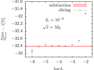
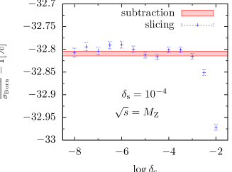
Figure 9: Slicing cut dependence of $\sigma_{\mathrm{had}}\left(M_{\mathrm{Z}}\right)$. For comparison also the results of the subtraction method are shown.

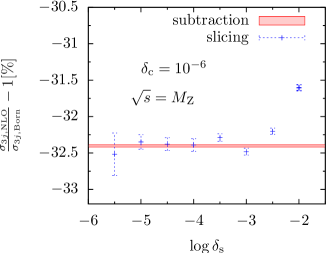
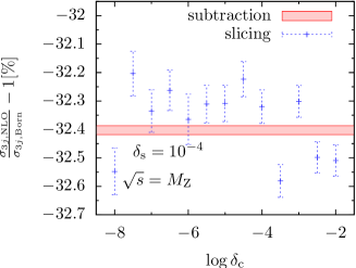
Figure 10: Dependence of the three-jet rate on the slicing parameters at $\sqrt{s}=M_{\mathrm{Z}}$ for $y_{\mathrm{cut}}=0.0006$. For comparison also the results of the subtraction method are shown.

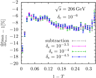
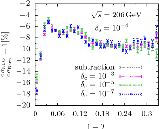
Figure 11: Dependence of the differential thrust distribution on the slicing parameters at $\sqrt{s}=206\,\mathrm{GeV}$. For comparison also the results of the subtraction method are shown.

We find that within integration errors the slicing results become independent of the cut-offs for $\delta_{s}\lesssim 10^{-3}$ and $\delta_{c}\lesssim 10^{-4}$ and fully agree with the results obtained using the subtraction method. For the sake of clarity, we show only curves for values of the slicing parameters that lie on the plateau in Fig. 11. For values of the slicing parameters outside the plateau, the behaviour follows the same pattern as in Figs. 9 and 10.

It turns out that the subtraction method is more efficient in terms of run-time compared to phase-space slicing. To obtain results of comparable statistical quality, the phase-space slicing method required about one order of magnitude more events than the subtraction method. We therefore used the subtraction method to obtain the results presented in the following sections, both for $\sigma_{\mathrm{had}}$ and jet rates and event-shape distributions.

6 Numerical results

The numerical parton-level event generator described above can be used to compute the ${\cal O}(\alpha)$ electroweak corrections to the total hadronic cross section, to event-shape distributions, and to the three-jet rate.

6.1 Results for the total hadronic cross section

	$\sqrt{s}=M_{\mathrm{Z}}$	$\frac{{\mathrm{d}}\sigma_{i}-{\mathrm{d}}\sigma_{\mathrm{Born}}}{{\mathrm{d}}\sigma_{\mathrm{Born}}}[\%]$	$\sqrt{s}=133\,\mathrm{GeV}$	$\frac{{\mathrm{d}}\sigma_{i}-{\mathrm{d}}\sigma_{\mathrm{Born}}}{{\mathrm{d}}\sigma_{\mathrm{Born}}}[\%]$
$\sigma_{\mathrm{had}}^{\mathrm{Born}}/\,\mathrm{nb}$	$38.2845(15)$		$0.068858(2)$
$\sigma_{\mathrm{had}}^{\mathrm{weak}}/\,\mathrm{nb}$	$37.8541(2)$	$~{}{-1.1}$	$0.068348(2)$	$-0.7$
$\sigma_{\mathrm{had}}^{\mathrm{NLO}}/\,\mathrm{nb}$	$25.729(3)$	$-32.8$	$0.06269(2)$	$-9.0$
$\sigma_{\mathrm{had}}^{\mathrm{NLO+h.o.LL}}/\,\mathrm{nb}$	$27.341(3)$	$-28.6$	$0.06208(2)$	$-9.8$

	$\sqrt{s}=172\,\mathrm{GeV}$	$\frac{{\mathrm{d}}\sigma_{i}-{\mathrm{d}}\sigma_{\mathrm{Born}}}{{\mathrm{d}}\sigma_{\mathrm{Born}}}[\%]$	$\sqrt{s}=206\,\mathrm{GeV}$	$\frac{{\mathrm{d}}\sigma_{i}-{\mathrm{d}}\sigma_{\mathrm{Born}}}{{\mathrm{d}}\sigma_{\mathrm{Born}}}[\%]$
$\sigma_{\mathrm{had}}^{\mathrm{Born}}/\,\mathrm{nb}$	$0.0276993(8)$		$0.0170486(5)$
$\sigma_{\mathrm{had}}^{\mathrm{weak}}/\,\mathrm{nb}$	$0.0276780(8)$	$~{}{-0.1}$	$0.0170626(5)$	$~{}0.1$
$\sigma_{\mathrm{had}}^{\mathrm{NLO}}/\,\mathrm{nb}$	$0.024770(7)$	$-10.6$	$0.015197(4)$	$-10.9$
$\sigma_{\mathrm{had}}^{\mathrm{NLO+h.o.LL}}/\,\mathrm{nb}$	$0.024633(7)$	$-11.1$	$0.015127(4)$	$-11.3$

	$\sqrt{s}=500\,\mathrm{GeV}$	$\frac{{\mathrm{d}}\sigma_{i}-{\mathrm{d}}\sigma_{\mathrm{Born}}}{{\mathrm{d}}\sigma_{\mathrm{Born}}}[\%]$	$\sqrt{s}=1000\,\mathrm{GeV}$	$\frac{{\mathrm{d}}\sigma_{i}-{\mathrm{d}}\sigma_{\mathrm{Born}}}{{\mathrm{d}}\sigma_{\mathrm{Born}}}[\%]$
$\sigma_{\mathrm{had}}^{\mathrm{Born}}/\,\mathrm{nb}$	$0.00241881(7)$		$0.00059139(2)$
$\sigma_{\mathrm{had}}^{\mathrm{weak}}/\,\mathrm{nb}$	$0.00238722(7)$	$~{}{-1.3}$	$0.00056838(2)$	$~{}{-3.9}$
$\sigma_{\mathrm{had}}^{\mathrm{NLO}}/\,\mathrm{nb}$	$0.0020665(7)$	$-14.6$	$0.0004856(2)$	$-17.9$
$\sigma_{\mathrm{had}}^{\mathrm{NLO+h.o.LL}}/\,\mathrm{nb}$	$0.0020585(7)$	$-14.9$	$0.0004836(2)$	$-18.2$

Table 1: Total hadronic cross section $\sigma_{\mathrm{had}}\left(\sqrt{s}\right)$ for LEP1 and LEP2 energies, and for $\sqrt{s}=500\,\mathrm{GeV}$ and $\sqrt{s}=1\,\mathrm{TeV}$.

The total hadronic cross section as a function of the CM energy and the corresponding NLO electroweak corrections have been shown in Ref. [24]. Here we list some numbers that have been used to extract $\delta_{\sigma,1}$ and $\delta_{\sigma,\geq 2,\mathrm{LL}}$, as defined in (2.17) and (2.21), which enter the calculation of normalised event-shape distributions and jet rates. We use the event selection as described in Section 5.1 with the cut parameters given in (5.11). In the following, ‘weak’ refers to the electroweak NLO corrections without purely photonic corrections.

Table 1 shows the Born contribution to $\sigma_{\mathrm{had}}$ in the first row, the weak $\mathcal{O}(\alpha)$ contribution in the second row, the full $\mathcal{O}(\alpha)$ contribution in the third row, and the full $\mathcal{O}(\alpha)+$ h.o. LL contribution in the fourth row for LEP1 and LEP2 energies, as well as for $\sqrt{s}=500\,\mathrm{GeV}$ and $\sqrt{s}=1000\,\mathrm{GeV}$. We show the absolute results in nanobarn in the second and fourth columns and the relative corrections in per cent in the third and fifths columns. The numbers in parentheses give the uncertainties from Monte Carlo integration in the last digits of the predictions. For most energies, the electroweak corrections are sizable and negative, ranging between $-30\%$ at the $\mathrm{Z}$ peak and about $-9\%$ at energies above. The numerically largest contribution is always due to ISR. Above $120\,\mathrm{GeV}$ the magnitude of the corrections is increased due to LL resummation of ISR, whereas it is decreased in the resonance region. The virtual one-loop weak corrections (from fermionic and massive bosonic loops) are moderate of a few per cent and always negative for $M_{\mathrm{Z}}<\sqrt{s}<1\,\mathrm{TeV}$.

6.2 Results for the event-shape distributions and jet rates

In the following we present the results of our calculation for the three-jet rate as well as for event-shape distributions as described in Section 2. We show our findings for $\sqrt{s}=M_{\mathrm{Z}}$ as used at LEP1 and the selected LEP2 energies $172\,\mathrm{GeV}$ and $206\,\mathrm{GeV}$. To stress the relevance of our work for future linear colliders, we also show results for $\sqrt{s}=500\,\mathrm{GeV}$.

The precise size and shape of the corrections depend on the observable $y$ in question. However, they share the common feature that $q\bar{q}\gamma$ final states contribute only in the two-jet region, typically for small values of $y$.

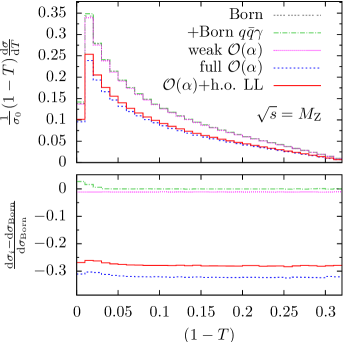
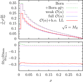
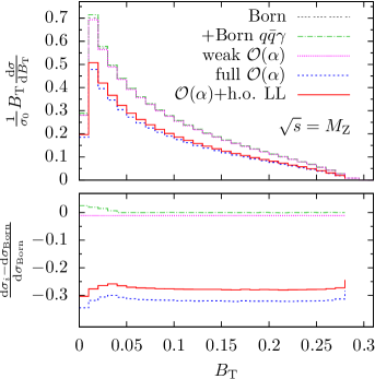
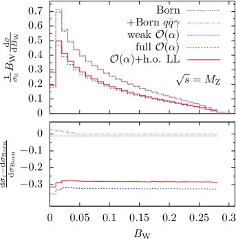
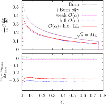
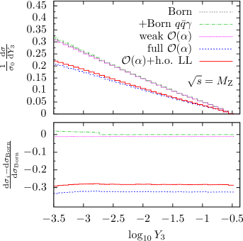
Figure 12: The event-shape distributions normalised to $\sigma_{0}$ at $\sqrt{s}=M_{\mathrm{Z}}$.

In a first step, we show our results for the distributions normalised to $\sigma_{0}$ for $\sqrt{s}=M_{\mathrm{Z}}$ in Fig. 12. The Born contribution is given by the $A$ term of (2.18), while the full ${\cal O}(\alpha)$ corrections contain the tree-level $q\bar{q}\gamma$ contribution $\delta_{\gamma}$ and the NLO electroweak contribution $\delta_{A}$ of (2.18). The $T$, $\rho$, $B_{\mathrm{T}}$, $B_{\mathrm{W}}$, and $C$ distributions are weighted by the respective variable $y$, evaluated at each bin centre. The relative corrections in the lower boxes are obtained by dividing the respective contributions to the corrections by the Born distribution given by the $A$ term. We observe large negative corrections due to ISR, and moderate weak corrections in all distributions. The corrections are mainly constant for large $y$ (note that we plot $1-T$ instead of $T$), where the isolated-photon veto rejects all contributions from $q\bar{q}\gamma$ final states. Near the two-jet limit, the contribution from $q\bar{q}\gamma$ final states dominates the relative corrections. Moreover, it turns out that the electromagnetic corrections depend non-trivially on the event-selection cuts (see Section 6.3 for a more detailed discussion). We observe a significant decrease from the second bin to the first bin in all distributions, caused by the lower cut-off that we impose individually for all distributions. Since the cut-off acts both in the Born and the NLO contribution, we find a meaningful result for the relative corrections in the first bin. In the $Y_{3}$ distribution we clearly see the onset of the $q\bar{q}\gamma$ final states for $Y_{3}=0.002$. Since we always cluster photons with $y<y_{\mathrm{cut}}=0.002$ in the event selection (see Section 5.1), the contribution from $q\bar{q}\gamma$ final states is removed if $Y_{3}>0.002$ and only plays a role for $Y_{3}<0.002$.

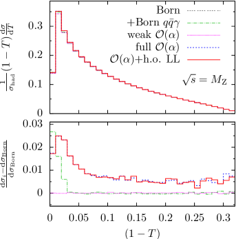
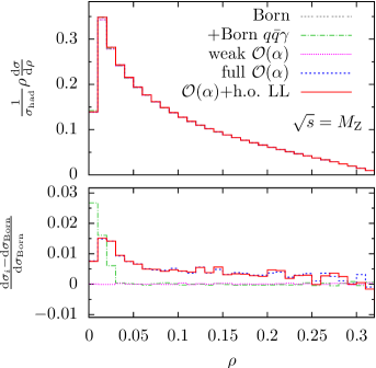
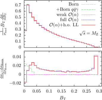
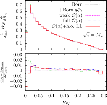
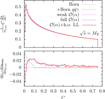
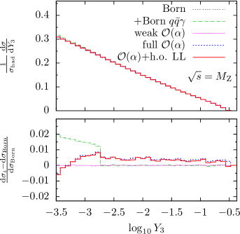
Figure 13: The event-shape distributions normalised to $\sigma_{\mathrm{had}}$ at $\sqrt{s}=M_{\mathrm{Z}}$.

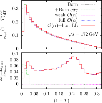
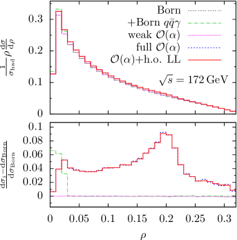
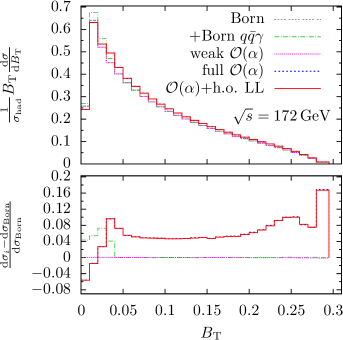
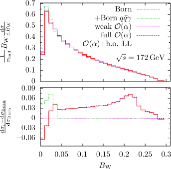
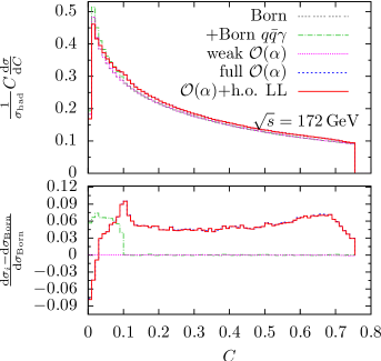
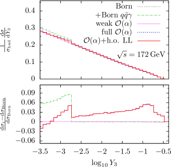
Figure 14: The event-shape distributions normalised to $\sigma_{\mathrm{had}}$ at $\sqrt{s}=172\,\mathrm{GeV}$.

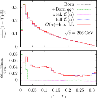
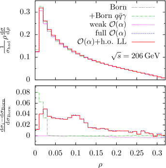
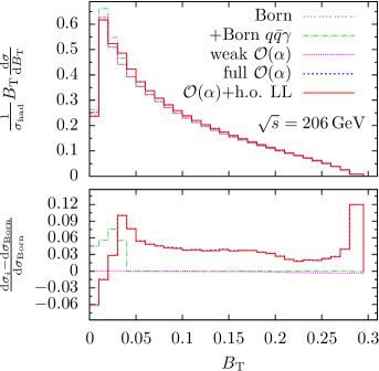
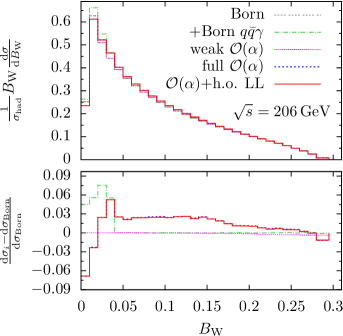
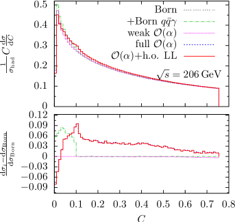
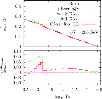
Figure 15: The event-shape distributions normalised to $\sigma_{\mathrm{had}}$ at $\sqrt{s}=206\,\mathrm{GeV}$.

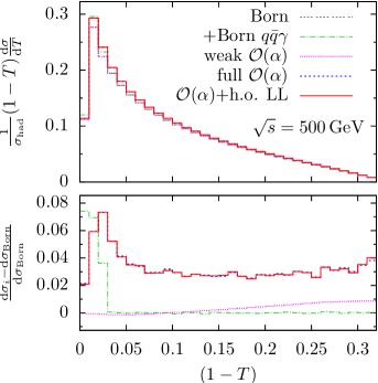
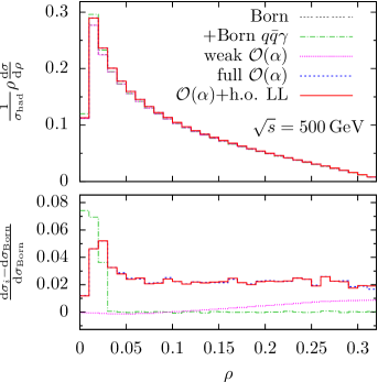
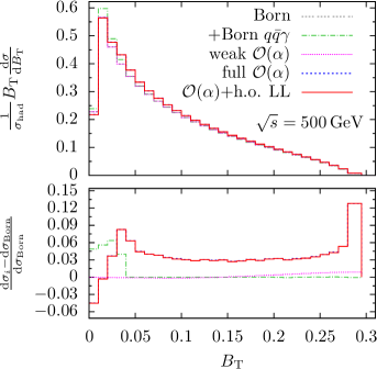
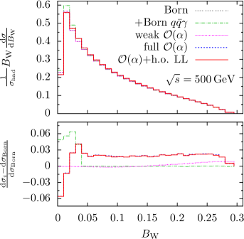
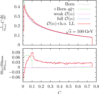
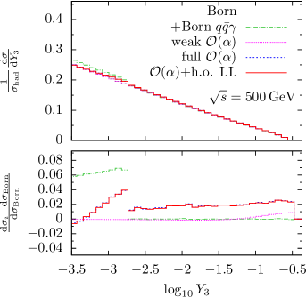
Figure 16: The event-shape distributions normalised to $\sigma_{\mathrm{had}}$ at $\sqrt{s}=500\,\mathrm{GeV}$.

In expanding the corrections according to (2.19), and retaining only terms up to LO in $\alpha_{\mathrm{s}}$, we obtain the genuine electroweak corrections to normalised event-shape distributions, which we display at $\sqrt{s}=M_{\mathrm{Z}}$ in Fig. 13. The Born contribution is given by the $A$ term of (2.19), while the ${\cal O}(\alpha)$ corrections are now given by $\delta_{\mathrm{EW}}$ of (2.20). It can be seen very clearly that the large ISR corrections cancel between the event-shape distributions and the hadronic cross section when expanding the normalised distributions properly, resulting in electroweak corrections of a few per cent. Moreover, effects from ISR resummation are largely reduced as well, and the difference between $\mathcal{O}{\left(\alpha\right)}$ and $\mathcal{O}{\left(\alpha\right)}+{}$ h.o. LL is very small. The purely weak corrections are below the per-mille level.

For the thrust distribution, the full $\mathcal{O}{\left(\alpha\right)}$ corrections are almost constant around $0.5\%$ for $(1-T)>0.05$. The coefficient $\delta_{\gamma}$ starts to emerge for $(1-T)=0.04$ and contributes up to $2.6\%$. The full $\mathcal{O}(\alpha)$ corrections peak for $(1-T)=0.02$ at $2.5\%$ and amount to $1.8\%$ for $(1-T)=0.01$ in the first bin. The full $\mathcal{O}(\alpha)$ corrections are flat and around $0.5\%$ for $\rho>0.05$, $B_{\mathrm{W}}>0.05$, $C>0.1$, and $Y_{3}>0.002$. For the $B_{\mathrm{T}}$ distribution they are around $1\%$ and almost flat for $B_{\mathrm{T}}>0.05$. The full $\mathcal{O}{\left(\alpha\right)}$ corrections reach a maximum between 1% and 3% typically for small values of the event-shape variables and drop towards the first bin down to between $1.8\%$ and $-4.1\%$. Only for $B_{\mathrm{T}}$ we find also a maximum (of $4\%$) in the last bin. The LO $q\bar{q}\gamma$ channel contributes only for small $y$ and can amount up to 4%.

In Fig. 14 we show our results for $\sqrt{s}=172\,\mathrm{GeV}$. The behaviour is similar as for $\sqrt{s}=M_{\mathrm{Z}}$, but in the middle of the distributions a peaking structure emerges. It is located at $1-T,\rho,B_{\mathrm{W}}\approx 0.2$, $B_{\mathrm{T}}\approx 0.25$, $C\approx 0.65$, and $Y_{3}\approx 0.1$. We investigate this behaviour in detail in the next section. In all event-shape distributions the LO $q\bar{q}\gamma$ contribution ranges between $3\%$ and $8\%$. Outside the two-jet region and apart from the domain of the peaking structure, the full $\mathcal{O}{\left(\alpha\right)}$ corrections are flat and of the order of $5\%$. They peak near the onset of the $q\bar{q}\gamma$ final states between $4\%$ and $10\%$, and drop in the first bin down to between $1.5\%$ and $-10\%$.

Results for $\sqrt{s}=206\,\mathrm{GeV}$, are displayed in Fig. 15. In all event-shape distributions the LO $q\bar{q}\gamma$ contribution ranges between $4\%$ and $9\%$. Outside the two-jet region and outside the domain where the peaking structure is located, the full $\mathcal{O}{\left(\alpha\right)}$ corrections are flat between $0.1\%$ and $2\%$, they peak near the onset of the $q\bar{q}\gamma$ final states between $5\%$ and $9\%$, and drop in the first bin down to between $2\%$ and $-8\%$. The peaking structure is now situated at smaller values of $y$, it is less pronounced and, especially for $B_{\mathrm{W}}$, $B_{\mathrm{T}}$, $C$, and $Y_{3}$, it extends over a larger range of $y$. Additionally, for large values of $y$, the weak contribution slightly increases.

Finally, in Fig. 16 we show our results for $\sqrt{s}=500\,\mathrm{GeV}$. In the event-shape distributions the LO $q\bar{q}\gamma$ contribution ranges between $2\%$ and $8\%$. Outside the two-jet region, the full $\mathcal{O}{\left(\alpha\right)}$ corrections are flat between $2\%$ and $3\%$, they peak near the onset of the $q\bar{q}\gamma$ final states between $2\%$ and $9\%$, and drop in the first bin down to between $2\%$ and $-6\%$. The weak corrections here contribute up to $+1\%$ in all observables for large values of $y$. The peaking structure as observed for $\sqrt{s}=172\,\mathrm{GeV}$ and $\sqrt{s}=206\,\mathrm{GeV}$ has completely disappeared.

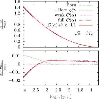
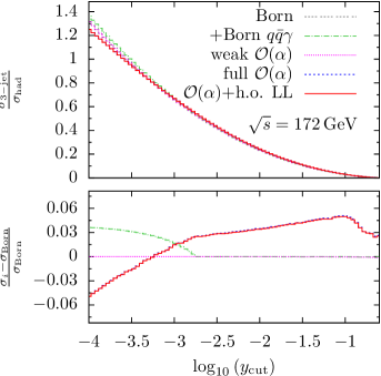
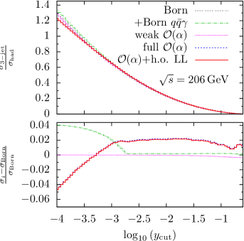
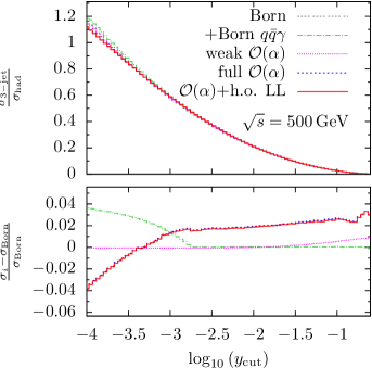
Figure 17: The three-jet rate normalised to $\sigma_{\mathrm{had}}$ at different CM energies.

Figure 17 displays the corrections to the three-jet rate at various CM energies. As above, the corrections are appropriately normalised to $\sigma_{\mathrm{had}}$. At $\sqrt{s}=M_{\mathrm{Z}}$, the full $\mathcal{O}{\left(\alpha\right)}$ corrections to the three-jet rate are about $0.5\%$ for $y_{\mathrm{cut}}\gtrsim 0.002$. Because we use $y_{\mathrm{cut}}=0.002$ in the event selection, $q\bar{q}\gamma$ final states contribute only if $y_{\mathrm{cut}}\lesssim 0.002$. The LO $q\bar{q}\gamma$ contribution amounts to $1\%$. For $y_{\mathrm{cut}}<0.002$, the full $\mathcal{O}{\left(\alpha\right)}$ corrections become negative, reaching $-1.5\%$ in the first bin. For $y_{\mathrm{cut}}\lesssim 0.0005$ the three-jet rate becomes larger than $\sigma_{\mathrm{had}}$. This behaviour indicates the breakdown of the perturbative expansion in $\alpha_{\mathrm{s}}$ due to large logarithmic corrections proportional to $\log(y_{\mathrm{cut}})$ at all orders. Inclusion of higher-order QCD corrections, which are large and negative [17, 18] in this region, yields a ratio of $\sigma_{\mbox{\scriptsize 3-jet}}$ to $\sigma_{\mathrm{had}}$ less than unity for an extended range of $\log(y_{\mathrm{cut}})$. At the higher CM energies, the corrections to the three-jet rate are larger than at $\sqrt{s}=M_{\mathrm{Z}}$. For $y_{\mathrm{cut}}\gtrsim 0.002$, they are almost constant and amount to about 4% at $172\,\mathrm{GeV}$, and about 2% at $206\,\mathrm{GeV}$ and $500\,\mathrm{GeV}$. In the region $y_{\mathrm{cut}}<0.002$, we find a negative contribution of up to $-5\%$ for very small values of $y_{\mathrm{cut}}$.

6.3 Impact of the event-selection cuts on the event-shape distributions

In the above results, we could clearly observe that the electroweak corrections to event-shape distributions are not flat, but display peak structures. These structures are most pronounced at $\sqrt{s}=172\,\mathrm{GeV}$. They are discussed here for thrust as an example. In Fig. 14, we see that the relative corrections show a peaking structure for $1-T\approx 0.2$. To understand the origin of these structures, we extensively studied how variations of the event-selection cuts, especially the hard-photon cut, influence the event-shape distributions.

We employ three different cuts in our calculation which depend on four parameters:

• A cut on the production angle $\theta_{i}$ of all particles, such that only particles $i$ with $\cos\theta_{i}>\cos\theta_{\mathrm{cut}}$ are used in the reconstruction of the event-shape variables. By default, we use the value $\cos\theta_{\mathrm{cut}}=0.965$.

• A cut on the visible energy squared $s^{\prime}$ of the final state, such that only events with $s^{\prime}>s_{\mathrm{cut}}$ are accepted. By default, we use the value $s_{\mathrm{cut}}=0.81s$.

• The maximum photon energy in a jet $z$, for which we require $z<z_{\mathrm{cut}}$, where the particles are clustered according to the Durham jet algorithm with parameter $y_{\mathrm{cut}}$. By default, we use the values $z_{\mathrm{cut}}=0.9$ and $y_{\mathrm{cut}}=0.002$.

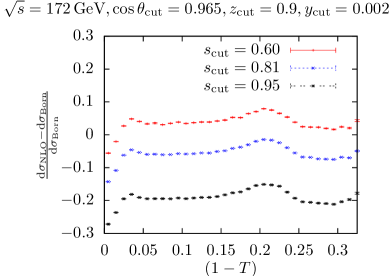
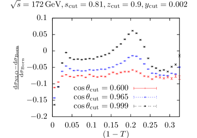
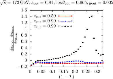
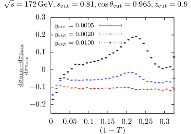
Figure 18: Dependence of the thrust distribution on different values of the phase-space cuts at $\sqrt{s}=172\,\mathrm{GeV}$.

In Fig. 18 we show the full $\mathcal{O}{\left(\alpha\right)}$ corrections to the thrust distribution normalised to the Born contribution for $\sqrt{s}=172\,\mathrm{GeV}$, where the peak structures are most striking. We plot the results for three different values of a single cut parameter while we set the other three cut parameters to their default value. Going from left to right and top to bottom, we vary $s_{\mathrm{cut}}$, $\cos\theta_{\mathrm{cut}}$, $z_{\mathrm{cut}}$, and $y_{\mathrm{cut}}$. By changing $s_{\mathrm{cut}}$ we observe a change in normalisation of about $25\%$, while the shape of the distribution stays the same. Varying $\cos\theta_{\mathrm{cut}}$ from larger to smaller values leads to a more and more pronounced peak at $(1-T)\simeq 0.2$. The corrections grow below the peak but are only slightly changed above. The different slopes for $1-T<0.03$ result from the changing acceptance of ISR photons. Modifying $z_{\mathrm{cut}}$ has a dramatic effect on the peak. For $z_{\mathrm{cut}}=0.99$ we find a very pronounced resonance for $(1-T)\simeq 0.28$. By reducing the cut, the resonance gets strongly suppressed and moves to smaller values of $(1-T)$. By increasing $y_{\mathrm{cut}}$, we observe an enhancement of the peak, as well as a slight shift towards larger values of $1-T$.

In Fig. 19 we study the change of the $\mathcal{O}{\left(\alpha\right)}$ corrections to the thrust distribution normalised to the Born contribution with $z_{\mathrm{cut}}$ for $\sqrt{s}=M_{\mathrm{Z}}$, $133\,\mathrm{GeV}$, $206\,\mathrm{GeV}$, and $500\,\mathrm{GeV}$.

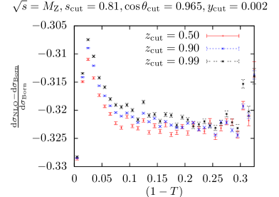
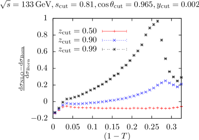
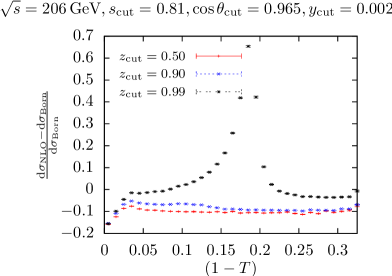
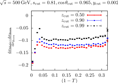
Figure 19: Dependence of the thrust distribution on different values of the cut $z_{\mathrm{cut}}$ at $\sqrt{s}=M_{\mathrm{Z}}$, $133\,\mathrm{GeV}$, $206\,\mathrm{GeV}$, and $500\,\mathrm{GeV}$.

Varying $z_{\mathrm{cut}}$ for $\sqrt{s}=M_{\mathrm{Z}}$ leaves the distribution basically unchanged. By increasing $z_{\mathrm{cut}}$ from 0.5 to 0.99 for $\sqrt{s}=133\,\mathrm{GeV}$ we find a growth of the peak to almost $100\%$. We also observe that the peak moves from $1-T\approx 0.28$ for $z_{\mathrm{cut}}=0.9$ to $1-T\approx 0.25$ for $z_{\mathrm{cut}}=0.99$. For $\sqrt{s}=206\,\mathrm{GeV}$ we see the same features as for $\sqrt{s}=172\,\mathrm{GeV}$, but now with the peak at $(1-T)\simeq 0.19$ for large $z_{\mathrm{cut}}$. Finally, for $\sqrt{s}=500\,\mathrm{GeV}$ a peaking structure seems to appear at $(1-T)\simeq 0.03$, while varying $z_{\mathrm{cut}}$ basically changes only the normalisation.

Through analysing events at the level of the Monte Carlo generator, we find that the enhancement in the region of the peaking structure always stems from $q\bar{q}\mathrm{g}\gamma$ final states, where a soft gluon is clustered with a hard photon. Increasing $\cos\theta_{\mathrm{cut}}$ leads to a logarithmic enhancement of collinear ISR photons, increasing $z_{\mathrm{cut}}$ generally results in a larger acceptance of photons inside jets, and increasing $y_{\mathrm{cut}}$ causes more photons to be clustered together with other partons, resulting in less events with isolated photons being removed. We can therefore conclude that the peaking structure results from the ISR photon contribution, where a soft gluon is clustered together with the photon.

More precisely, the peaking structure can be explained by the radiative-return phenomenon. Since we do not remove all energetic photons, it is possible that a hard photon and a soft gluon are clustered together, such that the energy fraction of the photon in the jet does not exceed $z_{\mathrm{cut}}$ and the invariant mass of the quark–antiquark–gluon system $s_{q{\bar{q}}g}$ is equal to the mass of the $\mathrm{Z}$ boson. Such a configuration leads on the one hand to an enhancement due to radiative return but also to a logarithmic enhancement due to the soft gluon.

In order to analyse this effect further, we consider events where the photon and the soft gluon are clustered together, such that we have a three-particle final state that consists of a quark, an antiquark, and a photonic jet. Assume that the quark, antiquark, and the photonic jet have the three-momenta $\vec{p}_{q},\vec{p}_{\bar{q}},\vec{p}_{\gamma}$ and the energies $E_{q},E_{\bar{q}},E_{\gamma}$, respectively. We use energy-momentum conservation

$$\vec{p}_{q}+\vec{p}_{\bar{q}}+\vec{p}_{\gamma} = 0,$$

$$E_{q}+E_{{\bar{q}}}+E_{\gamma} = \sqrt{s}.$$ (6.1)

and demand that the invariant mass of the quark–antiquark pair is equal to $M_{\mathrm{Z}}$, such that

$$s_{q{\bar{q}}}=\left(E_{q}+E_{\bar{q}}\right)^{2}-\left(\vec{p}_{q}+\vec{p}_{\bar{q}}\right)^{2}=\left(E_{q}+E_{\bar{q}}\right)^{2}-\left(\vec{p}_{\gamma}\right)^{2}=\left(E_{q}+E_{\bar{q}}\right)^{2}-E_{\gamma}^{2}=M_{\mathrm{Z}}^{2}.$$ (6.2)

Energy conservation (6.1) and the mass-shell condition (6.2) imply

$$E_{q}+E_{\bar{q}}=\frac{s+M_{\mathrm{Z}}^{2}}{2\sqrt{s}},\qquad E_{\gamma}=\frac{s-M_{\mathrm{Z}}^{2}}{2\sqrt{s}}.$$ (6.3)

It can be shown that in a three-jet configuration with massless partons, thrust is always determined by the energy of the most energetic particle $E_{\mathrm{max}}$ [27], i.e.

$$T=\frac{2E_{\mathrm{max}}}{\sqrt{s}}.$$ (6.4)

If we now assume that the quark and the antiquark carry the same energy, we can calculate the energies of all three jets in the final state at different energies:

$$E_{q}\left(133\,\mathrm{GeV}\right)=E_{\bar{q}}\left(133\,\mathrm{GeV}\right)\approx~{}49\,\mathrm{GeV},\quad E_{\gamma}\left(133\,\mathrm{GeV}\right) \!\approx\! ~{}35\,\mathrm{GeV},$$

$$E_{q}\left(172\,\mathrm{GeV}\right)=E_{\bar{q}}\left(172\,\mathrm{GeV}\right)\approx~{}55\,\mathrm{GeV},\quad E_{\gamma}\left(172\,\mathrm{GeV}\right) \!\approx\! ~{}62\,\mathrm{GeV},$$

$$E_{q}\left(206\,\mathrm{GeV}\right)=E_{\bar{q}}\left(206\,\mathrm{GeV}\right)\approx~{}61\,\mathrm{GeV},\quad E_{\gamma}\left(206\,\mathrm{GeV}\right) \!\approx\! ~{}84\,\mathrm{GeV},$$

$$E_{q}\left(500\,\mathrm{GeV}\right)=E_{\bar{q}}\left(500\,\mathrm{GeV}\right)\approx 129\,\mathrm{GeV},\quad E_{\gamma}\left(500\,\mathrm{GeV}\right) \!\approx\! 242\,\mathrm{GeV}.$$ (6.5)

This leads to the following thrust values where the radiative-return phenomena should appear:

$$(1-T_{\mathrm{RR}})(\sqrt{s}=133\,\mathrm{GeV})\approx 0.27,$$

$$(1-T_{\mathrm{RR}})(\sqrt{s}=172\,\mathrm{GeV})\approx 0.28,$$

$$(1-T_{\mathrm{RR}})(\sqrt{s}=206\,\mathrm{GeV})\approx 0.19,$$

$$(1-T_{\mathrm{RR}})(\sqrt{s}=500\,\mathrm{GeV})\approx 0.03.$$ (6.6)

These values coincide perfectly with the peaks in Figs. 18 and 19. Relaxing the assumption that the quark and the antiquark carry the same energy only results in a broadening of the peaking structure. Varying the value of $z_{\mathrm{cut}}$ leads to different energies of the photonic jet and therefore changes the allowed energies in the above analysis. For decreasing values of $z_{\mathrm{cut}}$, we therefore either only observe the tail of the peak or cut it away completely which effectively looks like a shift of the position or the disappearance of the peak. For $\sqrt{s}=133\,\mathrm{GeV}$ we observe the tail of the peak for $E_{q}<E_{q,\mathrm{peak}}$ such that for decreasing $z_{\mathrm{cut}}$ the peak seems to move to larger values of $(1-T)$. For $\sqrt{s}=172\,\mathrm{GeV}$ and $\sqrt{s}=206\,\mathrm{GeV}$ we observe the tail of the peak for $E_{\gamma}>E_{\gamma,\mathrm{peak}}$ such that for decreasing $z_{\mathrm{cut}}$ the peak seems to move to smaller values of $(1-T)$.

The study in this section clearly illustrates the non-trivial effect of realistic photon isolation criteria to the electroweak corrections to jet observables. The accidental clustering of a soft gluon with a hard photon results in a photon jet with a photon energy fraction below the rejection cut. In these events, the distribution of the final-state jets, and their reconstructed pair invariant masses do no longer reflect the underlying parton dynamics. A similar misreconstruction could also happen for electroweak corrections to final states involving jets at hadron colliders, and clearly deserves further study.

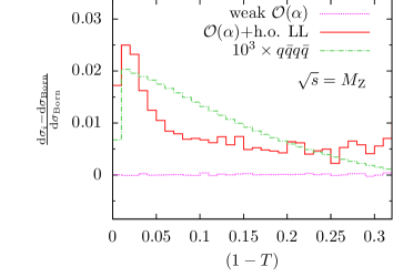
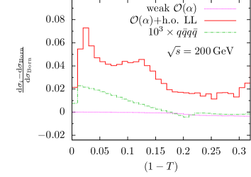
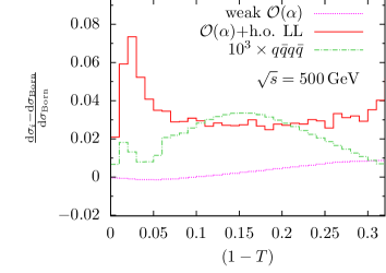
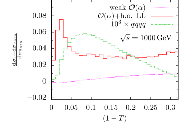
Figure 20: Electroweak corrections to the thrust distribution at different CM energies. The interference contribution between electroweak and QCD diagrams for the four-quark final state is scaled by a factor 1000.

6.4 Contribution from four-quark final states

At ${\cal O}(\alpha^{3}\alpha_{\mathrm{s}})$, event-shape distributions and jet cross sections receive a contribution from the process $\mathrm{e}^{+}\mathrm{e}^{-}\to q\bar{q}q\bar{q}$ through the interference of QCD and electroweak amplitudes [see (3.23)]. Compared to other contributions at this order, this four-quark interference contribution is very small. Its typical magnitude amounts to about one per mille of the electroweak correction, and is thus within the integration error of the four-particle contribution. To illustrate the smallness of this contribution, Fig. 20 compares the four-quark contribution (scaled by a factor 1000) to the total electroweak correction to the normalised thrust distribution at different CM energies. The relative magnitude of the four-quark contribution is always at the per-mille level.

7 Conclusions and outlook

In this paper, we have derived the NLO electroweak corrections to three-jet production and event-shape distributions in $\mathrm{e}^{+}\mathrm{e}^{-}$ annihilation. At this order, contributions arise from virtual corrections from weak gauge bosons (which were evaluated in the complex-mass scheme to take proper account of the gauge-boson widths), from fermionic loops, from real and virtual photonic corrections and from interferences between electroweak and QCD diagrams for four-quark final states.

Our calculation is one of the first to address electroweak corrections to jet production observables. For this type of observables, one has to take proper account of the experimental event-selection cuts, which are aiming to reject events containing isolated photons. An infrared-safe definition of isolated photons must permit some amount of hadronic energy around the photon; for jet observables, this can be realized by a democratic clustering procedure, used by the LEP experiments. In this approach, the photon is clustered like any other hadron by the jet algorithm, resulting in a photon jet. If the photon carries more than a predefined large fraction of the jet energy, it is called isolated and the event is discarded. In our calculation, we have implemented this isolated-photon-veto procedure. Since it involves cuts on a specific, identified particle in the final state, the resulting observable is no longer collinear-safe, and the left-over collinear singularity is compensated by a further contribution from the quark-to-photon fragmentation function. We have documented this part of the calculation in detail in different schemes.

The NLO electroweak corrections to absolute cross sections and event-shape distributions turn out to be numerically substantial: for example for thrust at $\sqrt{s}=M_{\mathrm{Z}}$, they amount to a correction of $-32\%$, which is largely dominated by initial-state radiation. Beyond the NLO electroweak corrections, we also included higher-order leading logarithmic corrections, which are sizable. Their inclusion at $\sqrt{s}=M_{\mathrm{Z}}$ results in a total correction of $-28\%.$ Normalizing these results to the total hadronic cross section (as is done in the experimental measurement), corrected to the same order, only very moderate corrections remain in the normalized jet cross sections and event distributions, and practically no difference is observed between the fixed-order NLO electroweak results and the results including higher-order logarithmic corrections.

At LEP1, we find that NLO electroweak effects to event-shape distributions amount to a correction of about one to two per cent. The corrections are not uniform over the kinematical range, but tend to increase towards the two-jet region, where the isolated-photon veto becomes less efficient. The corrections to the three-jet rate are below one per cent. Purely weak contributions form a gauge-invariant subset of the electroweak corrections. At LEP1, these corrections are below the per-mille level.

At LEP2 energies, the NLO electroweak corrections to event-shape distributions and to the three-jet rate are typically at the level of two to eight per cent. The largest contribution comes again from the photonic corrections. These are very sensitive to the precise photon isolation cuts applied to select the events, and are not uniform over the range of event-shape variables. The NLO electroweak event-shape distributions display peaks at LEP2 energies. These peaks are due to a remant of the radiative-return phenomenon, which is not fully suppressed by the photon isolation cuts. The position and energy dependence of these peaks can be explained quantitatively.

Event-shape and jet cross section data from LEP1 and LEP2 have been corrected for photonic radiation effects using multi-purpose leading-logarithmic event generator programs. To compare our results with the experimental data would first require to undo these corrections. A further complication in the comparison with data arises from the fact that event-shape distributions at LEP2 were determined in the $\mathrm{e}^{+}\mathrm{e}^{-}$ centre-of-mass frame for all events, including initial-state-radiation events. Most of the event-shape variables are not boost invariant, and should thus be reconstructed in the centre-of-mass frame of the observed hadrons. If reconstructed in the $\mathrm{e}^{+}\mathrm{e}^{-}$ centre-of-mass frame, ideal two-jet events with initial-state radiation will not be placed at the kinematical edge of the distribution, thus violating infrared-safety criteria. Within a perturbative calculation, it is not possible to apply the event reconstruction in the $\mathrm{e}^{+}\mathrm{e}^{-}$ centre-of-mass frame. The purely weak corrections at LEP1 and LEP2 were previously not accounted for in the interpretation of event-shape and jet cross section data. Our study shows that they are at the level of one per mille or below for appropriately normalized distributions. At the current level of experimental and theoretical precision, they are thus not yet relevant to precision QCD studies of LEP data.

While the magnitude of electroweak corrections decreases towards higher LEP2 energies, we observe them to increase again when going to even higher energies, corresponding to a future linear collider. In part, this increase comes from the fact that purely weak corrections (which were negligible throughout the LEP2 energy range) become sizable at high energies. At $\sqrt{s}=500$ GeV, NLO electroweak corrections to event-shape distributions and jet cross sections amount to two to four per cent, and have thus a potentially sizable impact on precision QCD studies at a future linear collider. The purely weak corrections reach up to one per cent at this energy. Most importantly, our findings on the interplay of photon isolation and event-selection cuts, and on the appropriate frame for the reconstruction of initial-state radiation events will help to optimize precision QCD studies at future high-energy $\mathrm{e}^{+}\mathrm{e}^{-}$ colliders from event shapes and jet cross sections.

References

-
[1]
D.J. Gross and F. Wilczek, Phys. Rev. D 8 (1973) 3633;
H.D. Politzer, Phys. Rept. 14 (1974) 129;
H. Fritzsch, M. Gell-Mann and H. Leutwyler, Phys. Lett. B 47 (1973) 365. -
[2]
R. Brandelik et al. [TASSO Collaboration],
Phys. Lett. B 86 (1979) 243;
P. Söding, B. Wiik, G. Wolf and S.L. Wu, Talks given at Award Ceremony of the 1995 EPS High Energy and Particle Physics Prize, Proceedings of the EPS High Energy Physics Conference, Brussels, 1995, (World Scientific), p. 3. - [3] J. Ellis, M.K. Gaillard and G.G. Ross, Nucl. Phys. B111 (1976) 253; B130 (1977) 516(E).
-
[4]
O. Biebel,
Phys. Rept. 340 (2001) 165;
S. Kluth, Rept. Prog. Phys. 69 (2006) 1771;
S. Bethke, Prog. Part. Nucl. Phys. 58 (2007) 351. -
[5]
D. Buskulic et al. [ALEPH Collaboration],
Z. Phys. C 73 (1997) 409;
A. Heister et al. [ALEPH Collaboration], Eur. Phys. J. C 35 (2004) 457. -
[6]
P. D. Acton et al. [OPAL Collaboration],
Z. Phys. C 59 (1993) 1;
G. Alexander et al. [OPAL Collaboration], Z. Phys. C 72 (1996) 191;
K. Ackerstaff et al. [OPAL Collaboration], Z. Phys. C 75 (1997) 193;
G. Abbiendi et al. [OPAL Collaboration], Eur. Phys. J. C 16 (2000) 185 [hep-ex/0002012];
G. Abbiendi et al. [OPAL Collaboration], Eur. Phys. J. C 40 (2005) 287 [hep-ex/0503051]. -
[7]
M. Acciarri et al. [L3 Collaboration],
Phys. Lett. B 371 (1996) 137;
M. Acciarri et al. [L3 Collaboration], Phys. Lett. B 404 (1997) 390;
M. Acciarri et al. [L3 Collaboration], Phys. Lett. B 444 (1998) 569;
P. Achard et al. [L3 Collaboration], Phys. Lett. B 536 (2002) 217 [hep-ex/0206052];
P. Achard et al. [L3 Collaboration], Phys. Rept. 399 (2004) 71 [hep-ex/0406049]. -
[8]
P. Abreu et al. [DELPHI Collaboration],
Phys. Lett. B 456 (1999) 322;
J. Abdallah et al. [DELPHI Collaboration], Eur. Phys. J. C 29 (2003) 285 [hep-ex/0307048];
J. Abdallah et al. [DELPHI Collaboration], Eur. Phys. J. C 37 (2004) 1 [hep-ex/0406011]. - [9] K. Abe et al. [SLD Collaboration], Phys. Rev. D 51 (1995) 962 [hep-ex/9501003].
-
[10]
P. A. Movilla Fernandez, O. Biebel, S. Bethke, S. Kluth and P. Pfeifenschneider
[JADE Collaboration],
Eur. Phys. J. C 1 (1998) 461
[hep-ex/9708034];
P. Pfeifenschneider et al. [JADE collaboration and OPAL Collaboration], Eur. Phys. J. C 17 (2000) 19 [hep-ex/0001055]. - [11] R.K. Ellis, D.A. Ross and A.E. Terrano, Nucl. Phys. B 178 (1981) 421.
-
[12]
Z. Kunszt,
Phys. Lett. B 99 (1981) 429;
J.A.M. Vermaseren, K.J.F. Gaemers and S.J. Oldham,
Nucl. Phys. B 187 (1981) 301;
K. Fabricius, I. Schmitt, G. Kramer and G. Schierholz, Z. Phys. C 11 (1981) 315. -
[13]
Z. Kunszt and P. Nason, in Z Physics at LEP 1, CERN Yellow Report
89-08, Vol. 1, p. 373;
W. T. Giele and E.W.N. Glover, Phys. Rev. D 46 (1992) 1980;
S. Catani and M. H. Seymour, Phys. Lett. B 378 (1996) 287. -
[14]
S. Catani, L. Trentadue, G. Turnock and B.R. Webber,
Nucl. Phys. B 407 (1993) 3;
A. Banfi, G.P. Salam and G. Zanderighi, JHEP 0201 (2002) 018 [hep-ph/0112156];
R.W.L. Jones, M. Ford, G.P. Salam, H. Stenzel and D. Wicke, JHEP 0312 (2003) 007 [hep-ph/0312016]. - [15] A. Gehrmann-De Ridder, T. Gehrmann, E.W.N. Glover and G. Heinrich, Phys. Rev. Lett. 99 (2007) 132002 [arXiv:0707.1285 [hep-ph]]; JHEP 0712 (2007) 094 [arXiv:0711.4711 [hep-ph]]; JHEP 0905 (2009) 106 [arXiv:0903.4658 [hep-ph]].
- [16] S. Weinzierl, JHEP 0906 (2009) 041 [arXiv:0904.1077 [hep-ph]]; Phys. Rev. D 80 (2009) 094018 [arXiv:0909.5056 [hep-ph]].
- [17] A. Gehrmann-De Ridder, T. Gehrmann, E.W.N. Glover and G. Heinrich, JHEP 0711 (2007) 058 [arXiv:0710.0346]; Phys. Rev. Lett. 100 (2008) 172001 [arXiv:0802.0813 [hep-ph]].
- [18] S. Weinzierl, Phys. Rev. Lett. 101 (2008) 162001 [arXiv:0807.3241 [hep-ph]]; JHEP 0907 (2009) 009 [arXiv:0904.1145 [hep-ph]].
- [19] T. Gehrmann, G. Luisoni and H. Stenzel, Phys. Lett. B 664 (2008) 265 [arXiv:0803.0695 [hep-ph]].
-
[20]
G. Dissertori, et al.,
JHEP 0802 (2008) 040
[arXiv:0712.0327 [hep-ph]];
JHEP 0908 (2009) 036
[arXiv:0906.3436 [hep-ph]];
R.A. Davison and B.R. Webber, Eur. Phys. J. C 59 (2009) 13 [arXiv:0809.3326 [hep-ph]];
S. Bethke, S. Kluth, C. Pahl and J. Schieck [JADE Collaboration], Eur. Phys. J. C 64 (2009) 351 [arXiv:0810.1389 [hep-ph]];
T. Gehrmann, M. Jaquier and G. Luisoni, arXiv:0911.2422 [hep-ph]. - [21] G. Dissertori, et al., Phys. Rev. Lett. 104 (2010) 072002 [arXiv:0910.4283 [hep-ph]].
- [22] T. Becher and M. D. Schwartz, JHEP 07 (2008) 034 [arXiv:0803.0342 [hep-ph]].
- [23] C. M. Carloni-Calame, S. Moretti, F. Piccinini and D. A. Ross, JHEP 0903 (2009) 047 [arXiv:0804.3771 [hep-ph]]; Eur. Phys. J. C 62 (2009) 355 [Erratum-ibid. C 62 (2009) 453] [arXiv:0811.4758 [hep-ph]]; arXiv:0903.0490 [hep-ph].
- [24] A. Denner, S. Dittmaier, T. Gehrmann and C. Kurz, Phys. Lett. B 679 (2009) 219 [arXiv:0906.0372 [hep-ph]].
- [25] K. Koller, T. F. Walsh, and P. M. Zerwas, Zeit. Phys. C2 (1979) 197.
- [26] JADE, S. Bethke et al., Phys. Lett. B213 (1988) 235.
- [27] G. Dissertori, I. G. Knowles, and M. Schmelling, Oxford, UK: Clarendon (2003) 538 p.
- [28] N. Brown and W. J. Stirling, Phys. Lett. B252 (1990) 657.
- [29] S. Catani, Y. L. Dokshitzer, M. Olsson, G. Turnock, and B. R. Webber, Phys. Lett. B269 (1991) 432.
- [30] S. Brandt, C. Peyrou, R. Sosnowski, and A. Wroblewski, Phys. Lett. 12 (1964) 57 .
- [31] E. Farhi, Phys. Rev. Lett. 39 (1977) 1587.
- [32] L. Clavelli and D. Wyler, Phys. Lett. B103 (1981) 383.
- [33] P. E. L. Rakow and B. R. Webber, Nucl. Phys. B191 (1981) 63.
- [34] S. Catani, G. Turnock, and B. R. Webber, Phys. Lett. B295 (1992) 269.
- [35] G. Parisi, Phys. Lett. B74 (1978) 65.
- [36] J. F. Donoghue, F. E. Low, and S.-Y. Pi, Phys. Rev. D20 (1979) 2759.
- [37] N. Brown and W. J. Stirling, Z. Phys. C53 (1992) 629.
- [38] S. Bethke, Z. Kunszt, D. E. Soper, and W. J. Stirling, Nucl. Phys. B370 (1992) 310.
- [39] S. Catani, G. Turnock, B. R. Webber, and L. Trentadue, Phys. Lett. B263 (1991) 491.
- [40] G. P. Korchemsky and G. Sterman, Nucl. Phys. B4375 (1995) 415 [hep-ph/9411211].
- [41] Y. L. Dokshitzer and B. R. Webber, Phys. Lett. B352 (1995) 451 [hep-ph/9504219].
- [42] Y. L. Dokshitzer and B. R. Webber, Phys. Lett. B404 (1997) 321 [hep-ph/9704298].
- [43] Y. L. Dokshitzer, A. Lucenti, G. Marchesini, and G. P. Salam, JHEP 05 (1998) 003 [hep-ph/9802381].
- [44] C. Anastasiou, K. Melnikov, and F. Petriello, Phys. Rev. Lett. 93 (2004) 032002 [hep-ph/0402280].
- [45] A. Gehrmann-De Ridder, T. Gehrmann, and E. W. N. Glover, Nucl. Phys. B691 (2004) 195 [hep-ph/0403057].
- [46] S. Weinzierl, Phys. Rev. D74 (2006) 014020 [hep-ph/0606008].
- [47] A. Signer and L. J. Dixon, Phys. Rev. Lett. 78 (1997) 811 [hep-ph/9609460].
- [48] L. J. Dixon and A. Signer, Phys. Rev. D56 (1997) 4031 [hep-ph/9706285].
- [49] Z. Nagy and Z. Trocsanyi, Phys. Rev. Lett. 79 (1997) 3604 [hep-ph/9707309].
- [50] J. M. Campbell, M. A. Cullen, and E. W. N. Glover, Eur. Phys. J. C9 (1999) 245 [hep-ph/9809429].
- [51] S. Weinzierl and D. A. Kosower, Phys. Rev. D60 (1999) 054028 [hep-ph/9901277].
- [52] E. Maina, S. Moretti, and D. A. Ross, JHEP 04 (2003) 056 [hep-ph/0210015].
- [53] ALEPH collaboration, R. Barate et al., Phys. Rept. 294 (1998) 1.
- [54] M. Böhm, H. Spiesberger, and W. Hollik, Fortsch. Phys. 34 (1986) 687.
- [55] A. Denner, S. Dittmaier, M. Roth, and D. Wackeroth, Nucl. Phys. B560 (1999) 33 [hep-ph/9904472].
- [56] A. Denner, S. Dittmaier, M. Roth, and L. H. Wieders, Nucl. Phys. B724 (2005) 247 [hep-ph/0505042].
- [57] T. Hahn, Comput. Phys. Commun. 140 (2001) 418 [hep-ph/0012260].
- [58] T. Hahn and M. Perez-Victoria, Comput. Phys. Commun. 118 (1999) 153 [hep-ph/9807565].
- [59] A. Denner, Fortschr. Phys. 41 (1993) 307.
- [60] A. Bredenstein, A. Denner, S. Dittmaier and S. Pozzorini, JHEP 0808 (2008) 108 [arXiv:0807.1248 [hep-ph]].
- [61] A. Denner, S. Dittmaier, M. Roth, and M. M. Weber, Nucl. Phys. B660 (2003) 289 [hep-ph/0302198].
- [62] A. Denner, S. Dittmaier, M. Roth, and M. M. Weber, Nucl. Phys. B680 (2004) 85 [hep-ph/0309274].
- [63] J. Küblbeck, M. Böhm and A. Denner, Comput. Phys. Commun. 60 (1990) 165; H. Eck and J. Küblbeck, Guide to FeynArts 1.0, University of Würzburg, 1992.
- [64] S. Dittmaier, Phys. Rev. D59 (1999) 016007 [hep-ph/9805445].
- [65] A. Denner, S. Dittmaier, M. Roth, and L. H. Wieders, Phys. Lett. B612 (2005) 223 [hep-ph/0502063].
- [66] G. ’t Hooft and M. J. G. Veltman, Nucl. Phys. B153 (1979) 365.
- [67] W. Beenakker and A. Denner, Nucl. Phys. B338 (1990) 349.
- [68] A. Denner, U. Nierste, and R. Scharf, Nucl. Phys. B367 (1991) 637.
- [69] S. Dittmaier, Nucl. Phys. B 675 (2003) 447 [hep-ph/0308246].
- [70] A. Denner and S. Dittmaier, Nucl. Phys. B658 (2003) 175 [hep-ph/0212259].
- [71] A. Denner and S. Dittmaier, Nucl. Phys. B734 (2006) 62 [hep-ph/0509141].
- [72] G. Passarino and M. J. G. Veltman, Nucl. Phys. B160 (1979) 151.
- [73] H. Baer, J. Ohnemus, and J. F. Owens, Z. Phys. C42 (1989) 657.
- [74] M. Böhm and S. Dittmaier, Nucl. Phys. B409 (1993) 3.
- [75] S. Dittmaier and M. Böhm, Nucl. Phys. B412 (1994) 39.
- [76] W. T. Giele and E. W. N. Glover, Phys. Rev. D46 (1992) 1980.
- [77] W. T. Giele, E. W. N. Glover and D. A. Kosower, Nucl. Phys. B403 (1993) 633.
- [78] D. Wackeroth and W. Hollik, Phys. Rev. D55 (1997) 6788 [hep-ph/9606398].
- [79] U. Baur, S. Keller, and D. Wackeroth, Phys. Rev. D59 (1999) 013002 [hep-ph/9807417].
- [80] S. Catani and M. H. Seymour, Nucl. Phys. B485 (1997) 291 [hep-ph/9605323].
- [81] A. Denner, S. Dittmaier, M. Roth, and D. Wackeroth, Nucl. Phys. B587 (2000) 67 [hep-ph/0006307].
- [82] D. R. Yennie, S. C. Frautschi, and H. Suura, Ann. Phys. 13 (1961) 379.
- [83] E. W. N. Glover and A. G. Morgan, Z. Phys. C62 (1994) 311.
-
[84]
A. Gehrmann-De Ridder, T. Gehrmann and E. Poulsen,
Phys. Rev. Lett. 96 (2006) 132002
[hep-ph/0601073];
Eur. Phys. J. C 47 (2006) 395
[hep-ph/0604030];
E. Poulsen, Diploma Thesis, University of Zurich (2006). - [85] S. Dittmaier, Nucl. Phys. B565 (2000) 69 [hep-ph/9904440].
- [86] S. Dittmaier, A. Kabelschacht, and T. Kasprzik, Nucl. Phys. B800 (2008) 146, [arXiv:0802.1405 [hep-ph]].
-
[87]
A. Gehrmann-De Ridder, T. Gehrmann and E. W. N. Glover,
Phys. Lett. B 414 (1997) 354
[hep-ph/9705305];
A. Gehrmann-De Ridder and E. W. N. Glover, Nucl. Phys. B 517 (1998) 269 [hep-ph/9707224]. - [88] D. Buskulic et al. [ALEPH Collaboration], Z. Phys. C 69 (1996) 365.
- [89] W. Beenakker et al., in Altarelli, G., T. Sjöstrand, and F. Zwirner, p. 79, REPORT-NUM–CERN-96-01.
- [90] Particle Data Group, C. Amsler et al., Phys. Lett. B667 (2008) 1.
- [91] D. Y. Bardin, A. Leike, T. Riemann, and M. Sachwitz, Phys. Lett. B206 (1988) 539.
- [92] K.G. Chetyrkin, J.H. Kühn and M. Steinhauser, Comput. Phys. Commun. 133 (2000) 43 [hep-ph/0004189].