Power spectrum extraction for redshifted 21-cm epoch of reionization experiments: the LOFAR case

Abstract

One of the aims of the Low Frequency Array (LOFAR) Epoch of Reionization (EoR) project is to measure the power spectrum of variations in the intensity of redshifted 21-cm radiation from the EoR. The sensitivity with which this power spectrum can be estimated depends on the level of thermal noise and sample variance, and also on the systematic errors arising from the extraction process, in particular from the subtraction of foreground contamination. We model the extraction process using realistic simulations of the cosmological signal, the foregrounds and noise, and so estimate the sensitivity of the LOFAR EoR experiment to the redshifted 21-cm power spectrum. Detection of emission from the EoR should be possible within 360 hours of observation with a single station beam. Integrating for longer, and synthesizing multiple station beams within the primary (tile) beam, then enables us to extract progressively more accurate estimates of the power at a greater range of scales and redshifts. We discuss different observational strategies which compromise between depth of observation, sky coverage and frequency coverage. A plan in which lower frequencies receive a larger fraction of the time appears to be promising. We also study the nature of the bias which foreground fitting errors induce on the inferred power spectrum, and discuss how to reduce and correct for this bias. The angular and line-of-sight power spectra have different merits in this respect, and we suggest considering them separately in the analysis of LOFAR data.

1 Introduction

Studying 21-cm radiation from hydrogen at high redshifts (Field, 1958, 1959; Hogan & Rees, 1979; Scott & Rees, 1990; Kumar, Subramanian & Padmanabhan, 1995; Madau, Meiksin & Rees, 1997) promises to be interesting for several reasons. Fluctuations in intensity are sourced partly by density fluctuations, measurements of which may allow rather tight constraints on cosmological parameters (Mao et al., 2008). They are also sourced by variations in the temperature and ionized fraction of the gas, which means that 21-cm studies may provide information on early sources of ionization and heating, such as stars or mini-QSOs. The period during which the gas undergoes the transition from being largely neutral to largely ionized is known as the Epoch of Reionization (EoR; e.g. Loeb & Barkana, 2001; Benson et al., 2006; Furlanetto et al., 2006), while the period beforehand is sometimes known as the cosmic dark ages. While the latter has perhaps the best potential to give clean constraints on cosmology, the instruments becoming available in the near future are not expected to be sensitive enough at the appropriate frequencies to study this epoch interferometrically. Several, though, are hoped to be able to study the EoR (e.g. GMRT, MWA, LOFAR, 21CMA, PAPER, SKA), but even so, their sensitivity is not expected to be sufficient to make high signal-to-noise images of the 21-cm emission in the very near future. We seek, instead, a statistical detection of a cosmological 21-cm signal, with the most widely studied statistic being the power spectrum (e.g. Morales & Hewitt 2004; Barkana & Loeb 2005; McQuinn et al. 2006; Bowman, Morales & Hewitt 2006, 2007; Pritchard & Furlanetto 2007; Barkana 2009; Lidz et al. 2008; Pritchard & Loeb 2008; Sethi & Haiman 2008). Our aim in this paper is to test how well the 21-cm power spectrum can be extracted from data collected with the Low Frequency Array (LOFAR), which is currently under construction. While this is a general-purpose observatory, the EoR project, being one of LOFAR’s Key Science Projects, has helped to drive the design of the instrument. We give some details on parameters of the instrument which are relevant to EoR observations in Section 2.2.

The quality of extraction is affected by several factors: the observational strategy and the length of observations, which affect the volume being studied and the level of thermal noise; the array design and layout; the foregrounds from Galactic and extragalactic sources, and the methods used to remove their influence from the data (presumably by exploiting their assumed smoothness as a function of frequency; see e.g. Shaver et al. 1999; Di Matteo et al. 2002; Oh & Mack 2003; Zaldarriaga, Furlanetto & Hernquist 2004); excision of radio-frequency interference (RFI) and radio recombination lines; and, for example, the quality of polarization and total intensity calibration for instrumental and ionospheric effects. We will not study RFI or calibration here. We will, however, use simulations of the cosmological signal (CS), the foregrounds, the instrumental response and the noise to generate synthetic data cubes – i.e. the intensity of 21-cm emission as a function of position on the sky and observing frequency – and then attempt to extract the 21-cm power spectrum from these cubes. We generate data cubes realistic enough so that we can test different observing strategies and methods of subtracting the foregrounds, and look at the effect on the inferred power spectrum.

We devote the following section to describing the construction of the data cubes and giving a brief description of their constituent parts. Then, in Section 3 we discuss the extraction of the 21-cm power spectrum from the cubes, including our method for subtracting the foregrounds. In Section 4 we present our estimates of the sensitivity of LOFAR to the 21-cm power spectrum, and discuss the character of the statistical and systematic errors on these estimates. We conclude in Section 5 by offering some thoughts on what these results suggest about the merits of different observing strategies and extraction techniques.

2 Simulations

2.1 Cosmological signal and foregrounds

We test the quality and sensitivity of our power spectrum extraction using synthetic LOFAR data cubes, which have various components. The first is the redshifted 21-cm signal which is simulated as described by Thomas et al. (2009). The starting point for this is a dark matter simulation of $512^{3}$ particles in a cube with sides of comoving length $200\ h^{-1}\ \mathrm{Mpc}$. The sides thus have twice the length of the simulations exhibited by Thomas et al. (2009) and used in our previous work on LOFAR EoR signal extraction (Harker et al., 2009a, b), allowing us to probe larger scales. The assumed cosmological parameters are ($\Omega_{\mathrm{m}}$, $\Omega_{\Lambda}$, $\Omega_{\mathrm{b}}$, $h$, $\sigma_{8}$, $n$)$=$(0.238, 0.762, 0.0418, 0.73, 0.74, 0.951), where all the symbols have their usual meaning. This leads to a minimum resolved halo mass of around $3\times 10^{10}\ h^{-1}\ \mathrm{M}_{\odot}$. Dark matter haloes are populated with sources whose properties depend on some assumed model. For this paper we assume the ‘quasar-type’ source model of Thomas et al. (2009), which is better suited to this simulation than one assuming stellar sources owing to the relatively low resolution, which raises the minimum resolved halo mass. The topology and morphology of reionization is different compared to a simulation with a stellar source model, and the power spectrum is also slightly different. We might expect quasar reionization to allow an easier detection than stellar reionization, since the regions where the sources are found are larger and more highly clustered, producing larger fluctuations in the signal. This paper is concerned with the extraction of the power in general, however, and the precise source properties are not expected to affect our conclusions since the fitting appears to be relatively unaffected by the difference in the source model (Harker et al., 2009b).

Given the source properties, the pattern of ionization is computed using a one-dimensional radiative transfer code (Thomas & Zaroubi, 2008), which allows realizations to be generated very rapidly in a large volume. If the spin temperature is sufficiently large, as we assume here, the differential brightness temperature between 21-cm emission and the CMB is given by (Madau et al., 1997; Ciardi & Madau, 2003)

$$\frac{\delta T_{\mathrm{b}}}{\mathrm{mK}}=39h(1+\delta)x_{\mathrm{HI}}\left(\frac{\Omega_{\mathrm{b}}}{0.042}\right)\left[\left(\frac{0.24}{\Omega_{\mathrm{m}}}\right)\left(\frac{1+z}{10}\right)\right]^{\frac{1}{2}}\ ,$$ (1)

where $\delta$ is the matter density contrast, $x_{\mathrm{HI}}$ is the neutral hydrogen fraction, and the current value of the Hubble parameter, $H_{0}=100h\ \mathrm{km}\ \mathrm{s}^{-1}\ \mathrm{Mpc}^{-1}$. The series of periodic simulation snapshots from different times is converted to a continuous observational cube (position on the sky versus redshift or observational frequency) using the scheme described by Thomas et al. (2009). In brief, the emission in each snapshot is calculated in redshift space (i.e. taking into account velocities along the line of sight, which cause redshift-space distortions). Then, at each observing frequency at which an output is required, the signal is calculated by interpolating between the appropriate simulation boxes. We use frequencies between $121.5$ and $200\ \mathrm{MHz}$, so we have a ‘frequency cube’ of size $200\ h^{-1}\ \mathrm{Mpc}\ \times\ 200\ h^{-1}\ \mathrm{Mpc}\ \times\ 78.5\ \mathrm{MHz}$. To approximate the field of view of a LOFAR station, however, we use a square observing window of $5\degr\times 5\degr$, which corresponds to comoving distances of around $600\ h^{-1}\ \mathrm{Mpc}$ at the redshifts corresponding to EoR observations. We therefore tile copies of the frequency cube in the plane of the sky to fill this observing window, and interpolate the resulting data cube onto a grid with $256\times 256\times 158$ points. This simplified treatment of the field of view implicitly assumes that the station beam is equal to unity everywhere within a square window of frequency-independent angular size, and zero outside. Since we plan to use only the top part of the primary beam for EoR measurements, the sensitivity will vary relatively slowly across the field of view. Our simulations of the CS restrict us to examining angular modes much smaller than the size of the beam in any case, and so the main effect of this simplification is to slightly decrease the overall level of noise compared to a more accurate beam model. As we progress to using larger simulations of the CS, which let us examine more angular modes, the effects of the primary beam will become more important and will be included in future work.

The rms variation in differential brightness temperature in each slice of this data cube is shown as a function of redshift in Fig. 1.

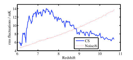
Figure 1: The rms fluctuation in differential brightness temperature, calculated at the resolution of LOFAR, in our simulation of the cosmological signal (CS) is shown as a function of redshift (solid line). For comparison, we show the rms noise for an observing time of 600 hours per frequency channel, scaled down by a factor of 6 (dotted line). Note that the vertical axis scale does not start at zero.

This rms is calculated at the resolution of LOFAR, which will be around $4\ \mathrm{arcmin}$ for EoR observations, depending on frequency. Note that the rms fluctuation does not drop to zero by the lowest redshift in this simulation, indicating that reionization is not complete there. This delay in reionization comes about because the source properties are the same as for our earlier, higher-resolution simulations, which contain more resolved haloes (i.e. the minimum resolved halo mass is lower). The larger simulations therefore have fewer sources per unit volume. Such late reionization appears unrealistic given current observational constraints (e.g.  Fan, Carilli & Keating, 2006, and references therein), and means that extracting the power spectrum at low redshift may be more difficult in reality than we would predict using these simulations. The most stringent test of our power spectrum extraction occurs at higher redshift, however, since this corresponds to lower observing frequencies at which the noise (shown in Fig. 1) and the foregrounds are larger. The power spectrum evolves less strongly at high redshift, and so we expect this simulation to perform reasonably well there compared to high resolution simulations. It may even be slightly conservative, since Hii regions at high redshift may increase the strength of fluctuations at some scales.

We use the foreground simulations of Jelić et al. (2008). These incorporate contributions from Galactic diffuse synchrotron and free-free emission, and supernova remnants. They also include unresolved extragalactic foregrounds from radio galaxies and radio clusters. We assume, however, that point sources bright enough to be distinguished from the background, either within the field of view or outside it, have been removed perfectly from the data. Observations of foregrounds at $150\ \mathrm{MHz}$ at low latitude (Bernardi et al., 2009) indicate that these simulations fairly describe the properties of the diffuse foregrounds.

2.2 Instrumental response

LOFAR is a radio interferometer which is planned to have fields of antennas (stations) in several European countries. Its core, however, is near the village of Exloo in the Netherlands, and it is the stations in the core area (and perhaps some nearby ‘remote stations’) which will be used for EoR observations. Each station contains two types of antenna: low-band antennas (LBA), optimized for $30$–$80\ \mathrm{MHz}$, and high-band antennas (HBA) optimized for $120$–$240\ \mathrm{MHz}$. The LBAs will not be sensitive enough for redshifted 21-cm work, so we will be concerned only with the HBAs. EoR observations are expected to take place below approximately $190\ \mathrm{MHz}$ (above $z=6.48$).

To improve the uv coverage (at the expense of increasing the workload of the supercomputer which acts as LOFAR’s correlator), within each LOFAR core station the HBA antennas are distributed into two semi-stations, each of which is then treated is an independent station. The antennas are collected into tiles, each of which is a grid of $4\times 4$ dual dipoles. A semi-station consists of 24 such tiles, arranged in a filled circle. A remote station has all 48 of its HBA tiles collected into a single circle. Each pair of stations provides us with one baseline.

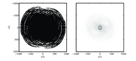
Figure 2: Assumed uv coverage at $150\ \mathrm{MHz}$ (left panel): black cells are those containing at least one observation, i.e. those having $S(u,v)>0$. The right panel shows the density of points in the uv plane, on a linear greyscale.

To include the effects of the instrumental response of LOFAR we define a sampling function $S(u,v)$ which describes how densely the interferometer baselines sample Fourier space over the course of an observation, such that $1/\sqrt{S}$ is proportional to the noise on the measurement of the Fourier transform of the sky in each uv cell. In general this sampling function is frequency-dependent, but we examine the effect of this dependence by comparing to a situation in which we assume the uv coverage is the same at all frequencies. This situation could be approximated in practice by not using data at uv points for which there is no coverage at some frequencies. This would involve discarding approximately 20 per cent of the data (from the outer part of the uv plane at high frequencies, and from the inner part at low frequencies), increasing the level of noise and reducing the resolution at high frequencies. Throughout this paper, $S(u,v)$ is computed under the assumption that 24 dual stations in the core and the first ring of LOFAR are used to observe a window at a declination of $90\degr$. We assume noise levels appropriate to an observation at the zenith, however. The final LOFAR layout is likely to include fewer dual stations, and EoR observations will use some of the more central remote stations, but we will not investigate different configurations in this paper. The sampling function and uv coverage at $150\ \mathrm{MHz}$, at which the frequency-dependent and frequency-independent sampling functions match, are shown in Fig. 2. The uv tracks are for a four-hour observation. We summarize some of the parameters of our simulated observations using this array layout in Table 1.

Table 1: Parameters of our synthetic observations and assumed array layout.

Total effective area at $150\ \mathrm{MHz}$	$2.46\times 10^{4}\ \mathrm{m}^{2}$
Image noise for a 300 hour observation	$78\ \mathrm{mK}$
with $1\ \mathrm{MHz}$ bandwidth at $150\ \mathrm{MHz}$
Frequency coverage	$121.5$–$200\ \mathrm{MHz}$
Frequency channel width	$0.5\ \mathrm{MHz}$
Station beam field of view	$5\degr\times 5\degr$
Number of instantaneous baselines	$48\times 47$
Spatial resolution at $150\ \mathrm{MHz}$	$\approx 4\ \mathrm{arcmin}$

To simulate our data in the uv plane we perform a two-dimensional Fourier transform on the image of the foregrounds and signal at each frequency, and multiply by a mask (the uv coverage) which is unity at grid points in Fourier space (uv cells) where $S(u,v)>0$, and is zero elsewhere. At this point we add uncorrelated complex Gaussian noise with an rms proportional to $1/\sqrt{S}$ to the cells within the mask. We can then return to the image plane by performing an inverse two-dimensional Fourier transform at each frequency. This two-dimensional Fourier relationship between the uv and image plane only holds approximately for long integrations with a LOFAR-type array, but we use it here since it allows considerable simplification. The overall normalization of the level of noise at each frequency is chosen to match the expected rms noise of single-channel images. Part of the aim of this paper is to check the effect of different levels of noise on power spectrum extraction. For reference, we assume that 300 hours of observation of one EoR window with one synthesized beam with LOFAR will give noise with an rms of $78\ \mathrm{mK}$ on an image using $1\ \mathrm{MHz}$ bandwidth at $150\ \mathrm{MHz}$. Although this is a somewhat conservative choice, it offsets the assumption of a uniform primary beam within the field of view we are considering, since a more realistic model for the primary beam would produce a noise rms that increased towards the edge of the field of view. The level of noise varies with frequency, being related to the system temperature which we assume to be $T_{\mathrm{sys}}=140+60(\nu/300\ \mathrm{MHz})^{-2.55}\ \mathrm{K}$.

A much more detailed account of the calculation of noise levels and the effects of instrumental corruption for the LOFAR EoR project may be found in Labropoulos et al. (2009).

3 Extraction

3.1 The problem of extraction

In this paper, the main limitation on the quality of power spectrum extraction which we will consider is the subtraction of astrophysical foregrounds. One difficulty encountered in this subtraction is simply that the fluctuations in the foregrounds are much larger than those in the CS: a subtraction algorithm must ensure that features due to the signal are not mistaken for relatively tiny features in the foregrounds. A second difficulty is the presence of noise, which limits the accuracy and precision with which we are able to measure the foregrounds, and hence the accuracy with which we can subtract them. The relative importance of these two effects changes with scale, since the power spectra of the foregrounds, signal and noise do not have the same shape.

Our foreground subtraction relies on the foregrounds being spectrally smooth, i.e. lacking small-scale features in the frequency direction. Any small-scale features are put down to noise or signal. Large-scale features due to the CS are more difficult to recover, since they can easily be confused with foreground features. The difficulty of recovering the large-scale power is exacerbated because the fluctuations in the foregrounds become larger compared to the noise and the signal, making the problem of overfitting more severe.

At small scales, the noise is more of an issue: its power spectrum becomes much larger compared to the foregrounds and signal, making the latter impossible to pick out. The scale-dependence of the contaminants means that there is a ‘sweet spot’: a range of scales at which both the foregrounds and the noise are small enough relative to the CS for the prospects for signal extraction to be good.

This fact has implications for choosing an observational strategy for the LOFAR EoR experiment, because we must trade off the depth of observation against sky and frequency coverage. A deep observation of a small area allows foreground fits of higher quality, and is especially beneficial for the recovery of small-scale power. It limits the size and number of modes which we can sample, however, which is especially damaging for the errors on the recovered large-scale power. Conversely, increasing the size of the area surveyed beats down sample variance and may allow us to probe larger scales, though note that in the case of radio interferometry the length of the shortest baselines sets an upper limit on the size of the available modes. This increase in area is only useful, however, if the noise levels are low enough to allow foreground fitting to take place.

Examining this trade-off is one of the aims of this work. Before doing so, we first outline the procedures we have used to fit the foregrounds.

3.2 Fitting procedure

As we mentioned in Section 2, we consider both the case in which the uv coverage of the observations depends on observing frequency, and the idealized case in which it does not. For the latter, we always fit the foregrounds in the image-space frequency cube using the Wp smoothing method (Mächler, 1993, 1995) described in detail in Harker et al. (2009b) and summarized in Section 3.2.1. This method requires the specification of a parameter, $\lambda$, which governs the level of regularization: larger values impose a smoother solution. We use $\lambda=0.5$ for our image-space fitting, since we found this to work well for extracting the rms (Harker et al., 2009b). Before fitting, we reduce the resolution of the images, combining blocks of $4\times 4$ pixels together to generate a $64\times 64\times 158$ data cube. Since the unbinned pixels are smaller than a resolution element of LOFAR (the binned pixels are slightly larger), and since the relative contribution of the noise increases at small scales, this does not discard spatial scales at which we can usefully extract information, but does increase the quality of the fit, reducing bias.

When the uv coverage is frequency-dependent, however, fitting in image space becomes problematic, since spatial fluctuations are converted to fluctuations in the frequency direction, as illustrated by, for example, Bowman, Morales & Hewitt (2009) and Liu et al. (2009). Instead, we leave the data cube in Fourier space [or, to be more precise, $(u,v,\nu)$-space, since we do not transform along the frequency direction], and fit the foregrounds as a function of frequency at each uv point before subtracting them and generating images. The real and imaginary parts are fit separately, using inverse-variance weights to take account of the fact that the noise properties change as a function of frequency. This implies that if a point in the uv plane is not sampled at a particular frequency, then it has zero weight and does not contribute to the fit. This is therefore similar to the method proposed by Liu et al. (2009). We discard ‘lines of sight’ in Fourier space in which the weight is non-zero for fewer than ten points, since the foregrounds are not well constrained here and we would merely introduce noise into the residual images.

This leaves the problem of which method to use to perform the fitting in Fourier space. Choosing a method is more awkward than in image space, since the mean contribution from foregrounds, noise and signal varies across the uv plane. It may be optimal to vary the parameters of a fitting method according to the position in the uv plane. None the less, we obtain reasonable results simply using a third-order polynomial in frequency to fit the real and imaginary parts at each point in the plane. We have also used Wp smoothing to fit the foregrounds in the uv plane. This gives us the freedom to vary the smoothing parameter, $\lambda$, across the plane. Near the origin (i.e. corresponding to large spatial scales) little regularization is required, since the contribution from the foregrounds is much larger than that from the signal or the noise and so they are well measured. Toward the edges of the plane we need to make stronger assumptions about the smoothness of the foregrounds to avoid overfitting, and so we make the value of $\lambda$ larger. Finding a ‘natural choice’ for $\lambda$ is somewhat awkward (see Harker et al. 2009b for further discussion), so at present we choose a mean value of $\lambda$ which gives reasonable results, and vary it between lines of sight by making it inversely proportional to the mean, $\bar{c}$, of the fitting weights of points along that line of sight. Specifically, we use $\lambda(u,v)=280/\bar{c}(u,v)$, where $c(u,v,\nu_{i})=\sqrt{S(u,v,\nu_{i})}/\sigma^{\mathrm{im}}(\nu_{i})$ and $\sigma^{\mathrm{im}}(\nu_{i})$ is the rms image noise at frequency $\nu_{i}$ expressed in kelvin. Since the noise is typically a few tenths of a kelvin, and $S$ has values ranging up to around $2.5\times 10^{5}$, we end up with $\lambda\approx 15$ at the edge of the uv plane and $\lambda\approx 0.03$ near the centre, for an integration of 300 hours. The results are not sensitive to the precise normalization of $\lambda$.

3.2.1 Wp smoothing

Wp smoothing is a non-parametric fitting method which appears to be very suitable for fitting the spectrally smooth foregrounds in EoR data sets. It was developed for general cases by Mächler (1993, 1995), and we have described an algorithm for using it for fitting EoR foregrounds in a previous paper (Harker et al., 2009b). We will briefly outline its principles here.

The aim is to fit a function $f(x)$ to a series of points $\{(x_{i},y_{i})\}$ subject to a constraint on the number of inflection points in the function, and on the integrated change of curvature away from the inflection points. More precisely, define the function $h_{f}(x)$ by

$$f^{\prime\prime}(x)=s_{f}(x-w_{1})(x-w_{2})\ldots(x-w_{n_{w}})\mathrm{e}^{h_{f}(x)},$$ (2)

where $s_{f}=\pm 1$ and $w_{1},\ldots,w_{n_{w}}$ are the inflection points. The function $f$ we wish to find is that which minimizes

$$\sum_{i=1}^{n}\rho_{i}(y_{i}-f(x_{i}))+\lambda\int_{x_{1}}^{x_{n}}h_{f}^{\prime}(t)^{2}\mathrm{d}t\ ,$$ (3)

where the function $\rho_{i}$, which takes as its argument the difference $\delta=y_{i}-f(x_{i})$ between the fitting function and the data points, penalizes the fitting function if it strays too far from the data. We opt to use a least-squares fit, with $\rho_{i}(\delta)=c_{i}/(2\delta^{2})$ where $c_{i}$ is a weight. Our choice for $c_{i}$ is given above. The parameter $\lambda$ controls the relative importance of the least-squares term and the regularization term, with larger values giving heavier smoothing.

Mächler (1993, 1995) derives an ordinary differential equation and appropriate boundary conditions such that the solution is the function $f$ which we require. We solve it by discretizing it to give an algebraic system which we solve using standard methods. It is possible to perform a further minimization over the number and position of the inflection points, but we have found that solutions with no inflection points fit the EoR foregrounds well, so we do not require this extra step.

3.3 Power spectrum estimation

Once we have fit the foregrounds, we subtract the fit to leave a residual data cube which has as its components the cosmological signal, the noise and any fitting errors. We will mainly be concerned with the spherically averaged three-dimensional power spectra of the residuals and their components. These are calculated within some sub-volume of the full data cube (for example, a slice $8\ \mathrm{MHz}$ thick) by computing the power in cells and then averaging it in spherical annuli to give band-power estimates. Each cell contributes only to the annulus in which its centre lies, i.e. we ignore the fact that the cells have non-zero size. The annuli are logarithmically spaced, but because we plot the power against the mean value of $k$ for cell centres lying within an annulus, the points in figures may not be exactly logarithmically spaced. Rather than showing the raw power, in our figures we plot the quantity $\Delta^{2}(k)=\mathcal{V}k^{3}P(k)/(2\pi^{2})$ (or the analogous one- or two-dimensional quantity: see e.g. Kaiser & Peacock, 1991), where $\mathcal{V}$ is the volume. This is usually called the dimensionless power spectrum when dealing with the spectrum of overdensities, though in this case it has the dimensions of temperature squared. $\Delta^{2}(k)$ is then the contribution to the temperature fluctuations from modes in a logarithmic bin around the wavenumber $k$.

Different systematic effects are important for modes along and across the line of sight, however. For this reason we also calculate the two-dimensional power spectrum perpendicular to the line of sight (i.e. the angular power spectrum, but expressed as a function of cosmological wavenumber $k$) and the one-dimensional power spectrum along the line of sight. We estimate the two-dimensional power spectrum at a particular frequency by averaging the power in annuli. Estimates calculated from one frequency band tend to be rather noisy, so we usually average the power spectrum across several frequency bands to give a less noisy estimate. In the one-dimensional case we simply calculate the one-dimensional power spectrum for each line of sight with no additional binning (producing points linearly spaced in $k$), then average these spectra across all $64^{2}$ lines of sight [$256^{2}$ lines of sight in the case of the cubes fit in $(u,v,\nu)$ space] to give an estimate for the whole volume. Typically we consider a volume only $\sim 8\ \mathrm{MHz}$ deep, so that the CS does not evolve too much within the volume.

To see more clearly the contribution to the power spectrum of the residuals from its different components, we write the residuals in Fourier space as

$$r(\boldsymbol{k})=s(\boldsymbol{k})+n(\boldsymbol{k})+\epsilon(\boldsymbol{k})\ ,$$ (4)

where $s$ is the cosmological signal, $n$ is the noise and $\epsilon$ is the fitting error. Then the power spectrum is given by

$$P^{r}(k)={} \langle r(\boldsymbol{k})r(\boldsymbol{k})^{\ast}\rangle_{|\boldsymbol{k}|=k}$$ (5)

$$={} P^{s}(k)+P^{n}(k)+P^{\epsilon}(k)$$

$$+\langle\epsilon(\boldsymbol{k})[s(\boldsymbol{k})+n(\boldsymbol{k})]^{\ast}+[s(\boldsymbol{k})+n(\boldsymbol{k})]\epsilon(\boldsymbol{k})^{\ast}\rangle_{|\boldsymbol{k}|=k}$$ (6)

where the subscript indicates that the averaging takes place over a shell in $k$-space, and the superscripts label the power spectra of the different components. The equality on the second line follows because the signal and noise are uncorrelated so their cross-terms average to zero. We cannot assume, however, that the fitting errors are uncorrelated with the signal or noise, which gives rise to the final term in angle brackets, which may be either positive or negative. We may usually expect it to be negative, since we fit away some of the signal and noise, reducing the size of the residuals. If it is large enough, the power spectrum of the residuals may even fall below the power spectrum of the input CS, especially at scales where the noise power is small.

If we ignore the fitting errors, we may estimate the power spectrum of the CS by computing the power spectrum of the residuals, then subtracting the expected power spectrum of the noise. In this case, we can make a relatively straightforward estimate of the error on the extracted power spectrum, as we see in Section 3.3.1. We have assumed here that the expected power spectrum of the noise is known to reasonable accuracy. In fact, we will not be able compute it accurately enough a priori for real LOFAR data: it must instead be estimated through observation. It should be possible to do so by differencing adjacent, narrow frequency channels (much narrower than those in the simulations used here, where the data have been binned into $0.5\ \mathrm{MHz}$ channels: the estimate would have to be carried out before this level of binning, using channels of perhaps $10\ \mathrm{kHz}$). Studying this in more detail in the context of the LOFAR EoR experiment must be the subject of future work, though note that this approach has already been applied to characterize the noise in low frequency foreground observations made with the Westerbork telescope (Bernardi et al., 2010), the GMRT (Ali, Bharadwaj & Chengalur, 2008) and PAPER (Parsons et al., 2009).

3.3.1 Statistical errors

The statistical errors on the extracted power spectrum include contributions from the noise and from sample variance. Considering first the noise, in the $i^{\mathrm{th}}$ Fourier cell the real and imaginary parts of the contribution to the gridded visibility from the noise, $V^{n}_{i}$, are Gaussian-distributed, with mean zero and variance $\sigma_{i}^{2}$ (say), which is known. Then $|V^{n}_{i}|^{2}$ is exponentially distributed with mean $2\sigma_{i}^{2}$ and variance $4\sigma_{i}^{4}$. We may estimate the power spectrum at some wavenumber $k$ by computing

$$\langle P^{n}(k)\rangle=\frac{1}{m_{k}}\sum_{i=1}^{m_{k}}|V^{n}_{i}|^{2}$$ (7)

where the sum is over all cells within an annulus near $k$. If the number of cells in the annulus is sufficiently large, the error on this estimate is approximately Gaussian-distributed, and we estimate it as $\langle P^{n}(k)\rangle/\sqrt{m_{k}}$, assuming that the different cells are independent and using the fact that the variance of $|V^{n}_{i}|^{2}$ is the square of its mean. This error translates into an error on the final extracted power spectrum, and can be reduced either by integrating longer on the same patch of sky (to reduce $\sigma_{i}^{2}\sim 1/\tau$ where $\tau$ is the observing time) or by spending the time observing a wider area to increase the number of accessible modes, increasing $m_{k}$. In the latter case, the error only decreases as $1/\sqrt{\tau}$.

Though this estimate of the error is useful as a guide for how the errors behave as the observational parameters change, a more accurate error bar can be computed in a Monte Carlo fashion by looking at the dispersion between independent realizations of the noise, and this is how we compute the errors in practice. Although the analytic estimate is reasonable, it tends to underestimate the errors at large scales and overestimate them at small scales.

The power spectrum of our simulation of the CS is calculated similarly to the power spectrum of the noise. In this case, the error $\langle P^{\mathrm{CS}}(k)\rangle/\sqrt{m_{k}}$ represents the error on our final estimate of the power spectrum due to sample variance, and can only be reduced by sampling more modes (increasing $m_{k}$). Unlike the noise, the fluctuations in the CS are not Gaussian, and so an analytic estimate of the error is likely to be less accurate. This should not matter too much at small scales where in any case the error on our extracted power spectrum is dominated by noise, but on larger scales the sample variance becomes important. At present we do not have enough different realizations of the CS to simulate the errors more realistically: as noted in Section 2 we must already tile copies of a single simulation to fill a LOFAR field of view, which limits the range of scales we can realistically study. These estimates should therefore be considered an illustration of how we expect the errors to change as we vary our observational strategy, rather than a definitive calculation, which is reasonable given the other simplifications we have made (e.g. adopting a square field of view rather than a realistic primary beam shape). Error bars on our extracted power spectra are computed by adding the noise and sample variance errors in quadrature.

3.3.2 Systematic errors

The terms involving fitting errors on the right-hand side of equation (6) will bias our estimate of the power spectrum of the CS unless they can be accurately corrected for, and so contribute to a systematic error. When analysing LOFAR data it may be possible to estimate the size of these terms using simulations similar to the ones used in this paper. Bowman et al. (2009) have estimated them for simulations of MWA data through a ‘subtraction characterization factor’ $f_{s}(k)=\langle P^{s}(k)\rangle/P^{s}(k)$. By fitting cubes which include different realizations of the CS and noise, it should also be possible to reflect the statistical error introduced by making such a correction in the error bars. In this paper we do not make this correction, however: it would be accurate by construction and hence quite uninformative. Instead we plot $\langle P^{s}(k)\rangle=P^{r}(k)-\langle P^{n}(k)\rangle$ to illustrate the level of bias we may expect to see if no correction is made. Our error bars will then reflect errors due only to the sample variance and the noise. If the estimated power falls below the true power, we use the estimate of sample variance from the true power, since this gives a more realistic view of what the estimate of the sample variance would be if we made a correction for the fitting bias.

We expect any estimate of the bias, or of the statistical error introduced by correcting for the bias, to be rather uncertain, since it may depend strongly on the shape of the foregrounds, which is unknown to the required level of accuracy a priori, and on the details of the fitting procedure used. It is none the less straightforward to estimate them for a specific foreground model and fitting procedure.

3.3.3 Cross-correlation

As an alternative to calculating a residual power spectrum and then subtracting a thermal noise power spectrum, we could obtain the extracted power spectrum through cross-correlation. That is, we could split an observing period into two sub-epochs, subtract the foregrounds from each and then cross-correlate the two. Following the approach taken to derive Equation (6), we can write the residual in each of the two epochs as

$$r_{i}(\boldsymbol{k})=s(\boldsymbol{k})+n_{i}(\boldsymbol{k})+\epsilon_{i}(\boldsymbol{k})\ ,$$ (8)

where the signal $s(k)$ is the same for the two cases and $i\in\{1,2\}$ labels the epoch. Then

$$\langle r_{1}r_{2}^{\ast}\rangle=P^{s}+\langle s\epsilon_{2}^{\ast}\rangle+\langle\epsilon_{1}s^{\ast}\rangle+\langle\epsilon_{1}\epsilon_{2}^{\ast}\rangle\ ,$$ (9)

where the $\boldsymbol{k}$-dependence is implicit, the angle brackets again indicate an average over a shell in $k$-space, and cross-terms involving the noise vanish. If the fitting errors are sufficiently small, this cross-correlation immediately provides us with an estimate of the desired power spectrum.

This estimator has some apparent advantages. Firstly, we do not have to know the thermal noise power spectrum to calculate it (though an estimate of the thermal noise is required to compute error bars). Secondly, we do not expect it to yield negative estimates of the power, as may happen when using Equation (6). More generally, at scales where the noise is larger than the signal or the fitting errors, we would expect the bias of this estimator to be much smaller than for the one involving autocorrelations, since the cross-terms involving $n$ and $\epsilon$ on the right-hand side of Equation (6) do not appear.

It is not without disadvantages, however. If we split the observation into two epochs, the lower signal-to-noise in each epoch will degrade the foreground fitting, increasing the size of the $\epsilon$ terms. If, instead, the foreground fitting is done on the full dataset before dividing it into different epochs, then the cross-terms involving $n$ and $\epsilon$ can no longer be assumed to vanish.

We have conducted preliminary tests of the cross-correlation method and found that it gives comparable results to the autocorrelation method at scales where the fitting bias is small enough for either estimate to be useful. We reiterate, however, that it is assumed here that the thermal noise power spectrum is known accurately, which unfairly favours using the autocorrelation. We defer further comparison of the two methods until we have looked further into how well the noise power spectrum can be estimated from observations. In this paper, all our extracted power spectra are computed by subtracting the noise power spectrum from the residual power spectrum. We would not expect our broad conclusions to change if we were to use cross-correlation instead.

4 Sensitivity estimates

4.1 Comparison of fitting methods

Examples of extracted power spectra at three different redshifts, for slices $8\ \mathrm{MHz}$ thick, are given in Fig. 3 (points with error bars).

Figure 3: Power spectra of the input CS (solid line), the noise (dashed line), the residuals (dotted line) and the extracted signal (points with error bars) at three different redshifts. Here we assume the uv coverage is frequency-independent, so the foreground fitting is done using Wp smoothing in the image plane. The noise level is consistent with 300 hours of observation per frequency bin on a single window, using one station beam. The redshift shown in each panel is the central redshift of an $8\ \mathrm{MHz}$ slice from the frequency cube. This frequency interval corresponds to $\Delta z=0.63$, $0.48$ and $0.37$ for the top, middle and bottom panel respectively. From top to bottom, the mean neutral fraction in each slice, $\bar{x}_{\mathrm{HI}}$, is 0.9976, 0.9416 and 0.6140. The missing points in the top panel correspond to $k$ bins at which the power spectrum of the residuals falls below the power spectrum of the noise, so that we would infer an unphysical, negative signal power.

From top to bottom, the central redshift of the slice used in each panel is 9.96, 8.49 and 7.37, while the mean neutral fraction $\bar{x}_{\mathrm{HI}}$ in each slice is 0.998, 0.942 and 0.614, respectively.

For comparison, we also show the power spectrum of the noiseless CS cube (solid line), the noise (dashed line) and the residuals after fitting (dotted line). The extracted power spectrum is the difference between the residual and noise power spectra, and would be equal to the noiseless CS power spectrum if there were no foregrounds. For this figure we use a frequency-independent uv coverage, so the foreground fitting is carried out in the low-resolution image cube. A noise level consistent with 300 hours of observation per frequency bin of a single ($5\degr\times 5\degr$) window using a single station beam is assumed. It may not be possible to observe the entire frequency range simultaneously, and it may have to be split into two or three segments (e.g. of $32\ \mathrm{MHz}$ width) only one of which can be observed at once. If we have to use two such segments, then the 300 hours of observation per frequency bin translates to 600 hours of total observing time. This is a somewhat pessimistic scenario for the quality of data we may collect after one year of EoR observations with LOFAR, since it is hoped that several station beams can be correlated simultaneously to cover the top of the primary (tile) beam, allowing a larger field of view to be mapped out more quickly. It may also be possible to trade off the number of beams against the width of the frequency window, or to spend different amounts of time on different parts of the frequency range. None the less, the assumptions of Fig. 3 provide a useful baseline against which we can compare results for deeper observations or for more realistic (frequency-dependent) uv coverage. It also illustrates the main features we see in many of our extracted spectra.

For the lowest-redshift slice (bottom panel), the recovery appears to be good: at most scales, the recovery is accurate and has small errors. At large scales the error bars increase in size because of sample variance, and it appears that the recovered power spectrum lies systematically below the input spectrum. This happens because at large scales, we fit away some of the signal power during the foreground fitting. If the points at large scales do not appear to jump around as one would expect given the size of the error bars, this is because the error bars here are dominated by sample variance, and so show our uncertainty as to how representative this volume is of the whole Universe. If, instead, we showed error bars showing only the uncertainty on our determination of the power spectrum within this volume, they would be much smaller and would be visually consistent with the scatter displayed by the points. The error bars grow at small scales because the noise power becomes larger compared to the signal power, limiting our sensitivity. We caution that, as noted in Section 2, the simulation we use represents a rather optimistic scenario for low-redshift signal extraction, since reionization occurs very late.

As we move to higher redshift (middle panel) the situation worsens slightly, with the error bars increasing in size because of the higher noise levels. More worryingly, the recovered power is lower than the input power at all scales (though it becomes worse at large scales as before) which seems to indicate that foreground subtraction may cause significant bias in our estimate of the signal power even at intermediate scales. The trend continues as we move to the highest redshift slice (top panel). We do not plot the recovered power for a range of scales between $k\approx 10^{-0.9}$ and $10^{-0.3}\ h\ \mathrm{Mpc}^{-1}$. This is because we infer an unphysical negative power here. In the case of such points we plot a statistical upper limit on the power. The bias from the fitting procedure leads to a situation where these ‘upper limits’ lie below the true power, or are too small even to show up on the plot. These upper limits should, then, be taken merely as an indication of the size of the fitting bias. The larger noise at lower frequencies (higher redshifts) increases the size of the error bars compared to the other panels. The combination of this higher noise and the larger foreground power makes fitting the foregrounds at high redshift more difficult, as we have seen in previous work (Harker et al., 2009a, b), leading to the observed bias.

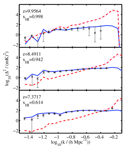
Figure 4: Power spectra of the CS, the noise, the residuals and the extracted signal for the case when the uv coverage is frequency-dependent, we have 300 hours of observation per frequency channel with a single station beam, and the foreground fitting is done using Wp smoothing in Fourier space. The redshift slices and the colour coding of the lines are the same as for Fig. 3, but note we have changed the scale of the vertical axis to accommodate the upturn in noise power at small scales.

The situation is very similar if the uv coverage is frequency-dependent but we do our fitting using Wp smoothing in Fourier space. This case can be seen in Fig. 4, which is otherwise very similar to Fig. 3 except that we have changed the vertical axis scale to accommodate the upturn in noise power at high $k$ caused by the varying uv coverage. The higher small-scale noise coming from the frequency-dependent uv coverage damages the recovery of power at the smallest scales, but the fitting using Wp smoothing in Fourier space allows us to recover the power on intermediate and large scales even better than in Fig. 3. The reason that we fit even better than in the supposedly more ideal case of Fig. 3 is partly that the noise is normalized in image space to the expected level for single-channel images (see Section 2.2), and so the increase in small-scale noise in the frequency-independent case is compensated by a reduction in large-scale noise, improving recovery there. It is also the case that our uv plane fitting is more adaptive, applying less regularization at scales where the foregrounds dominate and the noise is low. Unfortunately we do not yet have a well-motivated method to choose the regularization parameter $\lambda$ automatically rather than varying it by hand, but this result suggests that finding a suitable method could yield even more improvement in the quality of the fitting.

If we use a third-order polynomial fit for the foregrounds rather than using Wp smoothing, however, the result becomes worse, especially at high redshift. This is illustrated in Fig. 5, which is identical to Fig. 4 apart from the fact that polynomial fits are used.

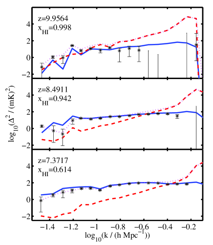
Figure 5: As for Fig. 4, except that the foregrounds are fit using a third-order polynomial rather than Wp smoothing.

While at low redshift the quality of recovery is visually indistinguishable, at high redshift the Wp smoothing of Fig. 4 allows us to recover an estimate of the power spectrum to higher $k$. The bias at low $k$ also seems to be larger for polynomial fitting, which seems to produce overestimates of the power of the CS at large scales. This may be due to the fact that a polynomial is unable to match the large-scale spectral shape of the foregrounds, allowing foreground power to leak into the residuals. Unlike Wp smoothing, polynomial fitting does not allow us to smoothly vary the level of regularization across the uv plane (the only parameter we can tweak is the polynomial order, which is a somewhat blunt instrument) and this may also contribute to the poorer fit.

We conclude that even though varying uv coverage makes foreground fitting more awkward, we can mitigate its effects without having to discard a large proportion of our data if we choose our fitting method carefully. At present our scheme for fitting the foregrounds using Wp smoothing in Fourier space is quite slow, however, so for the rest of the paper we revert to the case of frequency-independent uv coverage, for which our image-space fitting works quickly and reasonably well. Fig. 4 suggests that this should not affect our comparisons of results using different lengths of observing time or observational strategies. For actual LOFAR data, the fitting of the foregrounds should still be much faster than other steps in the reprocessing of the data, and so we are likely to use our most accurate scheme (at present, Wp smoothing in Fourier space) even if it is slow compared to other schemes.

4.2 Different depths and strategies

Having compared the characteristics of different fitting methods, we now move on to comparing the quality of extraction for different assumptions about the amount of observing time, and for different observational strategies. We start by showing the extraction for 180 hours of observing time per frequency bin, making a total of 360 hours of observing time if two frequency ranges are required, in Fig. 6.

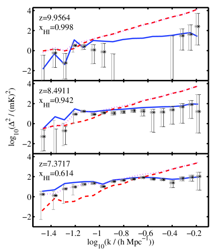
Figure 6: As for Fig. 3, but using a noise level consistent with 180 hours of observation per frequency bin on a single window, using one station beam. We also plot two error bars for each point: the grey one on the left shows the error from both noise and sample variance as in our other figures, while the black one on the right shows the error only from noise.

This makes it comparable to fig. 12 of Bowman et al. (2009), who show a simulated power spectrum for 360 hours of observation with the MWA (though spanning a larger redshift range than a panel of our figure). To make the comparison more illustrative, we show two error bars for each point, the grey one on the left including both the noise error and the sample variance, and the black one on the right including only the noise error. For the MWA these would differ by less then ten per cent and would be almost indistinguishable on this log-log scale (J. Bowman, private communication). Visually, the errors for LOFAR without sample variance appear smaller than those for the MWA at most scales at the lower redshifts, as we may expect from the larger collecting area. A computation including the sample variance, however, tends to favour the MWA at small $k$ owing to its larger field of view. Hence we explore the effect of observing multiple independent windows below.

The field of view can also be extended if, as planned, we are able to synthesize multiple station beams simultaneously. Equivalently, if we wish from the outset to observe a window larger than the $\sim 5\degr\times 5\degr$ of a single station beam, multiple beams can be used to achieve observations of greater depth without using more observing time. We show the effect of extending the field of view in Fig. 7, where we assume that we observe for 300 hours per frequency bin (as in Fig. 3), but using six station beams.

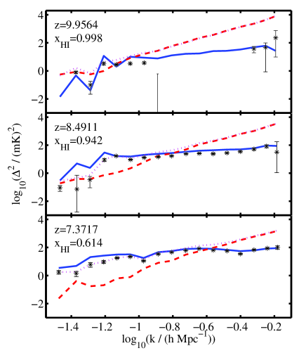
Figure 7: As for Fig. 3, except we assume that six station beams are synthesized, rather than one.

We model the effect of using six beams by reducing the errors due to noise and to sample variance by a factor of $\sqrt{6}$. A realistic primary beam model, and the incorporation of modes with smaller $k$, would make the effect of multiple beams more complicated, but we incorporate the effect in a way which is consistent with our simplified beam. The most obvious effect of using multiple beams is at large scales, since here the increase in the number of available modes reduces the (large) sample variance errors as well as the noise errors. The noise errors at high $k$ are also reduced, however. Since the smallest scales we probe may be comparable to the size of bubbles in the HI distribution, this improvement may be important for constraining physical models.

This figure also makes it clear what multiple beams do not do. Increasing the field of view in this way does not increase the signal to noise along each line of sight, and so the foreground fitting does not improve. The systematic offset at intermediate scales in the middle redshift bin is still present, and we remain unable to extract physically meaningful information at high redshifts at these scales with our current methods. Our CS simulations are of limited size, so we are unable to demonstrate how the larger field of view enables us to recover the power spectrum at lower $k$. The bias we see at the largest scales in our figures is unlikely to improve as we go to yet larger scales, however, and so it may be difficult to exploit the potential afforded by a larger field of view in practice.

We now directly examine the trade-off between spending observing time to go deeper in a small area, and spending it to survey a larger area. Considering first the situation at the lowest redshifts, we see from Figs. 6 and 7 that after 180 hours of observation per frequency channel, the fitting bias has reached a level that reduces very little with deeper observation. Moreover, with the six station beams of Fig. 7 the errors at intermediate scales are rather small. The main effect of deeper observation is then to reduce the errors only at the very smallest scales. It would clearly be more profitable to use extra observing time to cover multiple windows, and reduce the large-scale errors which are dominated by sample variance.

At high redshift the trade-off between depth and number of windows is more interesting, as we see in Fig. 8.

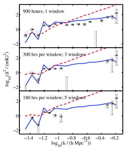
Figure 8: Power spectra of the original and extracted signal, the residuals and the noise, using the same line styles as Fig. 3. Each panel assumes the same total observing time (900 hours) using six station beams, in an $8\ \mathrm{MHz}$ slice centred at $z=9.96$ (with $\bar{x}_{\mathrm{HI}}=0.9976$), the same redshift as for the top panel of Figs. 3–7. The panels differ in the way in which the observing time is split between windows: in the top panel we devote all the observing time to a single window, and in the bottom panel we spread it equally between five different windows. The middle panel shows an intermediate case. Each point has two error bars, the one on the right accounting only for noise, and the one on the left also including the effect of sample variance, as in Fig. 6.

Here, all three panels show power spectra at the same redshift as the top panel of our earlier figures ($z=9.9564$, with $\bar{x}_{\mathrm{HI}}=0.9976$). Each point has two error bars, the one on the right accounting only for noise, and the one on the left also including the effect of sample variance, as in Fig. 6. The different panels distinguish between different ways of allocating a fixed amount (900 hours) of observing time per frequency band with six station beams. If we use this time to observe five different windows (bottom panel), as seems to be preferable at low redshift, the main effect is to reduce the size of the statistical errors in a region of the power spectrum (low $k$) where there is in any case a relatively large and uncertain systematic correction to be made for the fitting bias. Meanwhile, the large amount of noise per window degrades the fitting at intermediate scales. Taking 300 hours of observation per frequency band per window (middle panel) reduces the bias somewhat, and enables recovery of reasonable quality across a larger range of scales. Only with 900 hours of observation of a single window (top panel), however, are we able to recover a physically plausible estimate of the power across almost all the accessible scales. Even at those scales at which the shallower observations allowed some sort of estimate of the power, the increased depth reduces the bias from the fitting, so that it becomes comparable to the statistical error bars.

The tension between optimizing low- and high-redshift recovery is not the only consideration in deciding how many windows to observe and for how long. Using multiple windows will help to control the systematics because we can then compare fields with different foregrounds and different positions in the sky. If we wish to observe for a reasonable fraction of the year, we are required to observe different windows since some may be inaccessible or too low in the sky during some periods. None the less, a hybrid strategy in which some windows receive more time than others may be possible.

Another possible strategy, since the higher redshift bins appear to benefit more from longer integration times, is to spend longer observing higher redshifts than lower redshifts. Since we already split up the frequency range into different chunks which are not observed simultaneously, this may be possible without excessive difficulty. We note, however, that for other reasons (for example improving the calibration), it may be desirable not to split the frequency range into large contiguous chunks, but into two interleaved combs. This would enforce a uniform integration time across the whole frequency range. A further problem one may envisage is that the noise rms would jump discontinuously across the gap between the two frequency chunks. Unless the noise is well characterized, such a jump could be confused with a change in the signal rms due to reionization. It may also complicate the foreground fitting, and so we test this in Fig. 9.

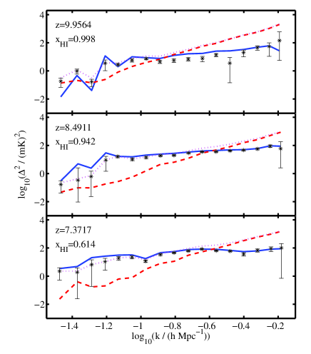
Figure 9: Power spectra at three different redshifts, using the same line styles as before. In this case, however, we assume that at frequencies above $160\ \mathrm{MHz}$ (corresponding to $z\approx 7.9$) we have used 300 hours of integration time, while below $160\ \mathrm{MHz}$ we have used 1200 hours of integration time, in each case using one station beam.

Here we have assumed that we have spent 1200 hours on the low frequency chunk (below $160\ \mathrm{MHz}$), and only 300 hours on the high frequency chunk. This does not appear to affect our fitting adversely. Even if we choose to plot the power spectrum in an $8\ \mathrm{MHz}$ slice which straddles the crossover between long and short integration times, the extraction appears to be stable. If other factors allow us to use such a strategy, then, it appears to be a viable way to make the quality of our signal extraction more uniform across the redshift range we probe.

4.3 Source of the large-scale bias

Even when we achieve small statistical errors, as for the bottom panel of Fig. 7, a bias persists on large scales. We look for the origin of this bias by plotting the power spectrum of modes in the plane of the sky (the angular power spectrum) in Fig. 10, and the one-dimensional power spectrum along the line of sight in Fig. 11. For both of these figures we consider a slice at low redshift (as for the bottom panel Fig. 7), and assume 900 hours of observation per frequency chunk with one station beam.

The extracted two-dimensional power spectrum appears to behave similarly to the three-dimensional power spectrum, albeit with slightly larger error bars because we have fewer modes available. The bias at large scales persists: we underestimate the power because we fit away some of the signal and noise. The one-dimensional power spectrum looks rather different. It is quite accurately determined because we average over so many lines of sight, and there is no apparent bias in the extraction. The one-dimensional power spectrum does not extend to such large scales as the two-dimensional power spectrum because we restrict ourselves to quite a narrow frequency slice (corresponding to a comoving depth of $93.2\ h^{-1}\ \mathrm{Mpc}$) to avoid evolution effects, but it does extend to scales at which the two-dimensional power spectrum shows bias. We have experimented with using slices which are twice as thick ($16\ \mathrm{MHz}$) and these still show no significant bias at the largest scales. The one-dimensional power spectrum extends to smaller scales than the two-dimensional one, since the spatial resolution is better along the frequency direction for our $0.5\ \mathrm{MHz}$ channels. This resolution, and the lack of bias, may be useful if we are able to invert the one-dimensional power spectrum to recover the three-dimensional power spectrum (Kaiser & Peacock, 1991; Zaroubi et al., 2006).

At first sight it seems somewhat puzzling that although we assume that the foregrounds are smooth in the frequency direction – we effectively ignore very large-scale power along the line of sight – the fitting bias manifests itself most clearly in the angular power spectrum. Note, though, that if our estimate of the foregrounds along a line of sight is offset by some constant, or by an amount that is approximately constant within the narrow frequency range in which we estimate the power spectrum (the fits are always computed across the full frequency range to avoid edge effects), this does not change the power spectrum of the residuals along the line of sight at all. If this offset is different between different lines of sight, though, then this will be apparent in the angular power spectrum of the residuals at each frequency. If the offsets at nearby points are correlated, perhaps because the foregrounds within some region have a similar shape and strength, then the angular power spectrum of the residuals on small scales will hardly be affected. At scales larger than the correlation length of the fitting errors then these offsets could lead to the bias which we see.

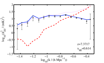
Figure 10: Two-dimensional power spectrum in the plane of the sky, for a slice $8\ \mathrm{MHz}$ thick centred at $z=7.3717$ and with $\bar{x}_{\mathrm{HI}}=0.6140$, for 900 hours of integration with a single station beam. The line styles for the original signal, noise, residuals and extracted spectrum are as for the previous figures.

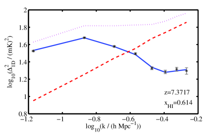
Figure 11: One-dimensional power spectrum along the line of sight, for a slice $8\ \mathrm{MHz}$ ($93.2\ h^{-1}\ \mathrm{Mpc}$) deep centred at $z=7.3717$ and with $\bar{x}_{\mathrm{HI}}=0.6140$, for 900 hours of integration with a single station beam. The line styles for the original signal, noise, residuals and extracted spectrum are as for the previous figures.

In any case, Figs. 10 and 11 suggest that we should consider the angular and line-of-sight power spectra separately in an analysis of LOFAR data, though ultimately neither will allow us to constrain models as tightly as a three-dimensional power spectrum which includes a contribution from all modes. The line-of-sight power spectrum appears to be less vulnerable to bias and extends to higher $k$, while the angular power spectrum extends to larger scales and may have greater power to distinguish between models of reionization. The more sophisticated version of this separation – expanding the three-dimensional power spectrum $P(k,\mu)$ in powers of $\mu$, the cosine of the angle between a mode and the line-of-sight (Barkana & Loeb, 2005) – is, unfortunately, not likely to be useful for the noise levels expected for LOFAR, though we have not yet made a quantitative investigation of this possibility. Pritchard & Loeb (2008) have checked this for an MWA-type experiment, using an optimistic instrumental configuration, and find that it does not have the required sensitivity. Rather, the separation into powers of $\mu$ may have to wait for SKA or for a futuristic lunar array.

5 Summary and discussion

In this paper we have studied the extraction of the 21-cm EoR power spectrum from simulated LOFAR data. The simulations allow us to compute the statistical errors on the power spectrum due to thermal noise and sample variance, and these are small enough to raise the possibility of a significant detection of emission from the EoR using only a modest amount of observing time. If we wish to estimate the power spectrum accurately, however, this becomes more challenging once we take into account the presence of fitting errors from the subtraction of astrophysical foregrounds. These errors are correlated (positively or negatively) with the signal and the noise in general, and introduce a scale-dependent bias into our estimate of the power spectrum. We anticipate that simulations such as the ones studied here could be used to estimate and correct for the bias; this would induce a further statistical error which can be straightforwardly computed by using multiple realizations of a simulated observation. Making this sort of correction will always be uncertain, though, so it is desirable to minimize its size. We have looked at the extent to which the size of the correction, as well as the size of the statistical errors, can be reduced by observing for longer or using alternative observational strategies.

Before that, though, we tested that extraction is still possible if we do not make the assumption that the uv coverage is independent of frequency. We find that this necessitates fitting the foregrounds in the $(u,v,\nu)$ cube rather than the image cube, as noted by Liu et al. (2009). The Wp smoothing method, which we have used previously to fit the foregrounds in the image cube, can be adapted to work in the $(u,v,\nu)$ cube by fitting the real and imaginary parts independently for each uv cell and by varying the regularization parameter, $\lambda$, across the uv plane. This yields results comparable to (in fact, even better than) those we obtain if we assume frequency-independent uv coverage and then fit in the image cube. We have also tried using a third-order polynomial to fit the foregrounds in the $(u,v,\nu)$ cube: this yields results which are acceptable, but not as good as those obtained using Wp smoothing. The main drawback of Wp smoothing in this case is its speed, especially for ‘lines of sight’ near the centre of the uv plane where it is best to choose a small value for $\lambda$ (implying little smoothing). Because Wp smoothing in the image cube is faster, because the polynomial fitting gives worse results than Wp smoothing in the $(u,v,\nu)$ cube, and because Wp smoothing produces extraction of similar quality in the image and $(u,v,\nu)$ cubes, we have concentrated on results using frequency-independent uv coverage to explore the different scenarios in this paper.

We have found that a year’s observations (of, say, 600 hours, of which perhaps 360 could be of a single window) should be sufficient to detect cosmological 21-cm emission from towards the end of the EoR. We caution, however, that the approximations employed in this paper prevent us from treating these numbers as more than rough estimates. If we wish to study the power spectrum at small or large scales – away from the ‘sweet spot’ at intermediate $k$ – it will be important to be able to synthesize multiple station beams. This allows us to reduce the statistical errors from sample variance and noise. Unfortunately, however, there appears to be no substitute for extending the integration time, especially to probe high redshifts and very small scales. This is because only deep observations can improve the quality of the foreground fitting, and hence reduce the systematic offset between the true signal and the recovered signal.

Under the optimistic assumptions that we can synthesize six beams, and that the useful frequency range can be covered using just two frequency bands (the instantaneous frequency coverage is limited), 600 hours of observation of a single window should be enough to yield quite precise and accurate power spectra up to $z\approx 9$, for $k$ between approximately 0.03 and $0.6\ h\ \mathrm{Mpc}^{-1}$. Pushing to the very highest redshifts accessible with the frequency coverage of LOFAR’s high band antennas requires somewhat longer: perhaps 900 hours per frequency band, which corresponds to 1800 hours of observation if there are two frequency bands.

With observations of this depth, the limiting factor in the statistical errors comes from sample variance on large scales, which can only be reduced by observing a larger area of sky. This is one of several reasons why the LOFAR EoR project plans to observe multiple – perhaps five – independent windows. We have already seen that approximately 600 hours per window is required for the thermal noise errors to be small and the bias to be under control for redshifts less than about 9. For five windows, this corresponds to 3000 hours of observation. Comparing the independent windows will also allow important cross-checks, in particular that systematics are under control.

To really push towards precise constraints on the power spectrum towards the start of reionization, the 1800 hours per window that we find yelds high quality extraction at $z>10$ corresponds to 9000 total hours for five windows. This figure may be reduced if a hybrid strategy, in which we integrate for a longer time in lower frequency bands, turns out to be feasible. From the point of view of foreground fitting and power spectrum extraction, ignoring constraints that may be imposed by calibration etc., a hybrid strategy does indeed seem to be feasible. Of course, we have considered this strategy only from the point of view of the power spectrum. If deeper observations at all frequencies would allow us to push beyond the power spectrum, perhaps into a regime where we can observe individual features in the distribution of 21-cm emission towards the end of reionization with reasonable signal to noise, then this would surely be valuable too.

Other hybrid strategies are also possible, for example ones in which different windows are observed for different amounts of time. We have not studied them here since they do not really impact the fitting and extraction, which is independent for each window. None the less, they may allow us to obtain high redshift constraints by observing one window deeply, while simultaneously allowing us to beat down sample variance errors on large scales at low redshifts by observing several other windows at reduced depth.

In any case, our study suggests that as the amount of time spent observing the EoR with LOFAR is increased, this allows us to make qualitative improvements to the fitting, and to the range of scales and redshifts we can probe accurately. Deeper integration does more than simply allow us to shrink our statistical error bars.

This all depends, however, on the robustness of our fitting techniques, and more generally on the level of control we are able to exercise over systematic errors. The Wp smoothing method we have introduced previously appears to work well when it comes to extracting the power spectrum. This holds whether we apply it to an idealized case in which the uv coverage of the instrument is constant with frequency, or to a more realistic case in which it varies. We confirm a suspicion we have expressed previously (Harker et al., 2009b) that the power spectrum may be easier to extract than an apparently simpler statistic such as the rms of the 21-cm signal: the fitting errors are scale-dependent, and a power spectrum analysis allows us to pick out the scales where our method works best without being swamped by small-scale noise. Splitting the power spectrum into angular and line-of-sight components may help us to test the robustness of our conclusions, and perhaps extend the spatial dynamic range we can probe.

We have assumed here that the power spectrum of the noise is known to reasonable accuracy, an assumption which will be examined in future work. We will also study in a future paper how different strategies alter our ability to constrain the parameters of reionization models.

Finally, we note that foreground fitting and power spectrum extraction are late steps in the collection and analysis of LOFAR EoR data. They depend on earlier and probably more difficult steps, such as instrumental calibration (including polarization, which we have neglected here), correcting for the ionosphere, and the excision of RFI. The results of this paper only reassure us that the later stages are unlikely to be the limiting ones.

References

- Ali et al. (2008) Ali S. S., Bharadwaj S., Chengalur J. N., 2008, MNRAS, 385, 2166
- Barkana (2009) Barkana R., 2009, MNRAS, 397, 1454
- Barkana & Loeb (2005) Barkana R., Loeb A., 2005, ApJL, 624, L65
- Benson et al. (2006) Benson A. J., Sugiyama N., Nusser A., Lacey C. G., 2006, MNRAS, 369, 1055
- Bernardi et al. (2009) Bernardi G. et al., 2009, A&A, 500, 965
- Bernardi et al. (2010) Bernardi G. et al., 2010, A&A, submitted
- Bowman et al. (2006) Bowman J. D., Morales M. F., Hewitt J. N., 2006, ApJ, 638, 20
- Bowman et al. (2007) Bowman J. D., Morales M. F., Hewitt J. N., 2007, ApJ, 661, 1
- Bowman et al. (2009) Bowman J. D., Morales M. F., Hewitt J. N., 2009, ApJ, 695, 183
- Ciardi & Madau (2003) Ciardi B., Madau P., 2003, ApJ, 596, 1
- Di Matteo et al. (2002) Di Matteo T., Perna R., Abel T., Rees M. J., 2002, ApJ, 564, 576
- Fan et al. (2006) Fan X., Carilli C. L., Keating B., 2006, ARA&A, 44, 415
- Field (1958) Field G. B., 1958, Proc. Inst. Radio Eng., 46, 240
- Field (1959) Field G. B., 1959, ApJ, 129, 536
- Furlanetto et al. (2006) Furlanetto S. R., Oh S. P., Briggs F. H., 2006, Physics Reports, 433, 181
- Harker et al. (2009b) Harker G. et al., 2009b, MNRAS, 397, 1138
- Harker et al. (2009a) Harker G. J. A. et al., 2009a, MNRAS, 393, 1449
- Hogan & Rees (1979) Hogan C. J., Rees M. J., 1979, MNRAS, 188, 791
- Jelić et al. (2008) Jelić V. et al., 2008, MNRAS, 389, 1319
- Kaiser & Peacock (1991) Kaiser N., Peacock J. A., 1991, ApJ, 379, 482
- Kumar et al. (1995) Kumar A., Subramanian K., Padmanabhan T., 1995, JA&AS, 16, 83
- Labropoulos et al. (2009) Labropoulos P. et al., 2009, MNRAS, submitted (arXiv:0901.3359)
- Lidz et al. (2008) Lidz A., Zahn O., McQuinn M., Zaldarriaga M., Hernquist L., 2008, ApJ, 680, 962
- Liu et al. (2009) Liu A., Tegmark M., Bowman J., Hewitt J., Zaldarriaga M., 2009, MNRAS, 398, 401
- Loeb & Barkana (2001) Loeb A., Barkana R., 2001, ARA&A, 39, 19
- Mächler (1993) Mächler M., 1993, Research report 71, Very smooth nonparametric curve estimation by penalizing change of curvature. Seminar für Statistik ETH Zürich
- Mächler (1995) Mächler M., 1995, Annals of Statistics, 23, 1496
- Madau et al. (1997) Madau P., Meiksin A., Rees M. J., 1997, ApJ, 475, 429
- Mao et al. (2008) Mao Y., Tegmark M., McQuinn M., Zaldarriaga M., Zahn O., 2008, Phys. Rev. D, 78, 023529
- McQuinn et al. (2006) McQuinn M., Zahn O., Zaldarriaga M., Hernquist L., Furlanetto S. R., 2006, ApJ, 653, 815
- Morales & Hewitt (2004) Morales M. F., Hewitt J., 2004, ApJ, 615, 7
- Oh & Mack (2003) Oh S. P., Mack K. J., 2003, MNRAS, 346, 871
- Parsons et al. (2009) Parsons A. R. et al., 2009, AJ, submitted (arXiv:0904.2334)
- Pritchard & Furlanetto (2007) Pritchard J. R., Furlanetto S. R., 2007, MNRAS, 376, 1680
- Pritchard & Loeb (2008) Pritchard J. R., Loeb A., 2008, Phys. Rev. D, 78, 103511
- Scott & Rees (1990) Scott D., Rees M. J., 1990, MNRAS, 247, 510
- Sethi & Haiman (2008) Sethi S., Haiman Z., 2008, ApJ, 673, 1
- Shaver et al. (1999) Shaver P. A., Windhorst R. A., Madau P., de Bruyn A. G., 1999, A&A, 345, 380
- Thomas & Zaroubi (2008) Thomas R. M., Zaroubi S., 2008, MNRAS, 384, 1080
- Thomas et al. (2009) Thomas R. M. et al., 2009, MNRAS, 393, 32
- Zaldarriaga et al. (2004) Zaldarriaga M., Furlanetto S. R., Hernquist L., 2004, ApJ, 608, 622
- Zaroubi et al. (2006) Zaroubi S., Viel M., Nusser A., Haehnelt M., Kim T., 2006, MNRAS, 369, 734