Parallel structurally-symmetric sparse matrix-vector products
on multi-core processors ††thanks: This work was partially supported by CNPq, Brazil.
Abstract
We consider the problem of developing an efficient multi-threaded implementation of the matrix-vector multiplication algorithm for sparse matrices with structural symmetry. Matrices are stored using the compressed sparse row-column format (CSRC), designed for profiting from the symmetric non-zero pattern observed in global finite element matrices. Unlike classical compressed storage formats, performing the sparse matrix-vector product using the CSRC requires thread-safe access to the destination vector. To avoid race conditions, we have implemented two partitioning strategies. In the first one, each thread allocates an array for storing its contributions, which are later combined in an accumulation step. We analyze how to perform this accumulation in four different ways. The second strategy employs a coloring algorithm for grouping rows that can be concurrently processed by threads. Our results indicate that, although incurring an increase in the working set size, the former approach leads to the best performance improvements for most matrices.
Keywords: structurally symmetric matrix; sparse matrix-vector product; compressed sparse row-column; parallel implementation; multi-core architectures; finite element method;
1 Introduction
It is not feasible anymore to expect performance gains for sequential codes by means of continuously increasing processor clock speeds. Nowadays, processor vendors have been concentrated on developing systems that group two or more processors onto a single socket, sharing or not the same memory resources. This technology, called multi-core, has been successfully employed to different application domains ranging from computer graphics to scientific computing, and in these times it is commonly seen on high performance clusters, desktop computers, notebooks, and even mobile devices. The spread of such architecture has consequently stimulated an increasing number of researches on parallel algorithms.
To obtain efficient implementations of parallel algorithms, one must consider the underlying architecture on which the program is supposed to be run. In fact, even processors belonging to the multi-core family may present different hardware layouts, which can make an implementation to perform poorly on one platform, while running fast on another. As an example of such issue, multi-core processors may have different memory subsystems for each core, therefore forcing programmers to take care of thread and memory affinity.
The finite element method is usually the first choice for numerically solving integral and partial differential equations. Matrices arising from finite element discretizations are usually sparse, i.e., most of its entries are zeros. Effectively storing sparse matrices requires the use of compressed data structures. Commonly employed approaches are the element-based, edge-based and compressed data structures. Since the later provides the best compromise between space complexity and performance [25], it was chosen as the primary data structure of our implementation.
The compressed sparse row (CSR) data structure stores contiguously in memory non-zero entries belonging to the same row of a matrix. While in a dense representation any element can be randomly accessed through the use of its row and column indices, the CSR explicitly stores in memory the combinatorial information for every non-zero entry. Given an matrix with non-zero coefficients, the standard version of the CSR [27] consists of three arrays: two integer arrays and for storing combinatorial data, and one floating-point array containing the non-zero coefficients. The value points to the first element of row in the array, i.e., row is defined as the subset of starting and ending at and , respectively. The column index of each non-zero entry is stored in . There is also a transpose version, called compressed sparse column (CSC) format.
This representation supports matrices of arbitrary shapes and symmetry properties. In the context of the finite element method, however, the generality provided by the CSR is underused as most matrices are structurally symmetric. In this case, it would be sufficient to store, roughly, half of the matrix connectivity. The compressed sparse row-column (CSRC) format was designed to take benefit from this fact [26]. Basically, it stores the column indices for only half of the off-diagonal entries. As the working set size has a great impact on the performance of CSR-like data structures, the running time of algorithms such as the matrix-vector product is expected to be improved when using the CSRC. Also, solvers based on oblique projection methods can efficiently access the transpose matrix, since it is implicitly defined.
The performance of finite element codes using iterative solvers is dominated by the computations associated with the matrix-vector multiplication algorithm. In this algorithm, we are given an sparse matrix containing non-zeros, and a dense -vector , called the source vector. The output is an -vector , termed the destination vector, which stores the result of the operation. Performing this operation using the CSR format is trivial, but it was observed that the maximum performance in Mflop/s sustained by a naïve implementation can reach only a small part of the machine peak performance [14]. As a means of transcending this limit, several optimization techniques have been proposed, such as reordering [29, 24, 32, 28], data compression [22, 33], blocking [28, 15, 29, 31, 24, 1, 23], vectorization [11, 4], loop unrolling [32] and jamming [21], and software prefetching [29]. Lately, the dissemination of multi-core computers have promoted multi-threading as an important tuning technique, which can be further combined with purely sequential methods.
1.1 Related work
Parallel sparse matrix-vector multiplication using CSR-like data structures on multi-processed machines has been the focus of a number of researchers since the 1990s. Early attempts to date include the paper by Çatalyürek and Aykanat [7], on hypergraph models applied to the matrix partitioning problem, Im and Yelick [16], who analysed the effect of register/cache blocking and reordering, and Geus and Röllin [12], considering prefetching, register blocking and reordering for symmetric matrices. Kotakemori et al. [17] also examined several storage formats on a ccNUMA machine, which required the ability of dealing with page allocation mechanisms.
Regarding modern multi-core platforms, the work of Goumas et al. [13] contains a thorough analysis of a number of factors that may degrade the performance of both sequential and multi-thread implementations. Performance tests were carried out on three different platforms, including SMP, SMT and ccNUMA systems. Two partitioning schemes were implemented, one guided by the number of rows and the other by the number of non-zeros per thread. It was observed that the later approach contributes to a better load balancing, thus improving significantly the running time. For large matrices, they obtained average speedups of 1.96 and 2.13 using 2 and 4 threads, respectively, on an Intel Core 2 Xeon. In this platform, their code reached about 1612 Mflop/s for 2 threads, and 2967 Mflop/s when spawning 4 threads. This performance changes considerably when considering matrices whose working set sizes are far from fitting in cache. In particular, it drops to around 815 Mflop/s and 849 Mflop/s, corresponding to the 2- and 4-threaded cases.
Memory contention is viewed as the major bottleneck of implementations of the sparse matrix-vector product. This problem was tackled by Kourtis et al. [18] via compression techniques, reducing both the matrix connectivity and floating-point numbers to be stored. Although leading to good scalability, they obtained at most a 2-fold speedup on 8 threads, for matrices out of cache. The experiments were conducted on two Intel Clovertown with 4MB of L2 cache each. In the same direction, Belgin et al. [3] proposed a pattern-based blocking scheme for reducing the index overhead. Accompanied by software prefetching and vectorization techniques, they attained an average sequential speedup of 1.4. Their multi-thread implementation required the synchronization of the accesses to the vector. In brief, each thread maintains a private vector for storing partial values, which are summed up in a reduction step into the global destination vector. They observed average speedups around 1.04, 1.11 and 2.3 when spawning 2, 4, and 8 threads, respectively. These results were obtained on a 2-socket Intel Harpertown 5400 with 8GB of RAM and 12MB L2 cache per socket.
Different row-wise partitioning methods were considered by Liu et al. [20]. Besides evenly splitting non-zeros among threads, they evaluated the effect of the automatic scheduling mechanisms provided by OpenMP, namely, the static, dynamic and guided schedules. Once more, the non-zero strategy was the best choice. They also parallelized the block CSR format. Experiments were run on four AMD Opteron 870 dual-core processors, with 16GB of RAM and MB L2 caches. Both CSR and block CSR schemes resulted in poor scalability for large matrices, for which the maximum speedup was approximately 2, using 8 threads.
Williams et al. [34] evaluated the sparse matrix-vector kernel using the CSR format on several up-to-date chip multiprocessor systems, such as the heterogeneous STI Cell. They examined the effect of various optimization techniques on the performance of a multi-thread CSR, including software pipelining, branch elimination, SIMDization, explicit prefetching, 16-bit indices, and register, cache and translation lookaside buffer (TLB) blocking. A row-wise approach was employed for thread scheduling. As regarding finite element matrices and in comparison to OSKI [30], speedups for the fully tuned parallel code ranged from 1.8 to 5.5 using 8 threads on an Intel Xeon E5345.

More recently, Buluç et al. [6] have presented a block structure that allows efficient computation of both and in parallel. It can be roughly seen as a dense collection of sparse blocks, rather than a sparse collection of dense blocks, as in the standard block CSR format. In sequential experiments carried out on an ccNUMA machine featuring AMD Opteron 8214 processors, there were no improvements over the standard CSR. In fact, their data structure was always slower for band matrices. Concerning its parallelization, however, it was proved that it yields a parallelism of . In practice, it scaled up to 4 threads on an Intel Xeon X5460, and presented linear speedups on an AMD Opteron 8214 and an Intel Core i7 920. On the later, where the best results were attained, it reached speedups of 1.86, 2.97 and 3.71 using 2, 4 and 8 threads, respectively. However, it does not seem to straightly allow the simultaneous computation of and in a single loop, as CSRC does.
1.2 Overview
The remainder of this paper is organized as follows. Section 2 contains a precise definition of the CSRC format accompanied with a description of the matrix-vector multiplication algorithm using such structure. Its parallelization is described in Section 3, where we present two strategies for avoiding conflicts during write accesses to the destination vector. Our results are shown in Section 4, supplemented with some worthy remarks. We finally draw some conclusions in Section 5.
2 The CSRC storage format
The compressed sparse row-column (CSRC) format is a specialization of CSR for structurally symmetric matrices arising in finite element modelling [26], which is the target domain application of this work. Given an arbitrary global matrix , with non-zeros, the CSRC decomposes into the sum , where , , and correspond to the diagonal, lower and upper parts of , respectively. The sub-matrix (resp. ) is stored in a row-wise (resp. column-wise) manner.
In practice, the CSRC splits the off-diagonal coefficients into two floating-point arrays, namely, and , , where the lower and upper entries of are stored. In other words, if , then is stored in , and contains its transpose . The diagonal elements are stored in an array . Other two integer arrays, and , are also maintained. These arrays can be defined in terms of either the upper or lower coefficients. The array contains pointers to the beginning of each row (resp. column) in (resp. ), and contains column (resp. row) indices for those non-zero coefficients belonging to (resp. ). Another interpretation is that is represented using CSR, while is stored using CSC. We illustrate the CSRC data structure for an arbitrary 99 non-symmetric matrix consisting of 33 non-zeros in Figure 1.
Notice that the CSRC could be viewed as the sparse skyline (SSK) format restricted to structurally symmetric matrices [27, 12]. However, as shown in Section 2.1, we made it capable of representing rectangular matrices after minor modifications. Furthermore, to our knowledge, this is the first evaluation of such structure on modern multi-processed machines.
2.1 Extension to rectangular matrices
The way the CSRC is defined would disallow us handling matrices with different aspect ratios other than square. In the overlapping strategy implemented in any distributed-memory finite element code using a subdomain-by-subdomain approach [26, 2], it is normal the occurrence of rectangular matrices with a remarkable property. An matrix , with , can always be written as the sum , where and are of order and , respectively, with . In addition, the matrix has symmetric non-zero pattern, and it is occasionally numerically symmetric. Therefore, it can be represented by the CSRC definition given before, while can be stored using an auxiliary CSR data structure.
2.2 Sequential matrix-vector product
The sequential version of the CSRC matrix-vector multiplication algorithm has the same loop structure as for CSR. The input matrix is traversed by rows, and row is processed from the left to the right up to its diagonal element . Because we assume is structurally symmetric, its upper part can be simultaneously traversed. That is, we are allowed to compute both and , in the -th loop. If is also numerically symmetric, we can further eliminate one load instruction when retrieving its upper entries. For rectangular matrices, there is another inner loop to process the coefficients stored in the auxiliary CSR. Figure 2 contains Fortran implementations of the sparse matrix-vector product using CSRC for square and rectangular matrices.
3 Parallel implementation
To parallelize the sparse matrix-vector product using the CSRC, one can basically spawn threads at either the inner or the outer loop. This means adding a parallel do directive just above line 1 or 4 of Figure LABEL:sub@fig:matvec_csrc (and 9, for Figure LABEL:sub@fig:matvec_csrcr). As the amount of computations per row is usually low, the overhead due to the inner parallelization would counteract any parallelism. On the other hand, recall that the CSRC matrix-vector product has the property that the lower and upper parts of the input matrix are simultaneously traversed. Thus spawning threads at line 1 requires the synchronization of writings into the destination vector. That is, there exists a race condition on the access of the vector . If two threads work on different rows, for example, rows and , , it is not unlikely that both threads require writing permission to modify , .
In short, our data structure is required to support concurrent reading and writing on the vector . These operations need to be thread-safe, but at the same time very efficient, given the fine granularity of the operations. Common strategies to circumvent this problem would employ atomic primitives, locks, or the emerging transactional memory model. However, the overheads incurred by these approaches are rather costly, compared to the total cost of accessing . A more promising solution would be to determine subsets of rows that can be handled by distinct threads in parallel. In this paper, we have considered two of such solutions, here termed local buffers and colorful methods.
Our algorithms were analyzed using the concepts of work and span [9, Ch. 27]. The work of an algorithm is the total cost of running it on exactly one processor, and the span is equal to its cost when running on an infinite number of processors. The parallelism of a given algorithm is then defined as the ratio . So, the greater the parallelism of an algorithm, the better the theoretical guarantees on its performance. The work of the matrix-vector multiply using the CSRC is clearly . To calculate its span, we need to consider our partitioning strategies separately.
3.1 Local buffers method
One way to avoid conflicts at the vector is to assign different destination vectors to each thread. That is, thread would compute its part of the solution, store it in a local buffer , and then accumulate this partial solution into the vector. This method, here called local buffers method, is illustrated in Figure LABEL:sub@fig:partitioning-simple, which shows the distribution of rows for an arbitrary non-symmetric matrix. In the example, the matrix is split into three regions to be assigned to three different threads. The number of non-zeros per thread is 7, 5 and 21.
The main drawback of this method is the introduction of two additional steps: initialization and accumulation. The accumulation step is performed to compute the final destination vector resultant from merging partial values stored in local buffers. Threads must initialize their own buffers, because of this accumulation, otherwise they would store wrong data. For convenience, we define the effective range of a thread as the set of rows in that it indeed needs to modify. We consider four ways of implementing both steps:
-
1.
All-in-one: threads initialize and accumulate in parallel the buffers of the whole team.
-
2.
Per buffer: for each buffer, threads initialize and accumulate in parallel.
-
3.
Effective: threads initialize and accumulate in parallel over the corresponding effective ranges.
-
4.
Interval: threads initialize and accumulate in parallel over intervals of defined by the intersection of their effective ranges.
The spans of the all-in-one and per buffer methods are and , respectively. If the number of threads is , then their respective parallelism are and . The platforms considered herein, however, feature at most four processors. Our experiments will show that these methods can still provide reasonable scalability for such systems. In this case, their parallelism would be better approximated by , as for CSR.
In fact, the problem with the first two methods is that they treat all buffers as dense vectors, which is rarely true in practice as we are dealing with sparse matrices. The effective and interval methods try to mitigate this issue by performing computations only on effective ranges. For narrow band matrices, which is usually the case of finite element matrices, we can assume the effective range is . Hence the span of both methods is .
Since the work per thread strongly depends on the number of non-zeros per row, a partitioning technique based just on the number of rows may result in load imbalance. A more efficient way is to consider the number of non-zeros per thread, because the amount of floating point operations becomes balanced. The results presented herein were obtained using such a non-zero guided implementation, in which the deviation from the average number of non-zeros per row is minimized.


3.2 Colorful method
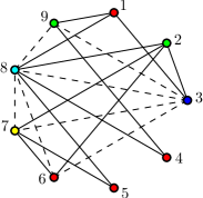
The colorful method partitions a matrix into sets of pairwise conflict-free rows. Here we distinguish between two kinds of conflicts. If a thread owns row and a second thread owning row , , requires to modify , , it is called an indirect conflict. If , we call such conflict direct. The conflict graph of a matrix is the graph , where each vertex corresponds to a row in , and the edges in represent conflicts between vertices. Figure LABEL:sub@fig:conflicts shows the conflict graph for the matrix in Figure 1. Direct and indirect conflicts are indicated by solid and dashed lines, respectively. In the graph, there are 12 direct and 7 indirect conflicts.
The direct conflicts of row are exactly the rows corresponding to the column indices of the non-zero entries at that row, i.e., the indices , . They can be computed in a single loop through the CSRC structure. The computation of indirect conflicts is more demanding. In our implementation, these are determined with the aid of the induced subgraph spanned by the edges in associated with direct conflicts. Given two vertices , if the intersection of their neighborhood in is non-empty, then they are indirectly in conflict.
We color the graph by applying a standard sequential coloring algorithm [8]. The color classes correspond to conflict-free blocks where the matrix-vector product can be safely carried out in parallel. Observe that coloring rectangular matrices is the same as coloring only its square part, since the rectangular part is accessed by rows. The layout of a 5-colored matrix is depicted in Figure LABEL:sub@fig:partitioning-colorful.
Let denote the number of colors used by the coloring algorithm. Suppose that the color classes are evenly sized, and that the loop over the rows is implemented as a divide-and-conquer recursion. Under such hypothesis, the span of the colorful method can be approximated by . Thus, the colorful matrix-vector product has a parallelism of . Although would lead to a better scalability when compared to the local buffers strategy, the possibility of exploiting systems based on cache hierarchies decreases, which affects considerably the code performance. Furthermore, the number of processors used in our experiments was always smaller than the number of colors.
4 Experimental results
Our implementation was evaluated on two Intel processors, including an Intel Core 2 Duo E8200 (codenamed Wolfdale) and an Intel i7 940 (codenamed Bloomfield). The Wolfdale processor runs at 2.66GHz, with L2 cache of 6MB and 8GB of RAM, and the Bloomfield one runs at 2.93GHz with 256KB L2 caches, 8MB of L3 cache and 8GB of RAM. Our interest on Intel Core 2 Duo machines lies on the fact that our finite element simulations are carried out on a dedicated 32-nodes cluster of such processors.
The code was parallelized using OpenMP directives, and compiled with Intel Fortran compiler (ifort) version 11.1 with level 3 optimizations (-O3 flag) enabled. Machine counters were accessed through the PAPI 3.7.1 library API [5]. The measurements of speedups and Mflop/s were carried out with PAPI instrumentation disabled.
The tests were performed on a data set comprised of 60 matrices, from which 32 are numerically symmetric. There is one non-symmetric dense matrix of order 1K, 50 matrices selected from the University of Florida sparse matrix collection [10], and 3 groups of 3 matrices each, called angical, tracer, and cube2m, of our own devise. Inside these groups, matrices correspond to one global finite element matrix output by our sequential finite element code, and two global matrices for both of the adopted domain partitioning schemes, overlapping (suffix “_o32”) and non-overlapping (suffix “_n32”), where 32 stands for the number of sub-domains. Our benchmark computes the sparse matrix-vector product a thousand times for each matrix in Table 1, which is a reasonable value for iterative solvers like the preconditioned conjugate gradient method and the generalized minimum residual method. All results correspond to median values over three of such runs.
| Matrix | Sym. | (KB) | |||
|---|---|---|---|---|---|
| thermal | no | 3456 | 66528 | 19 | 710 |
| ex37 | no | 3565 | 67591 | 18 | 722 |
| flowmeter5 | no | 9669 | 67391 | 6 | 828 |
| piston | no | 2025 | 100015 | 49 | 1012 |
| SiNa | yes | 5743 | 102265 | 17 | 1288 |
| benzene | yes | 8219 | 125444 | 15 | 1598 |
| cage10 | no | 11397 | 150645 | 13 | 1671 |
| spmsrtls | yes | 29995 | 129971 | 4 | 1991 |
| torsion1 | yes | 40000 | 118804 | 2 | 2017 |
| minsurfo | yes | 40806 | 122214 | 2 | 2069 |
| wang4 | no | 26068 | 177196 | 6 | 2188 |
| chem_master1 | no | 40401 | 201201 | 4 | 2675 |
| dixmaanl | yes | 60000 | 179999 | 2 | 3046 |
| chipcool1 | no | 20082 | 281150 | 14 | 3098 |
| t3dl | yes | 20360 | 265113 | 13 | 3424 |
| poisson3Da | no | 13514 | 352762 | 26 | 3682 |
| k3plates | no | 11107 | 378927 | 34 | 3895 |
| gridgena | yes | 48962 | 280523 | 5 | 4052 |
| cbuckle | yes | 13681 | 345098 | 25 | 4257 |
| bcircuit | no | 68902 | 375558 | 5 | 4878 |
| angical_n32 | yes | 20115 | 391473 | 19 | 4901 |
| angical_o32 | no | 18696 | 732186 | 39 | 4957 |
| tracer_n32 | yes | 33993 | 443612 | 13 | 5729 |
| tracer_o32 | no | 31484 | 828360 | 26 | 5889 |
| crystk02 | yes | 13965 | 491274 | 35 | 5975 |
| olafu | yes | 16146 | 515651 | 31 | 6295 |
| gyro | yes | 17361 | 519260 | 29 | 6356 |
| dawson5 | yes | 51537 | 531157 | 10 | 7029 |
| ASIC_100ks | no | 99190 | 578890 | 5 | 7396 |
| bcsstk35 | yes | 30237 | 740200 | 24 | 9146 |
| Matrix | Sym. | (KB) | |||
|---|---|---|---|---|---|
| dense_1000 | no | 1000 | 1000000 | 1000 | 9783 |
| sparsine | yes | 50000 | 799494 | 15 | 10150 |
| crystk03 | yes | 24696 | 887937 | 35 | 10791 |
| ex11 | no | 16614 | 1096948 | 66 | 11004 |
| 2cubes_sphere | yes | 101492 | 874378 | 8 | 11832 |
| xenon1 | no | 48600 | 1181120 | 24 | 12388 |
| raefsky3 | no | 21200 | 1488768 | 70 | 14911 |
| cube2m_o32 | no | 60044 | 1567463 | 26 | 16774 |
| nasasrb | yes | 54870 | 1366097 | 24 | 16866 |
| cube2m_n32 | no | 65350 | 1636210 | 25 | 17127 |
| venkat01 | no | 62424 | 1717792 | 27 | 17872 |
| filter3D | yes | 106437 | 1406808 | 13 | 18149 |
| appu | no | 14000 | 1853104 | 132 | 18342 |
| poisson3Db | no | 85623 | 2374949 | 27 | 24697 |
| thermomech_dK | no | 204316 | 2846228 | 13 | 31386 |
| Ga3As3H12 | yes | 61349 | 3016148 | 49 | 36304 |
| xenon2 | no | 157464 | 3866688 | 24 | 40528 |
| tmt_sym | yes | 726713 | 2903837 | 3 | 45384 |
| CO | yes | 221119 | 3943588 | 17 | 49668 |
| tmt_unsym | no | 917825 | 4584801 | 4 | 60907 |
| crankseg_1 | yes | 52804 | 5333507 | 101 | 63327 |
| SiO2 | yes | 155331 | 5719417 | 36 | 69451 |
| bmw3_2 | yes | 227362 | 5757996 | 25 | 71029 |
| af_0_k101 | yes | 503625 | 9027150 | 17 | 113656 |
| angical | yes | 546587 | 11218066 | 20 | 140002 |
| F1 | yes | 343791 | 13590452 | 39 | 164634 |
| tracer | yes | 1050374 | 14250293 | 13 | 183407 |
| audikw_1 | yes | 943695 | 39297771 | 41 | 475265 |
| cube2m | no | 2000000 | 52219136 | 26 | 545108 |
| cage15 | no | 5154859 | 99199551 | 19 | 1059358 |
4.1 Sequential performance
We have compared the sequential performance of CSRC to the standard CSR. For symmetric matrices, we have chosen the OSKI implementation [19] as the representative of the symmetric CSR algorithm, assuming that only the lower part of is stored.
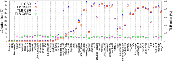
In the sparse matrix-vector product, each element of the matrix is accessed exactly once. Thus, accessing these entries incurs only on compulsory misses. On the other hand, the elements of and are accessed multiple times. This would enable us to take advantage of cache hierachies by reusing recently accessed values. In the CSR, the access pattern of the vector is known to be the major hindrance to the exploitation of data reuse, because arrays , , and all have stride-1 accesses. Since the vector is not traversed using unit stride anymore in the CSRC, one could argue that there would be an increase in the number of cache misses. As presented in Figure 4, experiments on L2 data cache misses suggest just the converse, while the ratio of TLB misses is roughly constant.
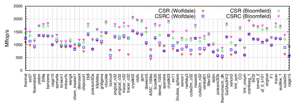
The performance of the algorithm considered herein is memory bounded, because the number of load/store operations is at least as greater as the number of floating-point multiply-add instructions. In a dense matrix-vector product, we need to carry out operations on amount of data, while for sparse matrices, these quantities are both . In particular, observe that the computation of the square product using the CSRC requires the execution of multiply and multiply-add operations, whereas the CSR algorithm requires multiply-add operations. On systems without fused multiply-add operations, the CSR and CSRC algorithms would perform and floating-point instructions, respectively. On the other hand, the number of load instructions for CSR is , and for the CSRC format. Hence the ratio between loadings and flops is approximately 1.26 for CSRC and exactly 1.5 for CSR. This bandwidth mitigation may be the most relevant reason for the efficiency of CSRC shown in Figure 5. It is also worth noting the advantage of the augmented CSRC on matrices whose square part is numerically symmetric, i.e., the matrices angical_o32 and tracer_o32.
4.2 Multi-thread version
Our parallel implementation was evaluated with up to 4 threads on Bloomfield with Hyper-Threading technology disabled. The values of speedup are relative to the pure sequential CSRC algorithm, and not to the one thread case.
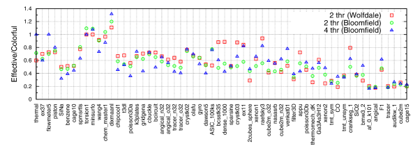
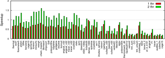
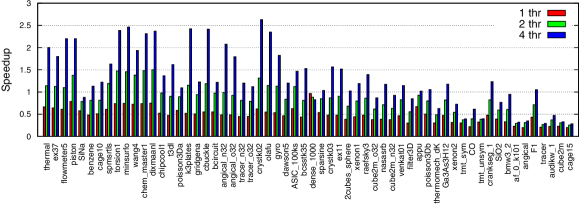
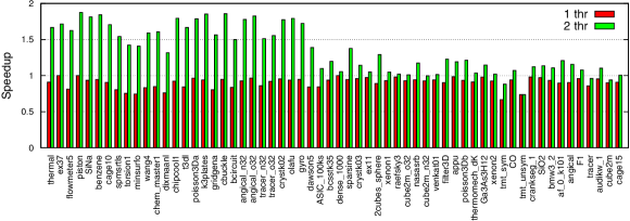
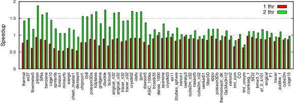
One would expect that the colorful method is best suited to matrices with few conflicts, e.g., narrow band matrices, because the lower is the maximum degree in the conflict graph, the larger is its parallelism. As shown in Figure 6, it was more efficient only on the matrices torsion1, minsurfo and dixmaanl, which have the smallest bandwidth among all matrices. Nonetheless, according to Figures LABEL:sub@fig:wolfdale-matvec_bench-colorful-speedup and LABEL:sub@fig:bloomfield-matvec_bench-colorful-speedup, small matrices can still benefit from some parallelism.
An important deficiency of the colorful strategy, which contributes to its lack of locality, is the variable-size stride access to the source and destination vectors. Inside each color, there not exist rows sharing neither nor positions, because if they do share there will be a conflict, therefore they must have different colors. We claim that there must be an optimal color size to compensate such irregular accesses.
| (a) |
 (a)
(a)
|
|---|---|
| (b) |
 (b)
(b)
|
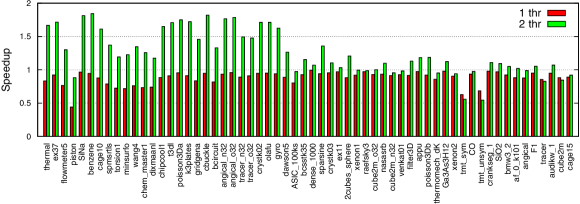
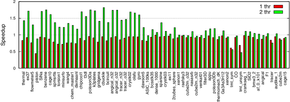
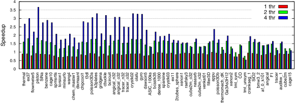
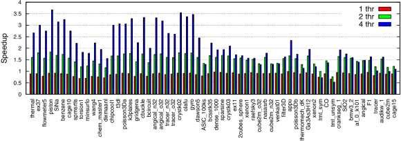
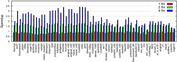
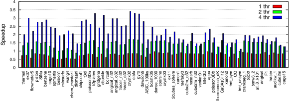
Figures 8 and 9 show the outcomes of speedups attained by all four implementations of the local buffers strategy. The overheads due to the initialization and accumulation steps become notorious when using just one thread. This can be easily overcome by checking the number of threads at runtime. If there exists only one thread in the working team, the global destination vector is used instead. Although all four implementations reached reasonable speedup peaks, the effective method has been more stable over the whole data set. On the average, it is the best choice for 93% of the cases on the Wolfdale, and for 80% and 78% on Bloomfield with 2 and 4 threads, respectively.
| (a) |
 (a)
(a)
|
|---|---|
| (b) |
 (b)
(b)
|
| (c) |
 (c)
(c)
|
| (d) |
 (d)
(d)
|
| (a) |
 (a)
(a)
|
|---|---|
| (b) |
 (b)
(b)
|
| (c) |
 (c)
(c)
|
| (d) |
 (d)
(d)
|
To better illustrate the performance of different initialization/accumulation algorithms, Table 2 presents average values of the running time consumed by these algorithms considering two classes of matrices, the ones that fit in cache and the others that do not. As expected, both all-in-one and per buffer strategies have similar performance. The effective and interval methods have demonstrated to be very feasible for practical use, although the later may incur a higher overheard because the number of intervals is at least as great as the number of threads.
In general, the running time is influenced by the working set size and the band structure of the matrix. When the arrays used by the CSRC fit or nearly fit into cache memory, better speedups were obtained with almost linear scalability, reaching up to 1.87 on Wolfdale. For some matrices from the University of Florida collection it was observed a poor performance, e.g., tmt_sym, tmt_unsym, cage15 and F1. In the case of cage15 and F1, this may be attributed to the absence of a band structure. On the other hand, there seems to be a bandwidth lower bound for preserving performance. In particular, the quasi-diagonal profile of the matrices tmt_sym and tmt_unsym have contributed to amplify indirection overheads.
Our code has been 63% more efficient on Bloomfield using 2 threads than on Wolfdale. Taking a closer view, however, we see that Wolfdale is faster on 80% of matrices with working set sizes up to 8MB, while Bloomfield beats the former on 94% of the remaining matrices. Notice that Wolfdale requires less cycles than Bloomfield to access its outer most cache, which would explain its superiority on small matrices.
Analysing the performance with 4 threads on the Bloomfield processor shown in Figure LABEL:sub@fig:bloomfield-matvec_bench-local_buffers_effective_nonzeros-speedup, speedups indicate that large working sets drastically degrades the efficiency of the implementation, compared to the 2-threaded case. On smaller matrices, speedups seem to grow linearly, with peaks of 1.83 and 3.40 using 2 and 4 threads, respectively.
| Method | Wolfdale | Bloomfield | ||||
|---|---|---|---|---|---|---|
| MB | MB | MB | MB | |||
| 2 | 2 | 2 | 4 | 2 | 4 | |
| all-in-one | 0.0455 | 4.3831 | 0.0370 | 0.0475 | 1.3127 | 2.5068 |
| per buffer | 0.0455 | 4.3876 | 0.0320 | 0.0393 | 1.8522 | 3.8299 |
| effective | 0.0215 | 1.8785 | 0.0176 | 0.0234 | 0.8094 | 1.2575 |
| interval | 0.0858 | 2.9122 | 0.0748 | 0.0456 | 1.3920 | 1.4939 |
5 Conclusion
We have been concerned with the parallelization of the matrix-vector multiplication algorithm using the CSRC data structure, focusing on multi-core architectures. It has been advocated that multi-core parallelization alone can compete with purely sequential optimization techniques. We could observe that, provided sufficient memory bandwidth, our implementation has demonstrated to be fairly scalable.
The main deficiency of the colorful method is due to variable size stride accesses, which can destroy any locality provided by matrix reordering techniques. We claim that it could be improved by fixing the maximum allowed stride size inside each color class. This will be the objective of our future investigations.
Computing the transpose matrix-vector multiplication is considered costly when using the standard CSR. An easy but still expensive solution would be to convert it into the CSC format before spawning threads. This operation is very straightforward using the CSRC, as we just need to swap the addresses of and , and we are done. Clearly, the computational costs remain the same.
Our results extend previous work on the computation of the sparse matrix-vector product for structurally symmetric matrices to multi-core architectures. The algorithms hereby presented are now part of a distributed-memory implementation of the finite element method [26]. Currently, we conduct experiments on the effect of coupling both coarse- and fine-grained parallelisms.
Acknowledgment
We would like to thank Prof. José A. F. Santiago and Cid S. G. Monteiro for granting access to the Intel i7 machines used in our experiments. We are also grateful to Aydın Buluç and the anonymous reviewers for the helpful comments.
References
- [1] R. C. Agarwal, F. G. Gustavson, and M. Zubair. A high performance algorithm using pre-processing for the sparse matrix-vector multiplication. In Proc. 1992 ACM/IEEE conference on Supercomputing, pages 32–41, 1992.
- [2] G. O. Ainsworth Jr., F. L. B. Ribeiro, and C. Magluta. Parallel implementation of the implicitly restarted Arnoldi/Lanczos method. In Proc. 21st IASTED International Conference on Parallel and Distributed Computing and Systems, 2009. Track 668-033.
- [3] M. Belgin, G. Back, and C. J. Ribbens. Pattern-based sparse matrix representation for memory-efficient SMVM kernels. In Proc. 23rd International Conference on Supercomputing, pages 100–109, 2009.
- [4] G. E. Blelloch, M. A. Heroux, and M. Zagha. Segmented operations for sparse matrix computation on vector multiprocessors. Technical Report CMU-CS-93-173, School of Computer Science, Carnegie Mellon University, Pittsburgh, PA, USA, 1993.
- [5] S. Browne, J. Dongarra, N. Garner, G. Ho, and P. Mucci. A portable programming interface for performance evaluation on modern processors. International Journal of High Performance Computing Applications, 14(3):189–204, 2000.
- [6] A. Buluç, J. T. Fineman, M. Frigo, J. R. Gilbert, and C. E. Leiserson. Parallel sparse matrix-vector and matrix-transpose-vector multiplication using compressed sparse blocks. In Proc. 21st Annual Symposium on Parallelism in Algorithms and Architectures, pages 233–244, 2009.
- [7] U. V. Çatalyürek and C. Aykanat. Decomposing irregularly sparse matrices for parallel matrix-vector multiplication. In Proc. 3rd International Workshop on Parallel Algorithms for Irregularly Structured Problems, pages 75–86, 1996.
- [8] T. F. Coleman and J. J. Moré. Estimation of sparse jacobian matrices and graph coloring problems. SIAM Journal on Numerical Analysis, 20(1):187–209, 1983.
- [9] T. H. Cormen, C. E. Leiserson, R. L. Rivest, and C. Stein. Introduction to Algorithms. The MIT Press, Cambridge, MA, USA, 3rd edition, 2009.
- [10] T. A. Davis. The University of Florida sparse matrix collection, 1997.
- [11] E. F. D’Azevedo, M. R. Fahey, and R. T. Mills. Vectorized sparse matrix multiply for compressed row storage format. In Proc. 5th International Conference on Computational Science, pages 99–106, 2005.
- [12] R. Geus and S. Röllin. Towards a fast parallel sparse symmetric matrix-vector multiplication. Parallel Computing, 27(7):883–896, 2001.
- [13] G. Goumas, K. Kourtis, N. Anastopoulos, V. Karakasis, and N. Koziris. Performance evaluation of the sparse matrix-vector multiplication on modern architectures. Journal of Supercomputing, 50(1):36–77, 2009.
- [14] W. D. Gropp, D. K. Kaushik, D. E. Keyes, and B. F. Smith. Towards realistic performance bounds for implicit CFD codes. In Proc. 11th International Conference on Parallel Computational Fluid Dynamics, pages 233–240, 1999.
- [15] E.-J. Im, K. Yelick, and R. Vuduc. Sparsity: Optimization framework for sparse matrix kernels. International Journal of High Performance Computing Applications, 18(1):135–158, 2004.
- [16] E.-J. Im and K. A. Yelick. Optimizing sparse matrix vector multiplication on SMPs. In Proc. 9th SIAM Conference on Parallel Processing for Scientific Computing, 1999.
- [17] H. Kotakemori, H. Hasegawa, T. Kajiyama, A. Nukada, R. Suda, and A. Nishida. Performance evaluation of parallel sparse matrix-vector products on SGI Altix3700. In Proc. 1st International Workshop on OpenMP, pages 153–163, 2005.
- [18] K. Kourtis, G. Goumas, and N. Koziris. Improving the performance of multithreaded sparse matrix-vector multiplication using index and value compression. In Proc. 37th International Conference on Parallel Processing, pages 511–519, 2008.
- [19] B. C. Lee, R. W. Vuduc, J. W. Demmel, and K. A. Yelick. Performance models for evaluation and automatic tuning of symmetric sparse matrix-vector multiply. In Proc. 33rd International Conference on Parallel Processing, pages 169–176, 2004.
- [20] S. Liu, Y. Zhang, X. Sun, and R. Qiu. Performance evaluation of multithreaded sparse matrix-vector multiplication using OpenMP. In Proc. 10th IEEE International Conference on High Performance Computing and Communications, pages 659–665, 2009.
- [21] J. Mellor-Crummey and J. Garvin. Optimizing sparse matrix-vector product computations using unroll and jam. International Journal of High Performance Computing Applications, 18(2):225–236, 2004.
- [22] D. Moloney, D. Geraghty, C. McSweeney, and C. McElroy. Streaming sparse matrix compression/decompression. In Proc. 1st International Conference on High Performance Embedded Architectures & Compilers, pages 116–129, 2005.
- [23] R. Nishtala, R. W. Vuduc, J. W. Demmel, and K. A. Yelick. When cache blocking of sparse matrix vector multiply works and why. Applicable Algebra in Engineering, Communication and Computing, 18(3):297–311, 2007.
- [24] A. Pinar and M. T. Heath. Improving performance of sparse matrix-vector multiplication. In Proc. 1999 ACM/IEEE conference on Supercomputing, page 30, 1999.
- [25] F. L. B. Ribeiro and A. L. G. d. A. Coutinho. Comparison between element, edge and compressed storage schemes for iterative solutions in finite element analyses. International Journal for Numerical Methods in Engineering, 63(4):569–588, 2005.
- [26] F. L. B. Ribeiro and I. A. Ferreira. Parallel implementation of the finite element method using compressed data structures. Computational Mechanics, 41(18):31–48, 2007.
- [27] Y. Saad. Iterative methods for sparse linear systems. The PWS Series in Computer Science. PWS Publising Company, Boston, MA, USA, 1995.
- [28] O. Temam and W. Jalby. Characterizing the behavior of sparse algorithms on caches. In Proc. 1992 ACM/IEEE conference on Supercomputing, pages 578–587, 1992.
- [29] S. Toledo. Improving the memory-system performance of sparse-matrix vector multiplication. IBM Journal of Research and Development, 41(6):711–726, 1997.
- [30] R. Vuduc, J. W. Demmel, and K. A. Yelick. OSKI: A library of automatically tuned sparse matrix kernels. Journal of Physics: Conference Series, 16:521–530, 2005.
- [31] R. W. Vuduc and H.-J. Moon. Fast sparse matrix-vector multiplication by exploiting variable block structure. In Proc. 1st International Conference High Performance Computing and Communications, 2005.
- [32] J. B. White, III and P. Sadayappan. On improving the performance of sparse matrix-vector multiplication. In Proc. 4th International Conference on High-Performance Computing, pages 66–72, 1997.
- [33] J. Willcock and A. Lumsdaine. Accelerating sparse matrix computations via data compression. In Proc. 20th annual international conference on Supercomputing, pages 307–316, 2006.
- [34] S. Williams, L. Oliker, R. Vuduc, J. Shalf, K. Yelick, and J. Demmel. Optimization of sparse matrix-vector multiplication on emerging multicore platforms. Parallel Computing, 35(3):178–194, 2009.