Data analysis of gravitational-wave signals from spinning neutron stars.
V. A narrow-band all-sky search

Abstract

We present theory and algorithms to perform an all-sky coherent search for periodic signals of gravitational waves in narrow-band data of a detector. Our search is based on a statistic, commonly called the ${\mathcal{F}}$-statistic, derived from the maximum-likelihood principle in Paper I of this series. We briefly review the response of a ground-based detector to the gravitational-wave signal from a rotating neuron star and the derivation of the ${\mathcal{F}}$-statistic. We present several algorithms to calculate efficiently this statistic. In particular our algorithms are such that one can take advantage of the speed of fast Fourier transform (FFT) in calculation of the ${\mathcal{F}}$-statistic. We construct a grid in the parameter space such that the nodes of the grid coincide with the Fourier frequencies. We present interpolation methods that approximately convert the two integrals in the ${\mathcal{F}}$-statistic into Fourier transforms so that the FFT algorithm can be applied in their evaluation. We have implemented our methods and algorithms into computer codes and we present results of the Monte Carlo simulations performed to test these codes.

I Introduction

Periodic gravitational-wave signals like those originating from rotating neutron stars are an important class of sources that can be detected by currently operating ground-based detectors. Several methods were developed to search for such sources and several searches were performed. This paper continues the series of papers JKS98 ; JK99 ; JK00 ; ABJK02 devoted to studies of data analysis tools and algorithms needed to perform an all-sky coherent search for quasiperiodic gravitational waves.

The search presented in the current paper is based on the maximum-likelihood statistic called the ${\mathcal{F}}$-statistic that we have derived in the Paper I JKS98 of this series. It is known that the coherent search for long observation time needed to detect weak gravitational-wave signals from rotating neutron stars are computationally prohibitive (see BCCS98 and Paper III of this series JK00 ). Promising strategies are hierarchical semi-coherent methods. In these methods data is broken into short segments. In the first stage each segment is analyzed using the ${\mathcal{F}}$-statistic and in the second stage the ${\mathcal{F}}$-statistics from the short segments are combined using a certain algorithm. There are several methods proposed for the second stage: search for coincidences among candidates from short duration segments LIGO07Fstat ; LIGO09EHa , stack-slide method BC99 , power flux method LIGO08powerflux ; LIGO09powerflux , Hough transform method PAFS97 ; PS99 ; KSPSFP04 ; LIGO05Hough ; LIGO08powerflux . Recently an optimal method for the second stage has been found, the global correlation coordinate method P08 ; AP09 , which exploits global parameter space correlations in the coherent detection statistic. In our paper we shall present methods to optimize the first, coherent stage of a hierarchical method.

The techniques presented in this paper were used in the analysis of NAUTILUS bar detector data Astone2008 and are presently used in the analysis of the VIRGO data. Alternative techniques for the coherent stage based on the ${\mathcal{F}}$-statistic and their application to the real data can be found in Refs. Astone2005 ; LIGO07Fstat ; LIGO09EHa ; LIGO09EHb

The paper is organized as follows. In Sec. II we present the noise-free response of a ground-based detector to a gravitational-wave signal from a rotating neutron star. This response was derived and discussed in detail in Papers I JKS98 and IV ABJK02 of our series. In Sec. III we present data analysis tools to perform coherent search of the data for a gravitational-wave signal given in Sec. II. In Sec. III.1 we present the ${\mathcal{F}}$-statistic that was derived in Paper I. We limit ourselves to the case when the observation time is an integer multiple of one sidereal day. This simplifies some general formulas considerably. In Sec. III.2 we introduce a simplified approximate model for a periodic gravitational-wave signal. This approximate signal has the constant amplitude and its phase is parameterized in such a way that it is a linear function of the parameters. For such a signal the Fisher matrix is constant and consequently it is independent of the values of the signal’s parameters. In Sec. III.3 we briefly review calculation of the false alarm probability. Section IV is devoted to construction of the grid of templates in the parameter space. The grid solves a certain covering problem with a constraint. Our constraint is that the nodes of the grid coincide with the Fourier frequencies. This allows to use the fast Fourier transform (FFT) algorithm to compute the ${\mathcal{F}}$-statistic at grid nodes, what greatly accelerates the calculation. In Sec. V we describe our package Top2Bary that is used to calculate the position and the velocity of the detector located on the Earth with respect to the solar system barycenter. In Sec. V.1 we introduce various concepts and definitions used in the astrometry and in Sec. V.2 we describe the content of our package which is a set of fortran routines. In Sec. VI we present various approximations that we use in the calculation of the ${\mathcal{F}}$-statistic in order to speed up computations. In Sec. VI A we discuss resampling of the time series to the barycenter that we need to perform before we can apply the FFT. We develop two algorithms: one slow and very accurate and the other fast but less accurate. We compare the two algorithms using the signal from Sec. II. In Sec. VI B we describe interpolation of the FFT in the Fourier domain. This interpolation method allows to obtain efficiently an FFT that is twice as fine as the FFT of original data. In Sec. VI C we describe the Nelder-Mead algorithm that we use to find accurately the maximum of the ${\mathcal{F}}$-statistic. In Sec. VII we perform a number of Monte Carlo simulations of the computer code where we have implemented the methods and algorithms from Secs. III–VI. In our simulations we investigate how well we estimate the parameters of the signal in comparison to the Cramér-Rao bound.

II Response of a detector to a periodic gravitational wave

The dimensionless noise-free response $h$ of a gravitational-wave detector to a weak plane gravitational wave in the long wavelength approximation [i.e., when the size of the detector is much smaller than the reduced wavelength $\lambda/(2\pi)$ of the wave] can be written as the linear combination of the two independent wave polarizations $h_{+}$ and $h_{\times}$,

$$h(t)=F_{+}(t)h_{+}(t)+F_{\times}(t)h_{\times}(t),$$ (1)

where $F_{+}$ and $F_{\times}$ are the detector’s beam-pattern functions, which are of the form

$$F_{+}(t) =\sin\zeta\big{(}a(t)\cos 2\psi+b(t)\sin 2\psi\big{)},$$ (2a)

$$F_{\times}(t) =\sin\zeta\big{(}b(t)\cos 2\psi-a(t)\sin 2\psi\big{)}.$$ (2b)

The beam-patterns $F_{+}$ and $F_{\times}$ are linear combinations of $\sin 2\psi$ and $\cos 2\psi$, where $\psi$ is the polarization angle of the wave. For interferometric detectors the angle $\zeta$ is the angle between the interferometer arms (usually $\zeta=90^{\circ}$) whereas for the case of bars one has to put $\zeta=90^{\circ}$. The functions $a(t)$ and $b(t)$ are amplitude modulation functions, which depend on the location of the detector on the Earth and on the position of the gravitational-wave source in the sky (described in the celestial coordinate system by the right ascension $\alpha$ and the declination $\delta$ of the source). They are periodic functions of time with the period of one sidereal day. Analytic form of the functions $a(t)$ and $b(t)$ depends on the type of the detector; for the case of bar detectors they are explicitly given in Eqs. (A11) of Ref. ABJK02 , whereas for interferometric detectors they can be found in Eqs. (12) and (13) of Ref. JKS98 .

We are interested in periodic waves, for which the wave polarization functions are of the form

$$h_{+}(t) =h_{0+}\cos(\phi(t)+\phi_{0}),$$ (3a)

$$h_{\times}(t) =h_{0\times}\sin(\phi(t)+\phi_{0}),$$ (3b)

where $h_{0+}$ and $h_{0\times}$ are constant amplitudes of the two polarizations and $\phi(t)+\phi_{0}$ is the phase of the wave (with $\phi_{0}$ being the initial phase of the waveform). The amplitudes $h_{0+}$ and $h_{0\times}$ depend on the physical mechanism generating gravitational radiation. E.g., if a neutron star is a triaxial ellipsoid rotating around a principal axis with frequency $f$, then these amplitudes are

$$h_{0+} =\frac{1}{2}h_{0}(1+\cos^{2}\iota),$$ (4a)

$$h_{0\times} =h_{0}\cos\iota,$$ (4b)

where $\iota$ is the angle between the star’s angular momentum vector and the direction from the star to the Earth, and the amplitude $h_{0}$ is given by

$$h_{0}=\frac{16\pi^{2}G}{c^{4}}\frac{\epsilon If^{2}}{r}.$$ (5)

Here $I$ is the star’s moment of inertia with respect to the rotation axis, $r$ is the distance to the star, and $\epsilon$ is the star’s ellipticity defined by $\epsilon=|I_{1}-I_{2}|/I$, where $I_{1}$ and $I_{2}$ are moments of inertia with respect to the principal axes orthogonal to the rotation axis.

We further assume that the gravitational waveform given by Eqs. (1)–(3) is almost monochromatic around some angular frequency $\omega_{0}$, which we define as instantaneous angular frequency evaluated at the solar system barycenter (SSB) at $t=0$. The phase modulation function $\phi(t)$ for such waveform is approximately given by

$$\phi(t)=\sum_{k=0}^{s}\omega_{k}\frac{t^{k+1}}{(k+1)!}+\frac{{\bf n}_{0}\cdot{\bf r}_{\rm d}(t)}{c}\sum_{k=0}^{s}\omega_{k}\frac{t^{k}}{k!},$$ (6)

where $\omega_{k}$ ($k=1,2,\ldots,s$) is the $k$th time derivative of the instantaneous angular frequency at the SSB evaluated at $t=0$, $\mathbf{n}_{0}$ is the constant unit vector in the direction of the star in the SSB reference frame (it depends on the right ascension $\alpha$ and the declination $\delta$ of the source), and $\mathbf{r}_{\mathrm{d}}$ is the vector joining the SSB with the detector. Approximations that lead to Eq. (6) are discussed in detail in Sec. II B and Appendix A of Paper I.

Let us associate the following coordinate system with the SSB reference frame. The $x$ axis of the system is parallel to the $x$ axis of the celestial coordinate system, the $z$ axis is perpendicular to the ecliptic and has direction of the orbital angular momentum vector of the Earth. In this SSB coordinate system the vector $\mathbf{n}_{0}$ has the components

$$\mathbf{n}_{0}=\left(\begin{array}[]{ccc}1&0&0\\ 0&\cos\varepsilon&\sin\varepsilon\\ 0&-\sin\varepsilon&\cos\varepsilon\end{array}\right)\left(\begin{array}[]{c}\cos\alpha\cos\delta\\ \sin\alpha\cos\delta\\ \sin\delta\end{array}\right),$$ (7)

where $\varepsilon$ is the obliquity of the ecliptic. The position vector ${\bf r}_{\rm d}$ of the detector with respect to the SSB has the components

$${\bf r}_{\rm d}=\left(\begin{array}[]{c}R^{x}_{\mathrm{ES}}\\[4.30554pt] R^{y}_{\mathrm{ES}}\\[4.30554pt] 0\end{array}\right)+\left(\begin{array}[]{ccc}1&0&0\\ 0&\cos\varepsilon&\sin\varepsilon\\ 0&-\sin\varepsilon&\cos\varepsilon\end{array}\right)\left(\begin{array}[]{c}R^{x}_{\mathrm{E}}\\[4.30554pt] R^{y}_{\mathrm{E}}\\[4.30554pt] R^{z}_{\mathrm{E}}\end{array}\right),$$ (8)

where $(R^{x}_{\mathrm{ES}},R^{y}_{\mathrm{ES}},0)$ are the components of the vector joining the SSB with the center of the Earth in the SSB coordinate system, and $(R^{x}_{\mathrm{E}},R^{y}_{\mathrm{E}},R^{z}_{\mathrm{E}})$ are the components of the vector joining the center of the Earth and the detector’s location in the celestial coordinate system. Making use of Eqs. (7) and (8) one can obtain the explicit formula for the scalar product ${\bf n}_{0}\cdot{\bf r}_{\rm d}(t)$:

$${\bf n}_{0}\cdot{\bf r}_{\rm d}(t) =\cos\alpha\cos\delta\big{(}R^{x}_{\mathrm{ES}}(t)+R^{x}_{\mathrm{E}}(t)\big{)}$$

$$\quad+(\sin\alpha\cos\delta\cos\varepsilon+\sin\delta\sin\varepsilon)R^{y}_{\mathrm{ES}}(t)$$

$$\quad+\sin\alpha\cos\delta\,R^{y}_{\mathrm{E}}(t)+\sin\delta\,R^{z}_{\mathrm{E}}(t).$$ (9)

The phase $\phi$ of the waveform given by Eq. (6) depends on the angular frequency $\omega_{0}$, the $s$ spin-down parameters $\omega_{k}$ $(k=1,\ldots,s)$, and on the angles $\alpha$, $\delta$ (through the vector $\mathbf{n}_{0}$). We call the parameters $(\omega_{0},\omega_{1},\ldots,\omega_{s},\alpha,\delta)$ the intrinsic parameters and the remaining ones $(h_{0+},h_{0\times},\phi_{0},\psi$) the extrinsic (or amplitude) parameters. As we shall see in the following section we only need to search for signals over the intrinsic parameter space. The whole signal $h$ depends on $s+7$ unknown parameters: $(h_{0+},h_{0\times},\phi_{0},\psi,\alpha,\delta,\omega_{0},\omega_{1},\ldots,\omega_{s})$.

The response function $h$ depends on the position of the detector with respect to the SSB. This position can be determined with a great accuracy using JPL Planetary and Lunar Ephemerides DE405/LE405 as described in Sec. V. The dominant term in the phase $\phi(t)$ is $\omega_{0}\,t$; typical gravitational-wave frequency $f_{0}:=2\pi/\omega_{0}$ is contained in the range from a few Hz to a few kHz. The gravitational-wave signal from a rotating neutron star is a nearly periodic signal that is weakly amplitude and phase modulated due to the intrinsic variation of star’s rotation frequency and the motion of the detector with respect to the star. Moreover the amplitude of this signal is expected to be very small. Consequently detection of the signal requires observation time $T_{\mathrm{o}}$ that is very long with respect to the gravitational-wave period $P_{0}:=2\pi/\omega_{0}$.

Combining Eqs. (1)–(3) together one can decompose the response $h$ into linear combination of four time-dependent components:

$$h(t)=\sum^{4}_{i=1}A_{i}\,h_{i}(t),$$ (10)

where the functions $h_{i}$ ($i=1,\dots,4$) are of the form

$$\begin{array}[]{c}h_{1}(t)=a(t)\cos\phi(t),\hskip 8.53581pth_{2}(t)=b(t)\cos\phi(t),\\[8.61108pt] h_{3}(t)=a(t)\sin\phi(t),\hskip 8.53581pth_{4}(t)=b(t)\sin\phi(t),\end{array}$$ (13)

and the four constant amplitudes $A_{i}$ ($i=1,\dots,4$) are given by

$$A_{i}={\bar{A}}_{i}\sin\zeta,\quad i=1,\dots,4,$$ (14)

where

$${\bar{A}}_{1} =h_{0+}\cos 2\psi\cos\phi_{0}-h_{0\times}\sin 2\psi\sin\phi_{0},$$ (15a)

$${\bar{A}}_{2} =h_{0+}\sin 2\psi\cos\phi_{0}+h_{0\times}\cos 2\psi\sin\phi_{0},$$ (15b)

$${\bar{A}}_{3} =-h_{0+}\cos 2\psi\sin\phi_{0}-h_{0\times}\sin 2\psi\cos\phi_{0},$$ (15c)

$${\bar{A}}_{4} =-h_{0+}\sin 2\psi\sin\phi_{0}+h_{0\times}\cos 2\psi\cos\phi_{0}.$$ (15d)

One can invert Eqs. (15) to obtain formulas for the parameters $h_{0+}$, $h_{0\times}$, $\phi_{0}$, and $\psi$ as functions of the amplitudes ${\bar{A}}_{i}$. Let us introduce quantities

$$A :={\bar{A}}_{1}^{2}+{\bar{A}}_{2}^{2}+{\bar{A}}_{3}^{2}+{\bar{A}}_{4}^{2},$$ (16a)

$$D :={\bar{A}}_{1}{\bar{A}}_{4}-{\bar{A}}_{2}{\bar{A}}_{3}.$$ (16b)

Then the amplitudes $h_{0+}$ and $h_{0\times}$ can be uniquely determined from the relations (we assume here, without loss of generality, that $h_{0+}>0$)

$$h_{0+} =\sqrt{\frac{1}{2}\Big{(}A+\sqrt{A^{2}-4D^{2}}\Big{)}},$$ (17a)

$$h_{0\times} =\mbox{sign}(D)\sqrt{\frac{1}{2}\Big{(}A-\sqrt{A^{2}-4D^{2}}\Big{)}}.$$ (17b)

The initial phase $\phi_{0}$ and the polarization angle $\psi$ can be obtained from the following equations:

$$\tan 2\phi_{0} =\frac{2({\bar{A}}_{1}{\bar{A}}_{3}+{\bar{A}}_{2}{\bar{A}}_{4})}{{\bar{A}}_{3}^{2}+{\bar{A}}_{4}^{2}-{\bar{A}}_{1}^{2}-{\bar{A}}_{2}^{2}},$$ (18a)

$$\tan 4\psi =\frac{2({\bar{A}}_{1}{\bar{A}}_{2}+{\bar{A}}_{3}{\bar{A}}_{4})}{{\bar{A}}_{1}^{2}+{\bar{A}}_{3}^{2}-{\bar{A}}_{2}^{2}-{\bar{A}}_{4}^{2}}.$$ (18b)

Also Eqs. (4) can be solved for the amplitude $h_{0}$ and the angle $\iota$. The result is

$$h_{0} =h_{0+}+\sqrt{h_{0+}^{2}-h_{0\times}^{2}},$$ (19a)

$$\iota =\arccos(h_{0\times}/h_{0}).$$ (19b)

In the special case when the star’s angular momentum vector lies along the line of sight, $\cos\iota=\pm 1$, and the number of independent amplitude parameters is reduced to two. In this situation Eqs. (4) read (upper sign is for $\cos\iota=+1$ and lower sign is for $\cos\iota=-1$)

$$h_{0+}=h_{0},\quad h_{0\times}=\pm h_{0},$$ (20)

and Eqs. (15) simplify then to

$${\bar{A}}_{1} =h_{0}\cos(2\psi\pm\phi_{0}),$$ (21a)

$${\bar{A}}_{2} =h_{0}\sin(2\psi\pm\phi_{0}),$$ (21b)

$${\bar{A}}_{3} =\mp{\bar{A}}_{2},$$ (21c)

$${\bar{A}}_{4} =\pm{\bar{A}}_{1}.$$ (21d)

III Maximum-likelihood filtering

III.1 The ${\mathcal{F}}$-statistic

The gravitational-wave signal $h$ given by Eqs. (10) and (13) will be buried in the noise of a detector. We are thus faced with the problem of detecting the signal and estimating its parameters. A standard method is the method of maximum-likelihood (ML) detection that consists of maximizing the likelihood function, which we shall denote by $\Lambda$, with respect to the parameters of the signal. If the maximum of $\Lambda$ exceeds a certain threshold calculated from the false alarm probability that we can afford, we say that the signal is detected. The values of the parameters that maximize $\Lambda$ are said to be the maximum-likelihood estimators of the parameters of the signal. The magnitude of the maximum of $\Lambda$ determines the probability of detection of the signal.

We assume that the noise $n$ in the detector is an additive, stationary, Gaussian, and zero-mean continuous random process. Then the data $x$ (if the signal $h$ is present) can be written as

$$x(t)=n(t)+h(t).$$ (22)

The logarithm of the likelihood function has the form

$$\ln\Lambda=(x|h)-\frac{1}{2}(h|h),$$ (23)

where the scalar product $(\,\cdot\,|\,\cdot\,)$ is defined by

$$(x|y):=\frac{2}{\pi}\,\Re\int^{\infty}_{0}\frac{\tilde{x}(\omega)\tilde{y}^{*}(\omega)}{S_{h}(\omega)}\mathrm{d}\omega.$$ (24)

In Eq. (24) tilde denotes the Fourier transform, asterisk means complex conjugation, $S_{h}$ is the one-sided spectral density of the detector’s noise, and $\Re$ denotes the real part of a complex expression.

We further assume that over the frequency bandwidth of the signal $h$ the spectral density $S_{h}$ is nearly constant and equal to $S_{0}=S_{h}(\omega_{0})$, where $\omega_{0}$ is the frequency of the signal measured at the SSB at $t=0$. Then the scalar products entering Eq. (23) can be approximated by

$$(x|h) \approx\frac{2}{S_{0}}\int^{T_{\mathrm{o}}}_{0}x(t)\,h(t)\,\mathrm{d}t,$$ (25a)

$$(h|h) \approx\frac{2}{S_{0}}\int^{T_{\mathrm{o}}}_{0}\big{(}h(t)\big{)}^{2}\,\mathrm{d}t,$$ (25b)

where $T_{\mathrm{o}}$ is the observation time, and the observation interval is $\left\langle 0,T_{\mathrm{o}}\right\rangle$. It is useful to introduce the following notation

$$\left\langle x\right\rangle:=\frac{1}{T_{\mathrm{o}}}\int_{0}^{{T_{\mathrm{o}}}}x(t)\,\mathrm{d}t.$$ (26)

After applying this notation and making use of Eqs. (25), the log likelihood ratio from Eq. (23) can be written as

$$\ln\Lambda\approx\frac{2{T_{\mathrm{o}}}}{S_{0}}\left(\left\langle xh\right\rangle-\frac{1}{2}\left\langle h^{2}\right\rangle\right).$$ (27)

In Sec. III of Paper III we have analyzed in detail the likelihood ratio for the general case of a signal consisting of several narrow-band components. Here we only summarize the results of Paper III and adapt them to the case of our signal (10). The signal $h$ depends linearly on four amplitudes $A_{i}$. The likelihood equations for the ML estimators $\widehat{A}_{i}$ of the amplitudes $A_{i}$ are given by

$$\frac{\partial\ln\Lambda}{\partial A_{i}}=0,\quad i=1,\ldots,4.$$ (28)

One can easily find the explicit analytic solution to Eqs. (28). To simplify formulas we assume that the observation time ${T_{\mathrm{o}}}$ is an integer multiple of one sidereal day, i.e., ${T_{\mathrm{o}}}=n(2\pi/\Omega_{\text{r}})$ for some positive integer $n$, where $\Omega_{\text{r}}$ is the rotational angular velocity of the Earth. Then the time average of the product of the functions $a$ and $b$ [see Eqs. (2)] vanishes, $\left\langle ab\right\rangle=0$, and the analytic formulas for the ML estimators of the amplitudes are given by

$$\begin{array}[]{c}\displaystyle\widehat{A}_{1}\approx 2\frac{\left\langle xh_{1}\right\rangle}{\left\langle a^{2}\right\rangle},\quad\displaystyle\widehat{A}_{2}\approx 2\frac{\left\langle xh_{2}\right\rangle}{\left\langle b^{2}\right\rangle},\\[12.91663pt] \displaystyle\widehat{A}_{3}\approx 2\frac{\left\langle xh_{3}\right\rangle}{\left\langle a^{2}\right\rangle},\quad\displaystyle\widehat{A}_{4}\approx 2\frac{\left\langle xh_{4}\right\rangle}{\left\langle b^{2}\right\rangle}.\end{array}$$ (29)

Explicit formulas for the time averages $\left\langle a^{2}\right\rangle$ and $\left\langle b^{2}\right\rangle$ can be found in Appendix B of Paper IV.

The reduced log likelihood function ${\mathcal{F}}$ or the ${\mathcal{F}}$-statistic is the log likelihood function (27) with the amplitude parameters $A_{i}$ replaced by their estimators $\widehat{A}_{i}$. By virtue of Eqs. (29) from Eq. (27) one gets

$${\mathcal{F}}\approx\frac{2}{S_{0}{T_{\mathrm{o}}}}\left(\frac{|F_{a}|^{2}}{\left\langle a^{2}\right\rangle}+\frac{|F_{b}|^{2}}{\left\langle b^{2}\right\rangle}\right),$$ (30)

where

$$F_{a} :=\int^{{T_{\mathrm{o}}}}_{0}x(t)\,a(t)\exp[-\mathrm{i}\phi(t)]\,\mathrm{d}t,$$ (31a)

$$F_{b} :=\int^{{T_{\mathrm{o}}}}_{0}x(t)\,b(t)\exp[-\mathrm{i}\phi(t)]\,\mathrm{d}t.$$ (31b)

The ML estimators of the signal’s parameters are obtained in two steps. Firstly, the estimators of the frequency, the spin-down parameters, and the angles $\alpha$ and $\delta$ are obtained by maximizing the functional ${\mathcal{F}}$ with respect to these parameters. Secondly, the estimators of the amplitudes $A_{i}$ are calculated from the analytic formulas (29) with the correlations $\left\langle xh_{i}\right\rangle$ evaluated for the values of the parameters obtained in the first step.

III.2 A linear model

In this subsection we introduce a useful approximate model of the gravitational-wave signal from a rotating neutron star. The model relies on (i) neglecting all spin downs in the phase modulation due to motion of the detector with respect to the SSB; and (ii) discarding this component of the vector ${\bf r}_{\rm d}$ (connecting the SSB and the detector) which is perpendicular to the ecliptic. These approximations lead to the following phase of the signal:

$$\phi_{\mathrm{lin}}(t)=\sum_{k=0}^{s}\omega_{k}\frac{t^{k+1}}{(k+1)!}+\alpha_{1}\mu_{1}(t)+\alpha_{2}\mu_{2}(t),$$ (32)

where $\alpha_{1}$ and $\alpha_{2}$ are new constant parameters,

$$\alpha_{1} :=\omega_{0}(\sin\alpha\cos\delta\cos\varepsilon+\sin\delta\sin\varepsilon),$$ (33a)

$$\alpha_{2} :=\omega_{0}\cos\alpha\cos\delta,$$ (33b)

and where $\mu_{1}(t)$ and $\mu_{2}(t)$ are known functions of time,

$$\mu_{1}(t) :=\frac{1}{c}\Big{(}R^{y}_{\mathrm{ES}}(t)+R^{y}_{\mathrm{E}}(t)\cos\varepsilon\Big{)},$$ (34a)

$$\mu_{2}(t) :=\frac{1}{c}\Big{(}R^{x}_{\mathrm{ES}}(t)+R^{x}_{\mathrm{E}}(t)\Big{)}.$$ (34b)

We also neglect the slowly varying modulation of the signal’s amplitude, so finally we approximate the whole signal $h(t)$ by

$$h(t)=A_{0}\cos\big{(}\phi_{\mathrm{lin}}(t)+\phi_{0}\big{)},$$ (35)

where $A_{0}$ and $\phi_{0}$ are the constant amplitude and initial phase, respectively. The above signal model is called linear because it has the property that its phase (32) is a linear function of the parameters.

It is convenient to represent the linear model of the gravitational-wave signal in the following form

$$h(t;\boldsymbol{\theta})=A_{0}\cos\bigg{(}\sum_{k=0}^{M}\xi_{k}m_{k}(t)+\phi_{0}\bigg{)},$$ (36)

where the vector $\boldsymbol{\theta}$ collects all the signal’s parameters, $\boldsymbol{\theta}:=(A_{0},\phi_{0},\boldsymbol{\xi})$, with the vector $\boldsymbol{\xi}$ comprising the parameters of the signal’s phase, $\boldsymbol{\xi}:=(\omega_{0},\omega_{1},\ldots,\omega_{s},\alpha_{1},\alpha_{2})$, so $\xi_{k}=\omega_{k}$ for $k=0,1,\ldots,s$, $\xi_{s+1}=\alpha_{1}$, $\xi_{s+2}=\alpha_{2}$; functions $m_{k}(t)$, $k=0,1,\ldots,s+2$, are known functions of time $t$: $m_{k}(t):=t^{k+1}/(k+1)!$ for $k=0,1,\ldots,s$, $m_{s+1}(t):=\mu_{1}(t)$, and $m_{s+2}(t):=\mu_{2}(t)$; finally, $M:=s+2$.

For the signal (36) we will compute the optimal signal-to-noise ratio $\rho$,

$$\rho:=\sqrt{(h|h)},$$ (37)

and the components of the Fisher information matrix $\Gamma$,

$$\Gamma_{k\ell}:=\Big{(}\frac{\partial h}{\partial\theta_{k}}\Big{|}\frac{\partial h}{\partial\theta_{\ell}}\Big{)}.$$ (38)

It is reasonable to assume that the observation time ${T_{\mathrm{o}}}$ is much longer than the period $P_{0}=2\pi/\omega_{0}$ of the gravitational wave (typically $P_{0}\lesssim 0.1$ s and ${T_{\mathrm{o}}}\gtrsim 1$ day). As a consequence

$$\left\langle\cos[n\phi_{\mathrm{lin}}(t)]\right\rangle\approx 0,\quad\left\langle\sin[n\phi_{\mathrm{lin}}(t)]\right\rangle\approx 0,$$ (39)

for any positive integer $n$. Making use of these approximations one easily computes from Eq. (37) the signal-to-noise ratio,

$$\rho\approx A_{0}\sqrt{\frac{{T_{\mathrm{o}}}}{S_{0}}},$$ (40)

and from Eq. (38) the components of the Fisher information matrix,

$$\Gamma_{A_{0}A_{0}}\approx\frac{\rho^{2}}{A_{0}^{2}},\quad\Gamma_{\phi_{0}\phi_{0}}\approx\rho^{2},$$ (41a)

$$\Gamma_{A_{0}\phi_{0}}\approx\Gamma_{A_{0}\xi_{k}}\approx 0,\quad k=0,\ldots,M,$$ (41b)

$$\Gamma_{\phi_{0}\xi_{k}}\approx\rho^{2}\left\langle m_{k}\right\rangle,\quad k=0,\ldots,M,$$ (41c)

$$\Gamma_{\xi_{k}\xi_{\ell}}\approx\rho^{2}\left\langle m_{k}m_{\ell}\right\rangle,\quad k,\ell=0,\ldots,M.$$ (41d)

Assuming that the signal (36) is buried in the stationary and Gaussian noise, one easily computes its ${\mathcal{F}}$-statistic,

$${\mathcal{F}}[x(t);\boldsymbol{\xi}]\approx\frac{2}{S_{0}{T_{\mathrm{o}}}}\left|\int^{{T_{\mathrm{o}}}}_{0}x(t)\exp\bigg{(}-\mathrm{i}\sum_{k=0}^{M}\xi_{k}m_{k}(t)\bigg{)}\mathrm{d}t\right|^{2},$$ (42)

where $x(t)$ are the data.

III.3 False alarm probability

Let us calculate the autocovariance function ${\cal C}$ of the ${\mathcal{F}}$-statistic (42) in the case when data is only noise. It is defined as

$${\cal C}(\boldsymbol{\xi},\boldsymbol{\xi}^{\prime}):=\rm{E}_{0}[{\mathcal{F}}(\boldsymbol{\xi}){\mathcal{F}}(\boldsymbol{\xi}^{\prime})]-\rm{E}_{0}[{\mathcal{F}}(\boldsymbol{\xi})]E_{0}[{\mathcal{F}}(\boldsymbol{\xi}^{\prime})],$$ (43)

where $\rm{E}_{0}$ is the expectation value when data is only noise. We find that $\mathrm{E}_{0}[{\mathcal{F}}(\boldsymbol{\xi})]=1$ and that

$${\cal C}(\boldsymbol{\tau})\approx\left\langle\cos\Big{(}\sum_{k}\tau_{k}m_{k}(t)\Big{)}\right\rangle^{2}+\left\langle\sin\Big{(}\sum_{k}\tau_{k}m_{k}(t)\Big{)}\right\rangle^{2},$$ (44)

where $\boldsymbol{\tau}:=\boldsymbol{\xi}-\boldsymbol{\xi}^{\prime}$. Thus the autocovariance function depends only on the difference of the parameters at two points but not on the parameters themselves.

The autocovariance ${\cal C}$ attains its maximum value equal 1 when $\boldsymbol{\tau}=\mathbf{0}$. Let us consider Taylor expansion of ${\cal C}$ around the maximum up to terms quadratic in $\boldsymbol{\tau}$,

$${\cal C}(\boldsymbol{\tau})\approx 1+\sum_{k}\frac{\partial{\cal C}(\boldsymbol{\tau})}{\partial\tau_{k}}\bigg{|}_{\boldsymbol{\tau}=\mathbf{0}}\tau_{k}+\frac{1}{2}\sum_{k,\ell}\frac{\partial^{2}{\cal C}(\boldsymbol{\tau})}{\partial\tau_{k}\partial\tau_{l}}\bigg{|}_{\boldsymbol{\tau}=\mathbf{0}}\tau_{k}\tau_{\ell}.$$ (45)

As ${\cal C}$ attains its maximum for $\boldsymbol{\tau}=\mathbf{0}$, we have

$$\frac{\partial{\cal C}(\boldsymbol{\tau})}{\partial\tau_{k}}\bigg{|}_{\boldsymbol{\tau}=\mathbf{0}}=0.$$ (46)

Let us introduce the symmetric matrix $G$ with elements

$$G_{k\ell}:=-\frac{1}{2}\frac{\partial^{2}{\cal C}(\boldsymbol{\tau})}{\partial\tau_{k}\partial\tau_{\ell}}\bigg{|}_{\boldsymbol{\tau}=\mathbf{0}}.$$ (47)

One can show that $G=\tilde{\Gamma}$, where $\tilde{\Gamma}$ is the reduced Fisher matrix defined by

$$\tilde{\Gamma}_{k\ell}:=\left\langle m_{k}m_{\ell}\right\rangle-\left\langle m_{k}\right\rangle\left\langle m_{\ell}\right\rangle.$$ (48)

For the linear phase model the components of the reduced Fisher matrix are constants independent of the values of the parameters. Making use of Eqs. (46)–(48), the Taylor expansion (45) can be written in the form

$${\cal C}(\boldsymbol{\tau})\approx 1-\sum_{k,\ell}\tilde{\Gamma}_{k\ell}\,\tau_{k}\,\tau_{\ell}.$$ (49)

We define now the correlation hypersurface of the statistic ${\mathcal{F}}$ by the requirement that the autocovariance $\mathcal{C}$ attains some constant value $\mathcal{C}_{0}$ on it:

$$\mathcal{C}(\boldsymbol{\tau})=\mathcal{C}_{0}.$$ (50)

This equality, by virtue of Eq. (49), can be written as

$$\sum_{k,\ell}\tilde{\Gamma}_{k\ell}\,\tau_{k}\,\tau_{\ell}=1-\mathcal{C}_{0}.$$ (51)

Equation (51) defines an $M$-dimensional hyperellipsoid.

The main idea is to divide the space of the phase parameters $\boldsymbol{\xi}$ into elementary cells which boundary is determined by Eq. (51). We choose the value $\mathcal{C}_{0}=1/2$. We estimate the number $N_{\mathrm{c}}$ of elementary cells by dividing the total Euclidean volume $V_{\text{total}}$ of the parameter space by the Euclidean volume $V_{\text{cell}}$ of the correlation hyperellipsoid, i.e., we have

$$N_{\mathrm{c}}=\frac{V_{\text{total}}}{V_{\text{cell}}},$$ (52)

where the Euclidean volume of one elementary cell equals

$$V_{\text{cell}}=\frac{\pi^{M/2}}{\Gamma(M/2+1)\sqrt{\det G}},$$ (53)

here $\Gamma$ denotes the Gamma function.

The values of the statistic ${\mathcal{F}}$ in different cells can be considered as independent random variables. We approximate the probability distribution of ${\mathcal{F}}$ in each cell by the probability distribution $p_{0}({\mathcal{F}})$ of ${\mathcal{F}}$ when the signal is absent. When the signal is absent, $2{\mathcal{F}}$ has a $\chi^{2}$ distribution with four degrees of freedom. The false alarm probability $P_{F}$ for a given cell is the probability that ${\mathcal{F}}$ exceeds a certain threshold ${\mathcal{F}}_{0}$ when there is no signal; for $\chi^{2}$ distribution with four degrees of freedom we have

$$P_{F}({\mathcal{F}}_{0})=(1+{\mathcal{F}}_{0})\exp(-{\mathcal{F}}_{0}).$$ (54)

The probability that ${\mathcal{F}}$ does not exceed the threshold ${\mathcal{F}}_{0}$ in a given cell is $1-P_{F}({\mathcal{F}}_{0})$, where $P_{F}({\mathcal{F}}_{0})$ is given by Eq. (54). Consequently the probability that ${\mathcal{F}}$ does not exceed the threshold ${\mathcal{F}}_{0}$ in all the $N_{\mathrm{c}}$ cells is $\big{(}1-P_{F}({\mathcal{F}}_{0})\big{)}^{N_{\mathrm{c}}}$. The probability $\alpha$ that ${\mathcal{F}}$ exceeds ${\mathcal{F}}_{0}$ in one or more cell is thus given by

$$\alpha=1-\big{(}1-P_{F}({\mathcal{F}}_{0})\big{)}^{N_{\mathrm{c}}}.$$ (55)

This is the desired false alarm probability. Inverting the formula (55) we can calculate the threshold value ${\mathcal{F}}_{0}$ corresponding to a chosen false alarm probability $\alpha$. The expected number of false alarms $N_{F}$ is given by

$$N_{F}=N_{\mathrm{c}}\,P_{F}({\mathcal{F}}_{0}).$$ (56)

IV Grid in the parameter space

In order to search for a signal in the noise of the detector we need to construct a grid in the space of the signal’s parameters. We define a grid in such a way that for any possible signal there exists a grid point in the parameter space such that the expectation value of the ${\mathcal{F}}$-statistic for the parameters of this grid point is greater than a certain value.

In the construction of the grid we employ the approximate linear model of the signal introduced in Sec.  III.2. The ${\mathcal{F}}$-statistic for this signal is given in Eq. (42). The expectation value of the ${\mathcal{F}}$-statistic, when the signal is present in the data [i.e., when the data $x(t)=n(t)+h(t;\boldsymbol{\theta})$, where $\boldsymbol{\theta}=(A_{0},\phi_{0},\boldsymbol{\xi})$ collects the signal’s parameters], is equal

$$\mathrm{E}_{1}\big{[}{\mathcal{F}}[n(t)+h(t;\boldsymbol{\theta});\boldsymbol{\xi}^{\prime}]\big{]}=1+\frac{\rho^{2}}{2}\mathcal{C}(\boldsymbol{\tau}),$$ (57)

where $\rho$ is the optimal signal-to-noise ratio computed in Eq. (40) and $\mathcal{C}$ is the autocovariance function given in Eq. (44); the vector $\boldsymbol{\tau}:=\boldsymbol{\xi}-\boldsymbol{\xi}^{\prime}$, where $\boldsymbol{\xi}^{\prime}$ are the phase parameters of the template. The function $\mathcal{C}$ has the maximum equal to 1 for $\boldsymbol{\tau}=\mathbf{0}$. The autocovariance function $\mathcal{C}$ is equal to the square of the match function $\mathcal{M}$ originally defined by Owen Owen96 .

To construct the grid we first choose the minimum value of the correlation that we can accept. We denote this value by $\mathcal{C}_{0}$. (Let us note that $\mathcal{C}_{0}=\text{MM}^{2}$, where MM is the minimal match introduced by Owen Owen96 .) Then we introduce, as in Sec.  III.3, the correlation hypersurface of the statistic ${\mathcal{F}}$ by the equality $\mathcal{C}(\boldsymbol{\tau})=\mathcal{C}_{0}$, which, after making the Taylor expansion of $\mathcal{C}$ up to the second order terms in $\boldsymbol{\tau}$, is described by Eq. (51).

IV.1 The covering problem with constraints

The problem of constructing a grid in the parameter space is equivalent to the so called covering problem Con ; prix07 : we want to cover $(M+1)$-dimensional parameter space with identical hyperellipsoids (51) in such a way that any point of the space belongs to at least one ellipsoid. Moreover, we look for an optimal covering, i.e., the one having smallest possible number of grid points per unit volume. The covering thickness $\theta$ is defined as the average number of ellipsoids that contain a point in the space. The optimal covering would have minimal possible thickness.

Let us introduce in the parameter space the new set of coordinates $\mathbf{x}=(x_{0},\ldots,x_{M})$, defined by the equality

$$\boldsymbol{\tau}={\mathsf{M}}\mathbf{x},$$ (58)

where the transformation matrix ${\mathsf{M}}$ is given by

$${\mathsf{M}}={\mathsf{U}}_{0}\,{\mathsf{D}}_{0}^{-1}.$$ (59)

Here ${\mathsf{D}}_{0}$ is the diagonal matrix whose diagonal components are square roots of eigenvalues of $\tilde{\Gamma}$, and ${\mathsf{U}}_{0}$ is a matrix whose columns are eigenvectors of $\tilde{\Gamma}$, normalized to unity. One can show that ${\mathsf{U}}_{0}$ is an orthogonal matrix, ${\mathsf{U}}_{0}^{-1}={\mathsf{U}}_{0}^{\mathrm{T}}$ (superscript ‘T’ denotes matrix transposition) and

$$\tilde{\Gamma}={\mathsf{U}}_{0}\,{\mathsf{D}}_{0}^{2}\,{\mathsf{U}}_{0}^{\text{T}}.$$ (60)

Hyperellipsoid (51) in coordinates $\mathbf{x}$ reduces to the $(M+1)$-dimensional sphere of radius $R:=\sqrt{1-\mathcal{C}_{0}}$. Therefore, the optimal grid can be expressed by means of a sphere covering.

In general, the thinnest possible coverings are known only in dimensions 1 and 2. In dimensions up to 5 the thinnest lattice coverings are known [see Eq. (63) below for the definition of a lattice], while in many higher dimensions the thinnest known coverings are lattices Con . From this point on we consider only lattice coverings. However, these general results cannot be easily adopted to our case. For computational reasons, we would like the nodes of the grid to coincide with Fourier frequencies, so that we can use the FFT algorithm to calculate the ${\mathcal{F}}$-satistic efficiently.

Our grid should meet the following constraint: one of its basis vectors needs to lie on the frequency axis and have given length. In other words, we look for the optimal covering with one of the lattice vectors fixed. We denote this vector by

$$\mathbf{a}_{0}=(\Delta{}p_{0},0,\ldots,0),$$ (61)

where $\Delta{}p_{0}$ is the fixed frequency resolution of our procedure. There is another constraint to be met in an all-sky search:

$$\mathbf{a}_{i}=(a_{i0},a_{i1},\ldots{},a_{is},0,0),\quad i=1,\ldots,s.$$ (62)

Having this constraint satisfied, we greatly reduce the computational overhead of resampling the data to the barycentric time (see Sec. VI.1).

As far as we know, the general solution to the covering problem with constraints is not known. Starting from the hypercubic covering (i.e., having all the lattice vectors orthogonal), a covering satisfying both constraints can be constructed, for the signal (36) with any number of parameters (see JKbook ). However, in higher dimensions it may be several times thicker than the thinnest unconstrained lattice known. An improved construction is proposed here, which takes as a starting point the thinnest lattice covering known in a given dimension, and applies a sequence of modifications to satisfy the constraints. We will refer to this lattice as the optimal covering.

IV.2 Optimal lattice

A lattice can be conveniently defined as a set of all linear combinations of its basis vectors $\mathbf{a}_{i}$ with integer coefficients:

$$\Lambda=\left\{\sum_{i}k_{i}\mathbf{a}_{i}:k_{i}\in\mathbb{Z}\right\}.$$ (63)

Given lattice $\Lambda$, its fundamental parallelotope is the set of all points of the form $\sum_{i}\theta_{i}\mathbf{a}_{i}$, with $0\leq\theta_{i}<1$. Fundamental parallelotope is one example of elementary cell. The thickness $\theta$ of a lattice covering is equal to the ratio of the volume of one hyperellipsoid to the volume of fundamental parallelotope.

For any lattice point $\mathbf{P}_{i}\in\Lambda$, the Voronoi cell around $\mathbf{P}_{i}$ is defined as

$$V(\mathbf{P}_{i})=\left\{\boldsymbol{\tau}:C(\boldsymbol{\tau}-\mathbf{P}_{i})\geq{}C(\boldsymbol{\tau}-\mathbf{P}_{j})\ \mathrm{for\ all}\ j\neq{}i\right\},$$ (64)

where $C(\boldsymbol{\tau})$ is the Taylor expansion (49) of the autocovariance function. All Voronoi cells of any lattice $\Lambda$ are congruent, disjoint, and their union is the whole space. Voronoi cell is another example of elementary cell and is sometimes called Wigner-Seitz cell or Brillouin zone. The Voronoi cell of $\Lambda$ is inscribed into the correlation ellipsoid (51).

Let $\Lambda$ be any lattice with basis vectors $(\mathbf{a}_{0},\mathbf{a}_{1},\dots)$. The square of minimal match of $\Lambda$ is

$$\mathrm{MM}^{2}(\Lambda)=\inf_{\boldsymbol{\tau}\in{}V(\mathbf{P}_{i})}C(\boldsymbol{\tau}-\mathbf{P}_{i}),$$ (65)

where $\mathbf{P}_{i}$ can be any lattice point. Let $\boldsymbol{\zeta}\in V(\mathbf{P}_{i})$ be the value for which the minimum in (65) is found. The function $C(\boldsymbol{\tau}-\mathbf{P}_{i})$ has at the point $\boldsymbol{\zeta}$ its absolute minimum inside the Voronoi cell $V(\mathbf{P}_{i})$, and $\boldsymbol{\zeta}$ is a deep hole of $\Lambda$. Note that the deep hole must be one of the vertices of the Voronoi cell. It makes Voronoi cells especially useful for calculating minimal match of a given lattice.

We can now outline the construction of an optimal covering in the parameter space. Given the value of $C_{0}$, we look for the thinnest possible lattice covering $\Lambda$, satisfying

$$\text{MM}^{2}(\Lambda)=C_{0}.$$ (66)

As a starting point, we consider the thinnest lattice covering known. It is determined by the number of phase parameters. For example, the thinnest covering of 4-dimensional space is the so called Voronoi’s principal lattice of the first type $A_{4}^{*}$ Con , having the thickness $\theta_{\mathrm{min}}=1.7655$. The generator matrix (a matrix whose rows are the basis vectors) of this lattice reads

$${\mathsf{M}}_{0}=R\sqrt{\frac{5}{2}}\begin{pmatrix}\sqrt{2}&0&0&0\\ \frac{1}{\sqrt{2}}&\sqrt{\frac{2}{3}}+\frac{1}{\sqrt{6}}&0&0\\ \frac{1}{\sqrt{2}}&\frac{1}{\sqrt{6}}&\frac{1}{2\sqrt{3}}+\frac{\sqrt{3}}{2}&0\\ -\frac{1}{5\sqrt{2}}-\frac{2\sqrt{2}}{5}&\frac{1}{5\sqrt{6}}-\frac{\sqrt{6}}{5}&-\frac{1}{5\sqrt{3}}-\frac{\sqrt{3}}{10}&-\frac{1}{2\sqrt{5}}\end{pmatrix},$$ (67)

where $R$ is the covering radius.

Let $\mathbf{l}$ be any lattice vector of $A_{4}^{*}$, such that $|\mathbf{l}|\geq{}|{\mathsf{M}}^{-1}\mathbf{a}_{0}|$, where ${\mathsf{M}}$ and $\mathbf{a}_{0}$ are given by Eqs. (59) and (61), respectively. The vector $\mathbf{l}$ is a linear combination of rows of (67). In order to construct an optimal lattice, satisfying constraint (61), we perform two scaling operations on $A_{4}^{*}$: shrinking in the direction of $\mathbf{l}$ by the factor $\mu=|{\mathsf{M}}^{-1}\mathbf{a}_{0}|/|\mathbf{l}|\leq{}1$ and expanding in all directions perpendicular to $\mathbf{l}$ by the factor $\nu\geq{}1$. The generator matrix of the shrunk lattice is

$${\mathsf{M}}_{1}={\mathsf{M}}_{0}\,{\mathsf{O}}_{1}\,\mathrm{diag}(\mu,1,1,1)\,{\mathsf{O}}_{1}^{-1},$$ (68)

where ${\mathsf{O}}_{1}$ is an orthogonal transformation defined by the condition that ${\mathsf{O}}_{1}(1,0,0,0)=\mathbf{l}/|\mathbf{l}|$.

The expansion factor $\nu$ is defined by the condition that the covering radius $R$ remains unchanged on scaling. In general, its value can be determined numerically using the following iteration:

$${\mathsf{M}}_{i+1}={\mathsf{M}}_{i}\,{\mathsf{O}}_{1}\,\mathrm{diag}(1,\nu_{i},\nu_{i},\nu_{i})\,{\mathsf{O}}_{1}^{-1},\quad\text{for $i=1,2,\dots$},$$ (69)

where $\nu_{i}=R/(R_{i}\sin{\phi_{i}})$, $R_{i}$ is the covering radius of the lattice given by ${\mathsf{M}}_{i}$, and $\phi_{i}\leq\pi/2$ is the largest angle that a half-line starting at the origin and containing a deep hole of ${\mathsf{M}}_{i}$ can form with the direction of $\mathbf{l}$. The above procedure converges after several iterations, and the expansion factor is formally $\nu=\prod_{i=1}^{\infty}\nu_{i}$.

After scaling, the lattice thickens by a factor $1/(\mu\nu^{3})\geq{}1$, depending on the choice of $\mathbf{l}$. Note that $\mu\nu^{3}\to{}0$ as the length of $\mathbf{l}$ increases. By enumerating the lattice vectors of $A_{4}^{*}$ in order of increasing magnitude, one can find the optimal $\mathbf{l}$, such that $1/(\mu\nu^{3})$ is minimal.

The generator matrix of an optimal lattice, satisfying the constraint (61), is

$${\mathsf{M}}_{\mathrm{opt}}={\mathsf{M}}_{0}\,{\mathsf{O}}_{1}\,{\mathsf{S}}\,{\mathsf{O}}_{2}^{-1}\,{\mathsf{M}}^{\mathrm{T}},$$ (70)

where ${\mathsf{O}}_{2}$ is an orthogonal transformation satisfying ${\mathsf{O}}_{2}(1,0,0,0)=\mathbf{e}_{0}/|\mathbf{e}_{0}|$ with $\mathbf{e}_{0}={\mathsf{M}}^{-1}\mathbf{a}_{0}$, ${\mathsf{S}}$ is a diagonal matrix with elements $(\mu,\nu,\nu,\nu)$. The lattice vector $\mathbf{l}$ is chosen in such a way that $\det{\mathsf{S}}$ is maximal. The thickness of this lattice is

$$\theta=\frac{\theta_{\mathrm{min}}}{\det{\mathsf{S}}}.$$ (71)

For the case of the Virgo antenna, observational time $T_{0}=2$ days, frequency 750 Hz, effective bandwidth 1 Hz, and $C_{0}=3/4$, the resulting lattice is thicker than $A_{4}^{*}$ only by 20%, $\theta\simeq{}2.1$, reducing the number of templates to roughly 10 millions (the corresponding hypercubic lattice would have 25 millions of templates).

The constraint (62) can be satisfied without increasing the lattice thickness by a 4-dimensional rotation ${\mathsf{O}}_{3}$ such that ${\mathsf{O}}_{3}\mathbf{e}_{0}=\mathbf{e}_{0}$ and the vector ${\mathsf{M}}{\mathsf{O}}_{3}{\mathsf{O}}_{2}{\mathsf{O}}_{1}^{-1}\mathbf{f}$ is orthogonal to the $(\alpha_{1},\alpha_{2})$ plane, where $\mathbf{f}$ is a lattice vector of $A_{4}^{*}$, $\mathbf{f}\nparallel{}\mathbf{l}$. The generator matrix of a lattice satisfying both constraints is now

$${\mathsf{M}}_{\mathrm{opt}}={\mathsf{M}}_{0}\,{\mathsf{O}}_{1}\,{\mathsf{S}}\,{\mathsf{O}}_{2}^{-1}\,{\mathsf{O}}_{3}^{-1}\,{\mathsf{M}}^{\mathrm{T}}.$$ (72)

IV.3 Two-dimensional example

Let us explain the construction of an optimal lattice on a simple, two-dimensional example. We consider here the signal

$$h(t;A_{0},\phi_{0},\bar{\omega}_{0},\bar{\omega}_{1})=A_{0}\cos\bigg{(}\bar{\omega}_{0}\frac{t}{{T_{\mathrm{o}}}}+\bar{\omega}_{1}\Big{(}\frac{t}{{T_{\mathrm{o}}}}\Big{)}^{2}+\phi_{0}\bigg{)},$$ (73)

where ${T_{\mathrm{o}}}$ is the observation time and the observation interval is $\left\langle 0,{T_{\mathrm{o}}}\right\rangle$. The phase of the signal (73) depends on two dimensionless parameters $\bar{\omega}_{0}$, $\bar{\omega}_{1}$ (and on the initial phase parameter $\phi_{0}$). The reduced Fisher matrix for this signal reads

$$\tilde{\Gamma}=\begin{pmatrix}\frac{1}{12}&\frac{1}{12}\\[4.30554pt] \frac{1}{12}&\frac{4}{45}\end{pmatrix}.$$ (74)

The correlation hypersurface (51) is now an ellipse:

$$\frac{(\tau_{1}+\tau_{2})^{2}}{12}+\frac{\tau_{2}^{2}}{180}=1-\mathcal{C}_{0}.$$ (75)

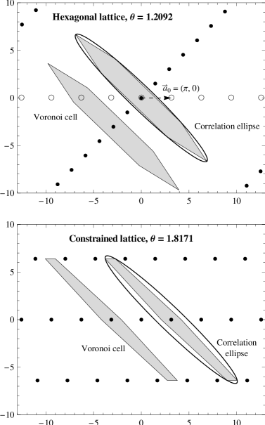
Correlation ellipse is shown on both parts of Fig. 1. Frequency resolution when calculating ${\mathcal{F}}$-statistic is now $\pi$, therefore we require the first basis vector of a lattice to be equal to

$$\mathbf{a}_{0}=(\pi,0),$$ (76)

in order to satisfy the constraint (61).

The thinnest possible covering in two dimensions is the hexagonal lattice, $A_{2}^{*}$. The Voronoi cell of $A_{2}^{*}$ is a regular hexagon, and the covering thickness is $\theta_{\text{hex}}=2\pi/(3\sqrt{3})\cong{}1.2092$. The generator matrix of $A_{2}^{*}$ is

$${\mathsf{M}}_{0}=R\sqrt{3}\begin{pmatrix}1&0\\ \frac{1}{2}&\frac{\sqrt{3}}{2}\end{pmatrix},$$ (77)

where $R=\sqrt{1-\mathcal{C}_{0}}$ is the covering radius. In order to cover the parameter space with ellipses (75), we have to transform the hexagonal lattice to the $\boldsymbol{\tau}\equiv(\tau_{1},\tau_{2})$ coordinates, as given by (58). The generator matrix of an optimal, hexagonal covering in $\boldsymbol{\tau}$ coordinates is

$${\mathsf{M}}_{\mathrm{hex}}={\mathsf{M}}_{0}\,{\mathsf{M}}^{\mathrm{T}}.$$ (78)

The resulting lattice is shown in the upper part of Fig. 1, along with the correlation ellipse. The Voronoi cell is a hexagon inscribed into the correlation ellipse (any lattice $\Lambda$ constitutes a covering if and only if the correlation hypersurface completely includes its Voronoi cell). Note that lattice points do not coincide with Fourier frequencies, represented by open circles.

The requirement (76) can be satisfied by the means of transformation (70), at the cost of increasing lattice thickness. We find that $|{\mathsf{M}}^{-1}\mathbf{a}_{0}|=\pi/(2\sqrt{3})$. For $\mathcal{C}_{0}=3/4$ (then $R=1/2$), the best choice of $\mathbf{l}$ is $\mathbf{l}=\sqrt{3}/4(3,\sqrt{3})$. The hexagonal lattice in coordinates $x_{i}$ is shrunk in the direction of $\mathbf{l}$ by the factor $\mu=|{\mathsf{M}}^{-1}\mathbf{a}_{0}|/|\mathbf{l}|=\pi/(3\sqrt{3})$, then expanded by the factor $\nu=\sqrt{108-\pi^{2}}/9$, and finally rotated in such a way that $\mathbf{l}$ coincides with ${\mathsf{M}}^{-1}\mathbf{a}_{0}$.

The lattice such obtained is shown in the lower part of Fig. 1. It has the thickness $\theta=\theta_{\mathrm{hex}}/(\mu\nu^{3})=18/\sqrt{108-\pi^{2}}\cong 1.8171$. Note that the Voronoi cell has changed. It covers more than half of the area of the correlation ellipse and is inscribed in it.

Figure 1: Up: Hexagonal covering generated by (78), with $\mathcal{C}_{0}=3/4$ and $R=1/2$ (dark points). Fourier frequencies are represented by open circles. Down: Constrained lattice, satisfying the condition (76). Any point in the parameter space belongs on average to 1.8171 ellipses.

V Position and velocity of a detector with respect to the solar system barycenter

In this section we describe algorithms and procedures needed to compute, for a given time and a geographical location of a detector, the corresponding vectors of position and velocity of the detector with respect to the Earth barycenter and of this barycenter with respect to the solar system barycenter (SSB). The sum of these vectors represents the position and velocity of the detector referred to the SSB.

We have incorporated the algorithms and procedures described in the present section into a set of fortran subroutines which we have called the Top2Bary package.

V.1 Overview of transformations involved

V.1.1 Reference systems and frames

Reference data for positional astronomy, such as the data in barycentric planetary ephemerides, are now specified within the International Celestial Reference System (ICRS). The ICRS is a coordinate system whose origin is at the SSB and whose axis directions are effectively defined by the adopted coordinates of 212 extragalactic radio sources which are assumed to have no observable intrinsic angular motions. Thus, the ICRS is a “space-fixed” system (more precisely, a kinematically non-rotating system) without an associated epoch. However, the ICRS closely matches the conventional dynamical system defined by the Earth’s mean equator and equinox of J2000.0; the alignment difference is at the 0.02 arcsecond level, negligible for many applications. The list of radio source positions that define ICRS for practical purposes is called the International Celestial Reference Frame (ICRF).

The position and velocity 3-vectors taken from the JPL DE405/LE405 ephemeris are in equatorial rectangular coordinates referred to the SSB. The reference frame for the DE405 is the ICRF; the alignment onto this frame, and therefore onto the ICRS, has an estimated accuracy of a few milliarcseconds, at least for the inner-planet data.

The DE405 was developed using T_eph, a barycentric coordinate time S98 . T_eph is rigorously equivalent to Barycentric Coordinate Time (TCB) in a mathematical sense, differing only in rate: the rate of T_eph matches the average rate of TT (Terrestrial Time, or TDT), while the rate of TCB is defined by the SI system. The IAU time scale, Barycentric Dynamical Time (TDB), often (but erroneously) considered to be the same as T_eph, is a quantity that cannot be physically realized, due to its flawed definition. So, in fact, the use of the name TDB actually refers to quantities based on or created with T_eph (because of this, the IAU Working Group on Nomenclature for Fundamental Astronomy has recommended changing the definition of TDB to be consistent with that of T_eph). Astronomical constants obtained from ephemerides based on T_eph (or TDB) are not in the SI system of units and must therefore be scaled for use with TCB or other SI-based time scales.

The epoch J2000.0 is the epoch of 2000 January 1, 12^h TT (JD 2451545.0 TT) at the geocenter (“J2000.0 system” is shorthand for the celestial reference system defined by the mean dynamical equator and equinox of J2000.0). The coordinate system defined by the “equator and equinox of J2000.0”, can be thought of as either barycentric or geocentric.

It is also worth noting that the recent IAU resolutions do not describe the proper reference system of the observer—the local, or topocentric, system in which most measurements are actually taken. The resolutions as adopted apply specifically to Einstein’s theory of gravity, i.e., the general theory of relativity.

V.1.2 Time scales

It is assumed that the time, associated with observational data we are dealing with, is the Coordinated Universal Time (UTC) as disseminated by international time services. The UTC scale since 1972 is essentially uniform, except for occasional 1 second steps (leap seconds) introduced internationally to compensate for the variable Earth rotation. By 2010 there were 24 leap seconds. Earlier, 1961 to 1971, the adjustments were continuous. UTC devoid of these adjustments is called the International Atomic Time, TAI. Addition of the difference TAI$-$UTC to UTC converts it to TAI which is uniform. TAI in turn differs from the Terrestrial (Dynamical) Time, TDT or TT (normally used to describe celestial phenomena by astronomers), only by a constant term:

$$\text{TDT}=\text{TAI}+32.184\,\mathrm{s}.$$

As already explained, the time argument of the JPL positions and velocities of celestial objects is in principle T_eph or the barycentric coordinate time. This time scale in practice can be equated with the Barycentric Dynamical Time, TDB (in spite of the noted inadequacy in its definition). The TDB differs from the TDT only by small periodic terms, which to sufficient accuracy are usually simplified to only two largest terms:

$$\text{TDB}-\text{TDT}=\big{(}0.001658\,\sin g+0.000014\,\sin 2g\big{)}\,\mathrm{s},$$

where $g=\big{(}357.53+0.9856003$ (JD$-$2451545.0)) degrees and JD is the Julian Date equal to MJD + 2400000.5, MJD being the Modified Julian Date. So essentially, the two scales do not have to be distinguished and for many practical purposes can be assumed equal, TDB$=$TDT.

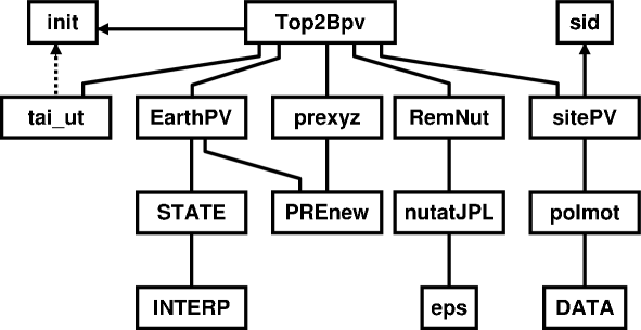
One can relate given UTC to barycentric positions of all the major celestial bodies of the solar system as obtainable from the JPL ephemeris. However, to relate the position of a point on the Earth to the geocentric ICRF (i.e., the same frame as the barycentric ICRF except for the origin of axes which is now at the barycenter of the Earth) one has to use yet another time scale—the rotational time scale UT1, which is nonuniform and is determined from astronomical observations. The difference UT1$-$UTC, the value of which is presently maintained by international services within $\pm 0.90$ s, is taken from the International Earth Rotation Service (IERS) tabulations of daily values publicly available as eopc04.yy files. The UT1 time can be readily converted to the Earth rotational angle or the sidereal time.

V.1.3 Location coordinates and velocities with respect to the Earth barycenter

To be able to express coordinates of a point on the Earth surface in the Earth centered ICRF, it is necessary to know orientation of the Earth in space. The primary effects that should be taken into account are: diurnal (variable) rotation, precession and nutation of the Earth rotational axis, and polar motion.

The precession is accounted for by applying standard astronomical theories. We use the new IAU theory Lieske1979 . The nutation also could be computed basing on a theory, but the DE405 has it in the numerical form, so we just read the nutation angles, $\Delta\psi$ and $\Delta\varepsilon$. These nutation angles are not the same as defined in the newest IAU nutation theory, so when highest precision is required the celestial pole offsets, d$\psi$ and d$\varepsilon$, must also be added to these angles (in the past the magnitude of these offsets remained below 0.1 arcsecond). For past years, since 1962, these two offsets are included in the already mentioned eopc04.yy files.

The remaining two effects, the Earth variable rotation and polar motion, are unpredictable for a remoter future, so also observational data must be used. The data necessary for reduction are taken from the eopc04.yy files as well. The polar motion can be taken into account by modifying the conventional geographical coordinates of a point on the Earth [see Eqs. (5.1) in ABJK02 ] or modifying the rectangular coordinates corresponding to these conventional geographical coordinates:

$$x_{\circ} =r_{\circ}\cos\lambda_{\circ},$$ (79a)

$$y_{\circ} =r_{\circ}\sin\lambda_{\circ},$$ (79b)

$$z_{\circ} =b\sin\Psi+h\sin\phi_{\circ},$$ (79c)

where $\phi_{\circ}$ is the conventional geographical latitude, $\lambda_{\circ}$ — the conventional longitude, $h$ — the height above the Earth ellipsoid, $\Psi=\arctan(b\tan\phi_{\circ}/a)$ — the reduced latitude, $r_{\circ}=a\cos\Psi+h\cos\phi_{\circ}$ is the equatorial component of the radius vector, and $a=6378.140$ km and $b=a(1-1/f)$ are the semiaxes of the ellipsoid (the flattening $f$ is taken equal to 1/0.00335281, which is the NOVAS value).

In this version we have adopted the second possibility (i.e. correcting of the Cartesian coordinates) using the following relations:

$$x =x_{\circ}-P_{x}z_{\circ},$$ (80a)

$$y =y_{\circ}+P_{y}z_{\circ},$$ (80b)

$$z =z_{\circ}+P_{x}x_{\circ}-P_{y}y_{\circ},$$ (80c)

where $P_{x}$ and $P_{y}$ are the IERS coordinates of the pole, with respect to the Conventional International Origin (to which the ‘conventional’ geographical coordinates refer), converted to radians.

These $(x,y,z)$ coordinates are expressed in the terrestrial reference frame with the $x$ axis directed toward the Greenwich meridian. To relate them to the celestial frame, the ICRF, the rotational angle of the Earth must be taken into account. This is done through conversion of UTC to UT1 (as described in the preceding subsection). The UT1 time serves to calculate the apparent (or true) local sidereal time $\theta$ (returned by the sid function), which includes the nutational component (nutation in longitude corrected for the corresponding IERS celestial pole offset also taken from the IERS eopc04 files). The apparent local time is advanced with respect to the mean Greenwich sidereal time by the true location longitude [calculated as $\lambda=\arctan(y/x)$ with proper choice of one of the four quadrants] and the mentioned nutational component. This component is equal to the so called equation of equinoxes $(\Delta\psi+\mathrm{d}\psi)\cos\varepsilon$ plus a very small correction to this equation (which amounts to less than $0.003^{\prime\prime}$ and depends on the mean longitude of the ascending node of the Moon).

So computed local sidereal time $\theta$ is finally used to find rectangular coordinates of the location in the geocentric ICRF:

$$X =r_{e}\cos\theta,$$ (81a)

$$Y =r_{e}\sin\theta,$$ (81b)

$$Z =z,$$ (81c)

where $r_{e}=\sqrt{x^{2}+y^{2}}$ is the equatorial component.

At this point the location velocity due to Earth rotation can be computed. The location motion relative to the Earth barycenter is represented by a vector of constant length [in principle, $v_{\circ}=2\pi r_{e}/(\text{sidereal day})=\Omega_{\text{r}}r_{e}$, where $\Omega_{\text{r}}$ is the Earth angular rotation speed] and directed always towards the east in the topocentric reference frame. This diurnal velocity vector has the following Cartesian components:

$$V_{x} =v_{\circ}\cos(\theta+\pi/2)=-v_{\circ}\sin\theta,$$ (82a)

$$V_{y} =v_{\circ}\sin(\theta+\pi/2)=+v_{\circ}\cos\theta,$$ (82b)

$$V_{z} =0,$$ (82c)

where the numerical value of $v_{\circ}$ is calculated with the NOVAS constant of the Earth angular rotation speed, $\Omega_{\text{r}}=2\pi/$(sidereal day in TAI seconds)$=7.2921151467\times 10^{-5}$ rad/s.

Since our approach is essentially classical, these Cartesian coordinates ($X,Y,Z$) and velocities ($V_{x},V_{y},V_{z}$) are naturally referred to the frame of equator and equinox of date. Therefore they are further nutated and precessed (in this order) back to the standard epoch J2000.0.

V.1.4 Barycentric coordinates of the Earth (JPL ephemeris)

For computing the coordinates of the Earth barycenter, relative to the SSB, use is made of the fundamental solar system ephemerides from the Jet Propulsion Laboratory (JPL). The latest JPL Planetary and Lunar Ephemerides, DE405/LE405 or just DE405, were created in 1997 and are described in detail in Ref. S98 . The DE405 ephemeris is based upon the ICRF. It constitutes of a set of Chebyshev polynomials fit with full precision to a numerical integration over 1600 AD to 2200 AD. The JPL package allows to obtain the rectangular coordinates of the Sun, Moon, and nine major planets anywhere between JED (i.e., Julian Ephemeris Date) 2305424.50 (1599 Dec 09) and JED 2525008.50 (2201 Feb 20). Besides coordinates, it includes nutations and librations.

The ephemeris gives separately the position and velocity of the Earth-Moon barycenter and the Moon’s position and velocity relative to this barycenter. The Earth position and velocity vectors (relative to the Earth-Moon barycenter) are thus calculated as a fraction (involving the masses of the two bodies) of the Moon’s vectors and opposite to them. For example, the $x$ coordinate of the Earth barycenter with respect to the SSB is obtained as:

$$x_{\text{E}}=x_{\text{EM}}-x_{\text{M}}/82.30056,$$

where ‘EM’ and ‘M’ subscripts refer to the Earth-Moon barycenter and the Moon, respectively, and the numerical denominator is equal to the Earth-plus-Moon to Moon ratio of masses taken from the JPL ephemeris. Similar expressions pertain to the $y_{\text{E}}$ and $z_{\text{E}}$ coordinates. Since the DE405/LE405 coordinates are given in the J2000.0 reference frame, the position and velocity of the Earth barycenter so obtained need not be nutated nor precessed.

Finally, the velocity vector of the motion of the Sun towards its apex (with the speed of 20 km/s) can be optionally added to the Earth barycenter velocity. The direction of solar apex is assumed at 18${}^{\text{h}}$ in right ascension and 30^∘ in declination in the frame of equator and equinox of J1900.0. Therefore this direction has to be precessed from that epoch to J2000.0.

V.2 Structure of the Top2Bary module

The above described algorithms and procedures were implemented in a module named Top2Bary, consisting of about 900 lines of fortran code. The overall structure of the module is shown in Fig. 2. The Top2Bary module contains the following subprograms: Top2Bpv—main subroutine (to be called by user); init—sets some constants and parameters; sitePV—computes location geocentric vectors; EarthPV—computes Earth barycentric vectors; STATE—modified JPL STATE that reads DE405; INTERP—original JPL subprogram; prexyz—precesses rectangular coordinates using PREnew; PREnew—computes general precession (within the new IAU theory); RemNut—eliminates nutation from a vector; nutatJPL—returns JPL nutation angles and mean obliquity; eps—calculates mean obliquity; sid—computes local sidereal time (mean or apparent); tai_ut—calculates the difference of TAI$-$UTC; polmot—interpolates IERS UT1$-$UTC and pole offsets; DATA—finds Gregorian or Julian calendar date from JD.

Figure 2: Block diagram of the Top2Bary module.

The module expects the presence of the following data files: DE405’90.’10—JPL DE405 ephemeris binary file spanning the years 1990 to 2010; tai-utc.dat—table of the TAI$-$UTC differences (ASCII); eopc04.yy—IERS files, one per yy-year, for desired years (ASCII); useTop2B.cfg—optional configuration file (ASCII).

VI Search algorithm

In the case of all-sky searches for gravitational-wave signals from rotating neutron stars the parameter space is very large and it is important to calculate the ${\mathcal{F}}$-statistic as efficiently as possible.

VI.1 Resampling

The detection statistic ${\mathcal{F}}$ of Eq. (30) involves integrals given by Eqs. (31). Let us consider the integral (31a) [the same arguments will apply to the integral (31b)]. The phase $\phi(t)$ [see Eq. (6)] can be written as

$$\phi(t)=\omega_{0}[t+\phi_{\mathrm{m}}(t)]+\phi_{\mathrm{s}}(t),$$ (83)

where

$$\phi_{\mathrm{m}}(t) :=\frac{{\bf n}_{0}\cdot{\bf r}_{\rm d}(t)}{c},$$ (84a)

$$\phi_{\mathrm{s}}(t) :=\sum_{k=1}^{s}\omega_{k}\frac{t^{k+1}}{(k+1)!}+\frac{{\bf n}_{0}\cdot{\bf r}_{\rm d}(t)}{c}\sum_{k=1}^{s}\omega_{k}\frac{t^{k}}{k!}.$$ (84b)

The functions $\phi_{\mathrm{m}}(t)$ and $\phi_{\mathrm{s}}(t)$ do not depend on frequency $\omega_{0}$. We can write the integral (31a) as

$$F_{a}=\int_{0}^{T_{\mathrm{o}}}x(t)\,a(t)\,e^{-\mathrm{i}\phi_{\mathrm{s}}(t)}\exp\big{\{}-\mathrm{i}\omega_{0}[t+\phi_{\mathrm{m}}(t)]\big{\}}\,\mathrm{d}t.$$ (85)

Next we introduce a new time variable $t_{\mathrm{b}}$, so called barycentric time S91 ; JKS98 ,

$$t_{\mathrm{b}}(t):=t+\phi_{\mathrm{m}}(t).$$ (86)

In this new time coordinate the integral (85) is approximately given by (see Ref. JKS98 , Sec. III D)

$$F_{a}\cong\int_{0}^{T_{\mathrm{o}}}x[t(t_{\mathrm{b}})]a[t(t_{\mathrm{b}})]e^{-\mathrm{i}\phi_{\mathrm{s}}[t(t_{\mathrm{b}})]}e^{-\mathrm{i}\omega_{0}t_{\mathrm{b}}}\,\mathrm{d}t_{\mathrm{b}}.$$ (87)

This integral is a Fourier transform of the data $x[t(t_{\mathrm{b}})]$ multiplied by the function $a[t(t_{\mathrm{b}})]\exp[-\mathrm{i}\phi_{\mathrm{s}}[t(t_{\mathrm{b}})]]$. For discrete data $x(t)$ the integral (87) can be converted to a discrete Fourier transform which can be evaluated by the FFT algorithm.

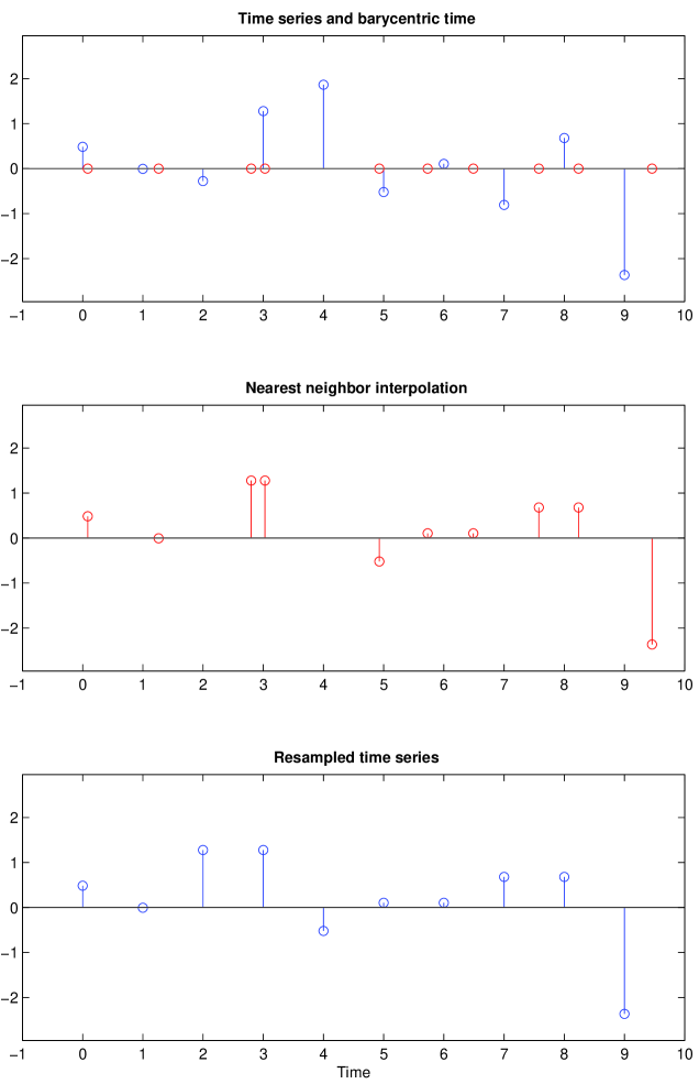
Thus to convert the integral (85) into a Fourier transform we need to resample the function $x(t)\,a(t)\,e^{-\mathrm{i}\phi_{\mathrm{s}}(t)}$ according to Eq. (86). We consider two numerical interpolation methods in order to obtain the resampled function. The first method is the nearest neighbor interpolation also called the stroboscopic resampling. We assume that the original data is a time series $x_{k}$ ($k=1,\ldots,N$), sampled at uniform intervals. In this method we obtain the value of the time series $x_{k}$ at barycentric time $t_{\mathrm{b}}$ by taking the value $y_{k_{0}}$ such that $k_{0}$ is the nearest integer to $t_{\mathrm{b}}$. We have illustrated the method in Fig. 3.

Figure 3: Illustration of the nearest neighbor resampling method. The top panel shows the uniformly sampled original data and the points of the barycentric time. The middle panel shows the interpolations of the original time series at the points of the barycentric time, obtained by the nearest neighbor method. The bottom panel shows the resampled time series which is the uniformly sampled barycentric time series form the middle panel.

The second method has two steps. The first step consists of obtaining a more finely sampled time series and the second step consists of interpolating the upsampled time series to the barycentric time using splines boor-78 . To perform the first step we use an interpolation method based on the Fourier transform. We take the Fourier transform of the original time series, pad the Fourier transform series with an appropriate amount of zeros and then transform it back to the time domain by inverse Fourier transform. The Fourier transforms are performed using the FFT algorithm. We thus obtain an interpolated time series with points inserted between the original points. If we have a time series with $N$ points and pad its discrete Fourier transform with $N$ zeros, by inverse transform we obtain a $2N$-point time series. The second step consists in applying splines to interpolate the upsampled time series to the barycentric time for number of points equal to the number of original data points. Thus if the original time series contains $N$ points the final interpolated time series contains also $N$ points.

We have compared the performance of the two interpolation methods and we have also compared these methods with an exact matched filter. To carry out the comparison we have used noise-free waveforms given in Eqs. (1)–(6) with one spin-down parameter. We have calculated the ${\mathcal{F}}$-statistic using the two interpolation methods and exact matched-filtering method. In the matched filtering method we have assumed that we know the frequency of the signal and thus the Doppler modulation due to the motion of the detector. However, we have used FFT to calculate the ${\mathcal{F}}$-statistic for the whole frequency band. The results are shown in Fig. 4.

Figure 4: Comparison of the two interpolation methods and the perfect matched-filtering. We see that the two-step interpolation method that uses Fourier and spline interpolation very accurately reproduces the perfect matched filter.

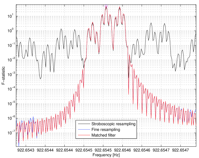
We have performed a Monte Carlo simulation consisting of 1000 trials and we have found that the rms error divided by maximum of the ${\mathcal{F}}$-statistic in the second method was $0.1\%$ whereas in the first, fastest method it was $5\%$. The nearest neighbor interpolation leads to a greater signal-to-noise ratio loss than spline interpolation and also, very importantly, to elevated sidelobes of the ${\mathcal{F}}$-statistic. In the presence of noise this can lead to a loss of the parameter estimation accuracy if the noise elevates the sidelobes above the main maximum. The stroboscopic resampling is much faster than the second two step method however the second method is much more accurate than the first.

VI.2 FFT interpolation

Using the FFT algorithm we can efficiently calculate the discrete Fourier transform (DFT) $X(k)$ ($k=1,\ldots,N$) of a time series $x_{\ell}$ ($\ell=1,\ldots,N$). We recall that $X(k)$ is given by the following expression

$$X(k)=\sum^{N}_{\ell=1}x_{\ell}e^{-2\pi\mathrm{i}(\ell-1)(k-1)/N},\quad k=1,\ldots,N.$$ (88)

The frequencies $(k-1)/N$ are called Fourier frequencies and DFT components calculated at Fourier frequencies are called Fourier bins. When the true frequency of a monochromatic signal does not coincide with one of the Fourier frequencies, the use of the FFT algorithm to evaluate the sum (88) leads a certain loss of signal-to-noise ratio. The greatest loss equal around 36.3% is when the true frequency is half way between the Fourier frequencies.

One way to improve this situation is to pad the time series of $N$ data points with $N$ zeros. This leads to DFT evaluated at twice as many points as the DFT of the original time series and the signal-to-noise loss is only 9.97%. However this procedure leads to evaluating twice as long FFT as the original ones and thus increases the computational time by more than a factor of two.

There exists an approximate interpolation procedure proposed by pulsar astronomers (see Chapter 7.3.3 in Ref. JKbook ), in which the DFT component in the middle of two Fourier frequencies is approximated by

$$X(k+1/2)\cong[X(k+1)-X(k)]/\sqrt{2}.$$ (89)

This interpolation method is called interbinning. One can show (see Fig. 7.3 in Ref. JKbook ) that the interpolation based on Eq. (89) leads to maximum loss of signal-to-noise ratio of 13%.

VI.3 Finding the maximum of the ${\mathcal{F}}$-statistic accurately

Figure 5: An illustration of the Nelder-Mead algorithm in two dimensions. We first evaluate the function to be minimized on an initial triangle. At each step of the search, a new point in or near the current triangle is generated. The function value at the new point is compared with the function’s values at the vertices of the triangle and, usually, one of the vertices is replaced by the new point, giving a new triangle. This step is repeated until the diameter of the simplex is less than the specified tolerance. In the method the triangle adapts itself to the local landscape, elongating down long inclined planes, changing direction on encountering a valley at an angle, and contracting in the neighborhood of a minimum.

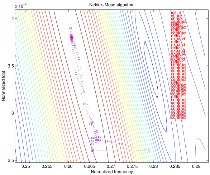
As we calculate the ${\mathcal{F}}$-statistic on a discrete grid in the parameter space and as the maximum of the ${\mathcal{F}}$-statistic does not in general coincide with a node of the grid, we always lose some signal-to-noise ratio and parameter estimation accuracy. To improve this we use a nonlinear optimization routine to find an improved maximum of our statistic.

The search for the maximum of the ${\mathcal{F}}$-statistic is performed in two steps. First we find the maximum of ${\mathcal{F}}$ over the discrete grid in the parameter space and then the parameters obtained in this coarse search we input as initial values to some hill-climbing optimization routine to find an improved maximum. The second step is called a fine search. As our maximum finding routine we can use a direct search that does not require calculations of derivatives of ${\mathcal{F}}$, namely the Nelder-Mead algorithm or simplex search algorithm nelder-65 . The Nelder-Mead algorithm is illustrated in Fig. 5 for two-dimensional case where simplices are triangles.

VII Monte Carlo simulations

We have implemented the data analysis methods presented in the previous sections in a computer code and we have performed a number of Monte Carlo simulations to test how accurately we can estimate signal’s parameters for different values of the signal-to-noise ratio (SNR) and how the rms errors of our ML estimators compare to the Cramèr-Rao lower bound. For unbiased estimators the Cramèr-Rao lower bound on variances of the estimators is given by the diagonal elements of the inverse of the Fisher matrix. The ML estimators are asymptotically (i.e. when SNR tends to infinity) unbiased and with variances approaching the diagonal elements of the inverse of the Fisher matrix. Our Monte Carlo simulations consisted of generating the data that were the sum of the white noise and the gravitational-wave signal presented in Sec. II and using the filtering procedure from Sec. III to detect the signal and estimate its parameters. We have taken the observation time equal to exactly 2 sidereal days. For this observation time it is enough to take only the first spin-down parameter in the templates (see Refs. BCCS98 ; JK00 ). To obtain the Cramèr-Rao lower bound we have calculated the $8\times 8$ Fisher matrix [defined in Eq. (38)] for the signal model given in Sec. II with one spin down parameter included.

We have made our simulation to mimic the analysis of the VIRGO interferometer VSR1 data. We have thus assumed that data comes from an interferometric detector located at the position of the VIRGO detector and we have used the detector’s ephemerides corresponding to data taken sometime in the year 2007. We have generated data in a narrow frequency band of 50 mHz with the lower edge of the band equal to 435.1875 Hz. This resulted in a short time series of 17233 data points greatly reducing the CPU time needed to perform the simulations. For all the simulations we have chosen the same parameters of the gravitational-wave signal except for the constant amplitude $h_{0}$ that we scaled to obtain data with a chosen SNR [defined in Eq. (37)]. We have found the grid point $p_{g}$ nearest to the true position of the signal in the parameter space and we have calculated the ${\mathcal{F}}$-statistic on a small grid around the point $p_{g}$. The size of the grid was $\pm 2$ grid points from the point $p_{g}$ in the direction of the parameters $\dot{\omega}$, $\alpha_{1}$, $\alpha_{2}$ [see Eqs. (33)]. For each set of these three parameters we have evaluated the ${\mathcal{F}}$-statistic for the whole 50 mHz band.

In all the simulations we have used the constrained grid constructed in Sec. IV and we have chosen the detection threshold for the ${\mathcal{F}}$-statistic equal to 10. This low threshold ensured that the probability of detection was nearly one and none of the signals was missed. In each simulation the estimation of signal’s parameters was performed in two steps. The first step, called the coarse search, was the calculation of the ${\mathcal{F}}$-statistic on the grid described in Sec. IV. We have registered all the threshold crossings and we have taken the coarse estimates of the signal’s parameters as the parameters of the grid point for which the ${\mathcal{F}}$-statistic was maximal. In the second step, called the fine search, we have found the maximum of the ${\mathcal{F}}$-statistic for each signal registered in the first step using the Nelder-Mead algorithm with the initial values equal to the coarse estimates of the parameters. In this step the ${\mathcal{F}}$-statistic was calculated [by means of Eqs. (30)–(31)] exactly without any approximations. For each value of the SNR we have repeated the simulation 1000 times with different realizations of the white Gaussian noise.

Figure 6: Standard deviations (left panels) and biases (right panels) of the ML estimators of the intrinsic parameters as functions of the SNR computed with the grid of $\mathrm{MM}=\sqrt[3]{0.9}$. The plots are made, from the top, for the following parameters: frequency, spin down, declination, and right ascension. Each circle corresponds to a standard deviation or a bias computed from simulation of 1000 runs. The continuous lines in the left panels are the Cramér-Rao bounds for standard deviations.

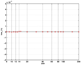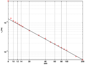
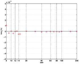
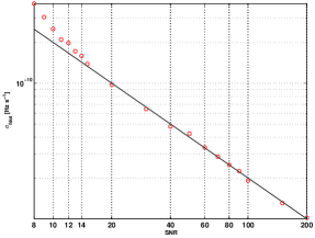
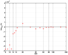
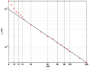
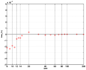
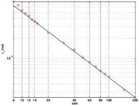
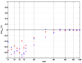
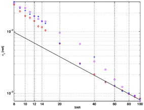
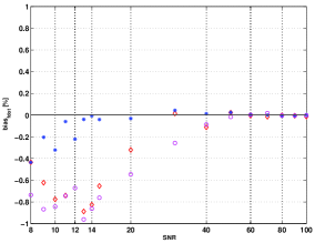
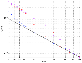
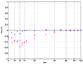
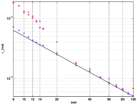
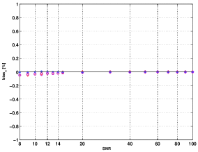
In the first simulation we have employed a fine grid with the minimal match $\mathrm{MM}=\sqrt[3]{0.9}$. We have used the accurate two-step resampling procedure described in Sec. VI.1 and before applying the FFT we have padded the data with 15535 zeros resulting in a time series of $2^{15}$ points. This ensured an exact interpolation of the DFT between the Fourier frequencies and the fastest implementation of the FFT algorithm (because the number of data points was a power of 2). The results of this simulation are presented in Fig. 6, where we have depicted standard deviations and biases of the intrinsic parameters of the signal: frequency, spin down, declination, and right ascension, as functions of the SNR. The results of simulation of 1000 runs are marked by the circles. Additionally in the left panels we have shown the Cramér-Rao bounds for the standard deviations calculated from the inverse of the Fisher information matrix. We see that for the SNRs greater than $\sim$9 the standard deviations obtained from simulation are very close to the Cramér-Rao bounds and the simulated biases are small fractions of a percent of the true values.

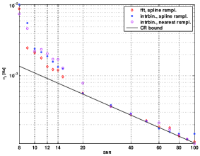
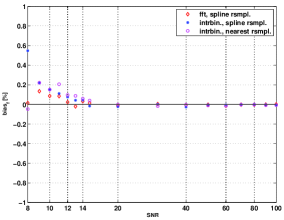
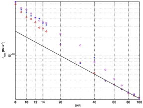
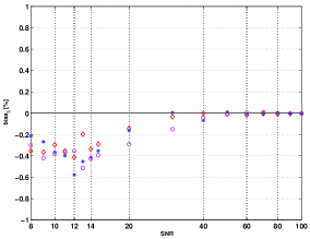
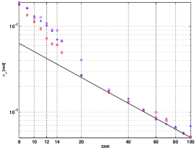
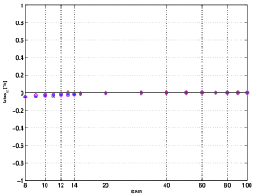
In the second simulation we have tested how accuracy of the parameter estimation is affected by various options of the algorithms described in the previous section. All these options aim at speeding up computations. In the simulation we were changing the thickness of the grid, we were comparing the two-step spline resampling with the nearest neighbor resampling, and we were also testing the interbinning interpolation [defined in Eq. (89)]. In all the runs we have used a thicker grid corresponding to the minimal match $\mathrm{MM}=\sqrt{3}/2$. We have studied three specific cases: (i) zero padding and spline interpolation; (ii) interbinning and spline interpolation; (iii) interbinning and the nearest neighbor interpolation. The results of the simulation are presented in Fig. 7. From comparison of the three cases it follows that with a coarser grid and with the use of different approximations the rms errors of the parameter estimators are greater but still at a reasonable level. In the range of the SNRs from $\sim$9 to $\sim$15, the standard deviations obtained from simulation are twice as large as the Cramér-Rao bounds, when we use spline resampling. For the nearest neighbor interpolation, for some parameters, the simulated rms error is twice as large as the Cramér-Rao bound for the SNRs up to $\sim$30.

Figure 7: Standard deviations (left panels) and biases (right panels) of the ML estimators of the intrinsic parameters as functions of the SNR computed with the grid of $\mathrm{MM}=\sqrt{3}/2$ for the following three cases: (i) zero padding and spline interpolation (diamonds); (ii) interbinning and spline interpolation (stars); (iii) interbinning and the nearest neighbor interpolation (circles). The continuous lines in the left panels are the Cramèr-Rao bounds.

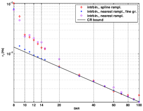
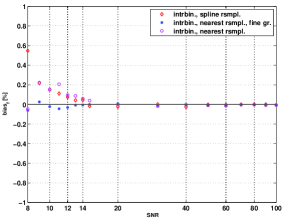
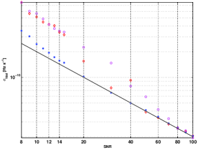
In the third simulation we have studied another three specific cases: (i) interbinning and spline interpolation, with a coarse grid of $\mathrm{MM}=\sqrt{3}/2$; (ii) interbinning with the nearest neighbor interpolation, with a fine grid of $\mathrm{MM}=\sqrt[3]{0.9}$; (iii) interbinning with the nearest neighbor interpolation, with a coarse grid of $\mathrm{MM}=\sqrt{3}/2$. The results of the simulation are presented in Fig. 8. This simulation shows that with a sufficiently fine grid even the use of the least accurate (but the fastest) resampling by the nearest neighbor interpolation leads to the rms errors of the intrinsic parameters very close to the Cramér-Rao bounds.

Figure 8: Standard deviations (left panels) and biases (right panels) of the ML estimators of the intrinsic parameters as functions of the SNR computed for the following three cases: (i) interbinning and spline interpolation, with the coarse grid of $\mathrm{MM}=\sqrt{3}/2$ (diamonds); (ii) interbinning with the nearest neighbor interpolation, with the fine grid of $\mathrm{MM}=\sqrt[3]{0.9}$ (stars); (iii) interbinning with the nearest neighbor interpolation, with the coarse grid of $\mathrm{MM}=\sqrt{3}/2$ (circles). The continuous lines in the left panels are the Cramèr-Rao bounds.