Model-independent cosmological constraints from the CMB

Abstract:

We analyse CMB data in a manner which is as independent as possible of the model of late-time cosmology. We encode the effects of late-time cosmology into a single parameter which determines the distance to the last scattering surface. We exclude low multipoles $\ell<40$ from the analysis. We consider the WMAP5 and ACBAR data. We obtain the cosmological parameters $100\omega_{{\mathrm{b}}}=2.13\pm 0.05$, $\omega_{{\mathrm{c}}}=0.124\pm 0.007$, $n_{s}=0.93\pm 0.02$ and $\theta_{A}=0.593^{\circ}\pm 0.001^{\circ}$ (68% C.L.). The last number is the angular scale subtended by the sound horizon at decoupling. There is a systematic shift in the parameters as more low $\ell$ data are omitted, towards smaller values of $\omega_{{\mathrm{b}}}$ and $n_{s}$ and larger values of $\omega_{{\mathrm{c}}}$. The scale $\theta_{A}$ remains stable and very well determined.

1 Introduction

The cosmic microwave background (CMB) is one of the most important cosmological probes. The pattern of acoustic oscillations of the baryon-photon plasma is imprinted on the CMB at the time of decoupling, and then rescaled (and on large scales modified) as the CMB photons propagate from the last scattering surface to the observer. The CMB is thus sensitive to cosmological parameters in two ways, via the physics at decoupling and via the evolution of the universe after that.

While the physics at decoupling –essentially atomic physics and general relativity of a linearly perturbed Friedmann-Lemaître (FL) universe– is well understood, the evolution at late times deviates from the predictions of linearly perturbed FL models with radiation and matter. The difference may be due to an exotic matter component with negative pressure such as vacuum energy, deviation of gravity from general relativity [5, 2, 4, 3], or a breakdown of the homogeneous and isotropic approximation [6, 7, 8, 9, 10, 11]. It is not known which of these possibilities is correct, and there are large differences between the various models. It is therefore worthwhile to analyse the CMB in a manner which is as independent of the details of late-time cosmology as possible. On the one hand, this clarifies the minimal constraints that all models of late-time cosmology, whatever their details, have to satisfy in order to agree with CMB observations. On the other hand, our analysis provides limits on the physical parameters at decoupling that are independent of the details of what happens at later times. This is particularly important for cosmological parameters such as the density of baryons, density of dark matter and the spectral index, which are used to constrain particle physics models of baryogenesis, supersymmetry and inflation, which are independent of late-time cosmology.

Such a separation of constraints is possible because the physics after decoupling affects the CMB in a rather limited manner (except at low multipoles), by simply changing the angular scale and modifying the overall amplitude of the CMB pattern. We encode the change in the angular scale in a single parameter related to the angular diameter distance to the last scattering surface and treat the amplitude as a nuisance parameter. We aim to be transparent about how the different cosmological parameters enter the calculation and the assumptions that go into the analysis.

In section 2 we discuss how the physics at early and late times affects the CMB and explain our assumptions. In section 3 we present the results of the analysis of the WMAP 5-year data [12, 13, 14] and the ACBAR data [15] and give the constraints on cosmological parameters. In section 4 we summarise our results. Some details are collected in two appendices.

2 Parameter dependence of the CMB

2.1 Our assumptions

The pattern of CMB anisotropies can be summarised in terms of a few parameters. It was noted in [16] that models with the same primordial perturbation spectra and same values of $\omega_{{\mathrm{b}}},\omega_{{\mathrm{c}}}$ and the shift parameter $R$ have an identical CMB spectrum today, apart from low multipoles ($\ell\lesssim 30$). The discussion in [16] was in the context of a family of Friedmann-Lemaître (FL) models, but the statement is true more generally. The shift parameter is defined as

$$R \equiv \omega_{\mathrm{m}}^{1/2}(1+z_{*})H_{0}h^{-1}D_{A}(z_{*})$$ (1)

$$= \left(\frac{\Omega_{m}}{\Omega_{K}}\right)^{1/2}\sinh\left(\Omega_{K}^{1/2}\int_{0}^{z_{*}}\mathrm{d}z^{\prime}\frac{H_{0}}{H(z^{\prime})}\right)\ ,$$

where $z_{*}$ is the redshift of decoupling, $D_{A}(z)$ is the angular diameter distance between today and redshift $z$, $H_{0}=100h$km/s/Mpc is the Hubble parameter today, and the second equation holds for all FL models. The density parameter $\omega_{{\mathrm{b}}}$ is the normalized dimensionless physical density of baryonic matter, $\omega_{{\mathrm{b}}}=8\pi G_{\mathrm{N}}\rho_{b}/3$/(100 km/s/Mpc)², $\omega_{{\mathrm{c}}}$ is the normalized dimensionless physical density of cold dark matter defined the same way, $\omega_{\mathrm{m}}=\omega_{{\mathrm{b}}}+\omega_{{\mathrm{c}}}$ is the total physical matter density, and $\Omega_{\mathrm{m}}=\omega_{\mathrm{m}}h^{-2}$ and $\Omega_{K}$ are, respectively, the matter and the spatial curvature density parameter today. With present observations which include polarization data, one has to add a parameter to take into account collisions between the CMB photons and baryonic matter after the cosmic medium becomes reionized. This is usually expressed with the redshift of reionization $z_{\mathrm{ri}}$ or the optical depth $\tau$.

The CMB data have been analysed in terms of the shift parameter $R$ in various FL models [17, 12, 18, 19, 20, 21, 22], and a similar approach has been followed for local void models [10, 23]. The model-dependence of parameters such as $R$ has been discussed, but limits on them have always been derived within some specific models, and it has not been clear which assumptions are important and what is the model-independent information.

In this work, we analyse the CMB in a manner which is as model-independent as possible, and we are explicit about the assumptions involved. In particular, we do not restrict our study to models which are close to FL at late times, so our constraints are also applicable to models where the effect of non-linear structures on the expansion rate is important, or where we are located in a large spherically symmetric density fluctuation such as a local void. (Note that the near-isotropy of the CMB does not imply that the universe is close to FL, even coupled with the Copernican principle [24].)

We assume that the physics up to and including decoupling is completely standard, i.e. linearly perturbed FL evolution according to normal four-dimensional general relativity with Standard Model particle physics and dark matter (which we assume to be cold during decoupling). As for physics after decoupling, we make the minimal assumptions that it changes the small angle CMB spectrum only by 1) modifying the angular diameter distance to the last scattering surface and 2) changing the overall amplitude. Here, small angles refers to scales which are well inside the horizon at late times when the unknown physics can be important, say conservatively at $z\,\raisebox{-2.58334pt}{$\buildrel<\over{\sim}$}\,60$. We discard low multipoles in our analysis, because typically the unknown physics of dark energy, modified gravity or large deviations from FL geometry affects the large angles in a model-dependent way, for example via the late Integrated Sachs-Wolfe (ISW) effect. In typical perturbed FL models, the late ISW effect is only significant at low multipoles (see appendix A), and the Rees-Sciama effect, gravitational lensing and the Sunyaev-Zel’dovich effect do not have a significant impact at the present observational accuracy [26, 27, 25], though their presence is already suggested by the ACBAR data [15]. We assume that such effects remain small in other models, and that any multipole-dependent effect of new physics on the CMB spectrum is below the observational precision, except at low multipoles.

In perturbed FL models, reionization has a significant effect on all angular scales, but at high multipoles it amounts to a simple rescaling of the amplitude, and is thus degenerate with the amplitude of primordial perturbations (see appendix B), so we can neglect modeling of reionization.

We assume that the primordial perturbations are adiabatic, and have a power-law spectrum. We only consider scalar perturbations, and assume that vector and tensor contributions are small. (This division refers to the early universe; in the late universe it is not necessarily meaningful, because we do not assume that the late universe is close to FL.) Within our approach it would not be easy to include tensor perturbations in the temperature anisotropy spectrum, because they contribute mainly via the ISW effect and are relevant up to $\ell\approx 100$. However, the contribution of tensors starts to decay already around $\ell\approx 50$ and is probably relatively small, so their presence would not be expected to change our results significantly. (It would be easy to take into account the tensor contribution to the polarization spectrum, though, because it is mainly generated at the last scattering surface.) We also neglect the effect of neutrino masses.

The idea behind these assumptions is that we can treat the CMB with a standard Boltzmann code, and simply exclude low multipoles from the analysis. We have modified the publicly available CAMB code and the corresponding Monte Carlo Markov Chain program [28] to search for best-fit values of our parameters. As long as the rise to the first peak is fully included in the analysis, discarding low multipoles should not involve a significant loss of information, because there are more high multipoles and the cosmic variance is larger on large scales. However, our results in this respect are somewhat surprising, as we discuss in section 3. Also, it has been argued that there are anomalies in the angular distribution on large scales [29] (and a dipolar modulation at higher multipoles [30]), which could indicate that some physics affecting the low multipoles is not understood, so they may be unreliable for cosmological analysis; see also [31, 32].

Our assumptions do not hold for models with non-standard physics at or before decoupling, such as new radiation degrees of freedom, early dark energy [33] or dark matter which undergoes significant annihilation at early times [34]. In models where we are located in a large spherically symmetric region, it is possible to obtain a large CMB dipole [35], and there could be a large effect at higher multipoles as well. This can only be checked with perturbation theory adapted to such models, which is now being developed [36].

2.2 The physics of the CMB parameters

Let us outline the relation between the features in the CMB spectrum and the cosmological parameters, given our assumptions above. (See [27, 37] for detailed discussion.) We consider five parameters, namely the overall amplitude, the baryon density $\omega_{{\mathrm{b}}}$, the cold dark matter density $\omega_{{\mathrm{c}}}$, the spectral index $n_{s}$ and the distance to the last scattering surface $D_{A}(z_{*})$.

The observed amplitude of CMB perturbations is determined by a combination of the primordial power spectrum and late-time physics, such as damping due to accelerating expansion and scattering of CMB photons from matter due to reionization. Without specifying a model for the late-time universe, it is not possible to disentangle these effects. Because the overall normalization does not have a model-independent interpretation, we treat it as a nuisance parameter, i.e., we marginalize over it and do not quote limits for it.

The spectral index $n_{s}$ is related to the early universe physics, such as inflation, which produces the primordial perturbations. Extending the analysis to more complicated primordial spectra would be straightforward, though of course we would not be sensitive to large-scale features.

The relative height and depth of the CMB peaks and troughs is set by the physics of the baryon-photon oscillations, which depends on $\omega_{{\mathrm{b}}}$ and $\omega_{{\mathrm{c}}}$. This pattern also depends on the radiation density $\omega_{r}=8\pi G_{\mathrm{N}}\rho_{r}/3$/(100 km/s/Mpc)², which is however accurately determined by the CMB temperature. Note that the CMB is only sensitive to the densities at the time of decoupling, not to their values today. As is customary, we use the symbols $\omega_{{\mathrm{b}}}$, $\omega_{{\mathrm{c}}}$ and $\omega_{r}$ to refer to the densities at decoupling scaled to today with the factor $(1+z_{*})^{3}$ for baryons and dark matter and $(1+z_{*})^{4}$ for radiation, where $*$ indicates the time of decoupling. At decoupling, the distribution of matter is still very smooth, so the densities at that time can be understood as local or average values; the scaled numbers represent today’s average values. In a statistically homogeneous and isotropic space, the mean energy density of baryons and cold dark matter evolves like $(1+z)^{3}$ due to conservation of mass, and the mean energy density of photons evolves like $(1+z)^{4}$ due to conservation of photon number and the fact that the change of energy of the CMB photons by scattering can be neglected [38]. FL models are of course a particular case of this. If dark matter has significant pressure, or decays significantly [39], or if there is some extra source of baryons, dark matter or photons, our $\omega_{{\mathrm{b}}},\omega_{{\mathrm{c}}}$ and $\omega_{r}$ would not correspond to the physical densities today. (Dark matter decay to radiation would also contribute to the late ISW effect [40].) This is already true for neutrinos, which we treat as massless, but which in fact do not contribute to the present-day radiation density, since their mass today is larger than the temperature. This will also be the case if the factor $(1+z)^{3}$ is not simply proportional to the volume, which can happen if statistical homogeneity and isotropy is broken, such as in local void models where shear can contribute significantly to the redshift.

Our final parameter is the angular diameter distance to the last scattering surface. The angular diameter distance out to redshift $z$ is defined as $D_{A}(z)=L/\theta$, where $L$ is the proper size of an object at redshift $z$ and $\theta$ is its observed angular size. The physical scale of the baryon-photon oscillations is set by the sound horizon at decoupling $r_{s}(z_{*})$ which depends on $\omega_{{\mathrm{b}}}$ and $\omega_{{\mathrm{c}}}$ [41, 27]. With standard physics up to decoupling, the sound speed of the photon-baryon plasma is

$$c_{s}^{2}=\frac{1}{3(1+3\rho_{b}/4\rho_{\gamma})}=\frac{1}{3\left(1+\frac{3\omega_{{\mathrm{b}}}}{(1+z)4\omega_{\gamma}}\right)}\equiv\frac{1}{3[1+r(1+z)^{-1}]}\ ,$$ (2)

where we have introduced $r\equiv 3\omega_{{\mathrm{b}}}/4\omega_{\gamma}$. For the sound horizon we obtain

$$(1+z_{*})r_{s}(z_{*}) = \int_{0}^{t_{*}}\frac{c_{s}(t^{\prime})}{a(t^{\prime})}dt^{\prime}$$ (3)

$$= \frac{h}{H_{0}\sqrt{3}}\int_{1+z_{*}}^{\infty}\frac{dx}{x\sqrt{(x+r)(x\omega_{r}+\omega_{\mathrm{m}})}}$$

$$= \frac{2h}{H_{0}\sqrt{3r\omega_{\mathrm{m}}}}\log\left(\frac{\sqrt{1+z_{*}+r}+\sqrt{\frac{(1+z_{*})r\omega_{r}}{\omega_{m}}+r}}{\sqrt{1+z_{*}}\left(1+\sqrt{\frac{r\omega_{r}}{\omega_{\mathrm{m}}}}\right)}\right)\ .$$

Note that $h/H_{0}=1/(100$km/s/Mpc$)\approx 2998$ Mpc is a fixed scale which does not depend on the cosmological model. The photon energy density $\omega_{\gamma}\approx 2.48\times 10^{-5}$ is known as well as the CMB temperature and we do not treat it as a free parameter. Assuming massless neutrinos, the same is true for the radiation density [27], $\omega_{r}=\omega_{\gamma}\left(1+3\frac{7}{8}\left(\frac{4}{11}\right)^{4/3}\right)\approx 4.17\times 10^{-5}.$ Furthermore, for standard radiation content, $z_{*}\approx 1090$ and it depends weakly on $\omega_{{\mathrm{b}}}$ and $\omega_{{\mathrm{c}}}$ (for an analytical approximation, see [41]). For standard values of the parameters, the log in (3) is of order unity. The sound horizon at decoupling therefore depends only on $\omega_{{\mathrm{b}}}$ and $\omega_{{\mathrm{c}}}$. The angle under which it is observed today is given by $\theta_{A}\equiv r_{s}(z_{*})/D_{A}(z_{*})$. With $\omega_{{\mathrm{b}}}$ and $\omega_{{\mathrm{c}}}$ fixed, the pattern of CMB anisotropies is determined at decoupling (apart from low multipoles), and its angular scale changes as the distance to the last scattering surface grows and the multipole positions of the CMB peaks and troughs scale with $D_{A}(z_{*})$. Given our assumptions, the CMB (apart from low multipoles) has no sensitivity to any physical parameters other than $\omega_{{\mathrm{b}}},\omega_{{\mathrm{c}}},n_{s},D_{A}$ and the overall amplitude, and these five parameters are a priori independent. A given model can of course couple them to each other, as well as to parameters which do not directly affect the CMB.

In particular, in linearly perturbed FL models the spatial curvature affects the CMB only via the angular diameter distance (apart from the late ISW effect). It is sometimes said that the spatial curvature can be determined from CMB observations by using the sound horizon as a standard ruler (assuming that the universe can be described by a FL model). However, as (1) shows, the effect of spatial curvature on $D_{A}(z_{*})$ is completely degenerate with the expansion history $H(z)$. For example, FL models with matter and significant spatial curvature are consistent with the WMAP observations [42]. In that case, a prior on $H_{0}$ is enough to exclude large spatial curvature, but only because of the specific form of the expansion history. The only way to really measure the spatial curvature, as opposed to doing parameter estimation in the context of specific models, is to use independent observations of the distance and expansion rate [43], such as from the ages of passively evolving galaxies [44] and baryon acoustic oscillations [45]. Note also that the CMB (apart from low multipoles) is sensitive to the expansion history between decoupling and today only via the angular diameter distance; in particular, the CMB contains no model-independent information about $H_{0}$.

In addition to $R$, another parameter defined as

$$\ell_{A}\equiv\frac{\pi}{\theta_{A}}=\pi\frac{D_{A}(z_{*})}{r_{s}(z_{*})}$$ (4)

has also been introduced to parametrise the distance to the last scattering surface [46]. The parameter $\ell_{A}$ is related to the position of the first peak in multipole space (for details, see [27, 37, 46, 47]). The quantity $\ell_{A}$ has been called an independent shift parameter in addition to $R$ [19]. However, this is somewhat misleading, because $R$ and $\ell_{A}$ contain the same information as regards the shift in the angular scale of the CMB anisotropy pattern due to the late-time evolution, the only difference is their dependence on $\omega_{{\mathrm{b}}}$ and $\omega_{{\mathrm{c}}}$. Of course, one can consider any combination of the four parameters $\omega_{{\mathrm{b}}},\omega_{{\mathrm{c}}},n_{s}$ and $R$. For our purposes, it is useful to introduce the scale parameter $S$, which is defined as the ratio of the angular diameter distance to the prediction of the simplest cosmological model,

$$S \equiv \frac{D_{A}(z_{*})}{D_{A,EdS}(z_{*})}=\frac{H_{0}(1+z_{*})D_{A}(z_{*})}{2[1-(1+z_{*})^{-1/2}]}\simeq\frac{1}{2}H_{0}(1+z_{*})D_{A}(z_{*})\ ,$$ (5)

where $D_{A,EdS}$ is the angular diameter distance in the Einstein-de Sitter (EdS) universe (the matter-dominated spatially flat FL model), $(1+z)D_{A,EdS}=2H_{0}^{-1}[1-(1+z)^{-1/2}]$; the last approximation in (5) is accurate to 3%. Using (1), the scale parameter $S$ is related to $R$ by $S=hR/(2\omega_{\mathrm{m}}^{1/2})[1-(1+z_{*})^{-1/2}]^{-1}\simeq hR/(2\omega_{\mathrm{m}}^{1/2})$. Unlike $R$ and $\ell_{A}$, the scale parameter $S$ depends on the Hubble parameter, to which the CMB has no direct sensitivity. (This arises because FL models predict the distance in units of $H_{0}$.) Therefore, the value of $S$ depends on how we fix the Hubble parameter.

We can simply keep $H_{0}$ free and quote limits for $h^{-1}S$, and one can then substitute the Hubble parameter given by e.g. local observations of $H_{0}$. The mean value is $h^{-1}S=2.4$ (see table 2), so for $h=$ 0.6–0.7, the distance to the last scattering surface is a factor of 1.4–1.7 longer than in an EdS model with the observed Hubble parameter. This is in accordance with the usual intuition that physics in the late-time universe acts to increase the distance compared to EdS, for example via accelerated expansion. We could instead keep the age of the universe fixed, i.e. ask how large the distance is compared to the value in an EdS model at the same time after the big bang. In an EdS model $H_{0}=2/(3t_{0})$, so we have $S=2/(3t_{0}100\mathrm{km/s/Mpc})\times R/(2\omega_{\mathrm{m}}^{1/2})[1-(1+z_{*})^{-1/2}]^{-1}$, which for $t_{0}=13.4$ Gyr [48] gives $S\approx 1.2$ for our mean values $\omega_{\mathrm{m}}=0.145$ and $R=1.77$.

Finally, we can ask how long the distance is compared to an EdS model which has the correct matter density. The Hubble parameter is then simply $h=\omega_{\mathrm{m}}^{1/2}$, so $S=R/2[1-(1+z_{*})^{-1/2}]^{-1}\simeq R/2\approx 0.9$. This means that in an EdS model with the correct matter density, the predicted distance to the last scattering surface is longer than observed. (In other words, the real matter density decays faster as function of the distance to the last scattering surface than in the EdS reference model.) Unless otherwise noted, we follow this last convention, and compare with an EdS model which has the correct matter density, at the expense of the age of the universe and the Hubble parameter. We give constraints for $\theta_{A},\ell_{A},R$, $S$, $h^{-1}S$, and $D_{A}(z_{*})$ in section 3. For fixed $\omega_{{\mathrm{b}}}$, $\omega_{{\mathrm{c}}}$ and $n_{s}$, these quantities contain the same information, only their correlation properties with the parameters $\omega_{{\mathrm{b}}}$, $\omega_{{\mathrm{c}}}$ and $n_{s}$ are different (see table 3).

2.3 The distance to the last scattering surface

Let us now study how the CMB spectrum depends on the angular diameter distance to the last scattering surface $D_{A}(z_{*})$. We consider two positions on the sky denoted by $\boldsymbol{n}_{1}$ and $\boldsymbol{n}_{2}$ which have the temperature fluctuations $\Delta T(\boldsymbol{n}_{1})$ and $\Delta T(\boldsymbol{n}_{2})$ and which are separated by proper distance $L$ on the last scattering surface. For two different angular diameter distances $D_{A}$ and $D_{A}^{\prime}$ to the last scattering surface, the length $L$ is seen under the angles $\theta=L/D_{A}$ and $\theta^{\prime}=L/D^{\prime}_{A}$, see figure 1.

Figure 1: The angle under which two fixed points on the sky are seen changes with the angular diameter distance $D_{A}$.

The two-point functions ${\mathcal{C}}$ and ${\mathcal{C}}^{\prime}$ which correlate $\boldsymbol{n}_{1}$ and $\boldsymbol{n}_{2}$ for an observer at distance $D_{A}$ or $D_{A}^{\prime}$, respectively, can be decomposed in terms of the two angles as

$${\mathcal{C}}(\theta)\equiv\langle\Delta T(\boldsymbol{n}_{1})\Delta T(\boldsymbol{n}_{2})\rangle = \frac{1}{4\pi}\sum_{\ell}(2\ell+1)C_{\ell}P_{\ell}(\cos\theta)$$ (6)

$$= \frac{1}{4\pi}\sum_{\ell}(2\ell+1)C^{\prime}_{\ell}P_{\ell}(\cos\theta^{\prime})={\mathcal{C}}^{\prime}(\theta^{\prime})\,,$$

where $P_{\ell}$ is the Legendre polynomial of degree $\ell$, and $C_{\ell}$ and $C^{\prime}_{\ell}$ are the power spectra corresponding to the angular diameter distances $D_{A}$ and $D_{A}^{\prime}$ respectively. The equality ${\mathcal{C}}(\theta)={\mathcal{C}}^{\prime}(\theta^{\prime})$ means that we consider only correlations on the last scattering surface (or very close to it) and neglect line-of-sight effects like, e.g. the late ISW effect which can be different for the two photon paths. Using the orthogonality of the Legendre polynomials, $\int_{-1}^{1}P_{\tilde{\ell}}(\mu)P_{\ell}(\mu)d\mu=2\delta_{\ell,\tilde{\ell}}/(2\ell+1)$, we obtain the relation

$$C_{\ell}=\sum_{\tilde{\ell}}\frac{2\tilde{\ell}+1}{2}C^{\prime}_{\tilde{\ell}}\int_{0}^{\pi}\sin\theta d\theta P_{\tilde{\ell}}[\cos(\theta D_{A}/D_{A}^{\prime})]P_{\ell}(\cos\theta)\ .$$ (7)

This cumbersome exact expression is only needed for low values of $\ell$. At high $\ell$ we can work in the flat sky approximation (see [27], section 5.4), where

$$Y_{\ell m}\rightarrow\frac{1}{2\pi}\exp(i{\boldsymbol{\ell}}\cdot\boldsymbol{x})\quad\mbox{ and }P_{\ell}(\cos\theta)\rightarrow J_{0}(|\boldsymbol{x}|\ell)\ .$$

Here $\boldsymbol{x}$ is a vector on the flat sky, $\boldsymbol{\ell}$ is the variable of its 2-dimensional Fourier transform, with $\ell=|\boldsymbol{\ell}|$, and $J_{0}$ is the Bessel function of order $0$. Denoting $r\equiv|\boldsymbol{x}|$, the correlation function is

$${\mathcal{C}}(\theta)={\mathcal{C}}(r)=\frac{1}{2\pi}\int_{0}^{\infty}\!\!d\ell\,\ell J_{0}(r\ell)C_{\ell}\ .$$ (8)

The correlation functions corresponding to the two angular diameter distances are related by ${\mathcal{C}}(r)={\mathcal{C}}^{\prime}(r^{\prime})$, where $r^{\prime}=rD_{A}/D^{\prime}_{A}$,

$$\frac{1}{2\pi}\int_{0}^{\infty}\!\!d\ell\,\ell J_{0}(r\ell)C_{\ell} = \frac{1}{2\pi}\int_{0}^{\infty}\!\!d\ell\,\ell J_{0}(r^{\prime}\ell)C^{\prime}_{\ell}$$ (9)

$$= \frac{1}{2\pi}\left(\frac{D^{\prime}_{A}}{D_{A}}\right)^{2}\int_{0}^{\infty}\!\!d\ell\,\ell J_{0}(r\ell)C^{\prime}_{\frac{D_{A}^{\prime}}{D_{A}}\ell}\ ,$$

where on the second line we have simply performed the change of variables $\ell\rightarrow\ell D_{A}/D^{\prime}_{A}$. Using the property $\int_{0}^{\infty}rdrJ_{0}(r\ell)J_{0}(r\ell^{\prime})=\ell^{-1}\delta(\ell-\ell^{\prime})$, we obtain

$$C_{\ell} = \left(\frac{D_{A}^{\prime}}{D_{A}}\right)^{2}C^{\prime}_{\frac{D_{A}^{\prime}}{D_{A}}\ell}\ .$$ (10)

The relation (10) is valid independent of spatial curvature, since we do not invoke three-dimensional Fourier transforms. We are simply using the fact that the CMB anisotropies are functions on a sphere. This result agrees with [49] where it is derived in a different way and contrasts with [23], where there is an extra power of $D_{A}^{\prime}/D_{A}$. Let us denote the spectrum of a reference EdS Universe by $C_{\ell}^{EdS}$ and the measured CMB spectrum by $C_{\ell}$. Recalling the definition (5) of the scale parameter $S$, we can assign $C_{\ell}$ to an EdS universe with the same values of $\omega_{{\mathrm{b}}}$, $\omega_{{\mathrm{c}}}$ and $n_{s}$ and the angular diameter distance $D_{A}=SD_{A,EdS}$ if we scale the angular power spectrum by

$$C_{\ell}=S^{-2}C_{S^{-1}\ell}^{EdS}\ .$$ (11)

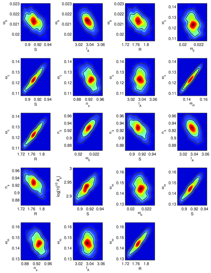
The basic assumption here is that the CMB fluctuations at decoupling are the same for both models and the only difference is the distance to the last scattering surface. If this is true, the relation (11) is exact in the flat sky limit. Without the flat sky approximation it has to be replaced by (7) with $D_{A}/D_{A}^{\prime}=S$. Note that despite of the factor $S^{-2}$ in (11), the shift parameter $S$ is not strongly correlated with the amplitude, it just shifts the spectrum in angular space. This is visible on the 2D-plots shown in Fig. 4. We have tested the flat sky approximation numerically and have found that for $\ell\geq 20$ the difference between (11) and the exact expression (7) is smaller than 1% for $1.1\geq S\geq 0.7$, which includes the region which is of interest to us (the mean value we obtain is $S=0.91\pm 0.01$, see table 2).

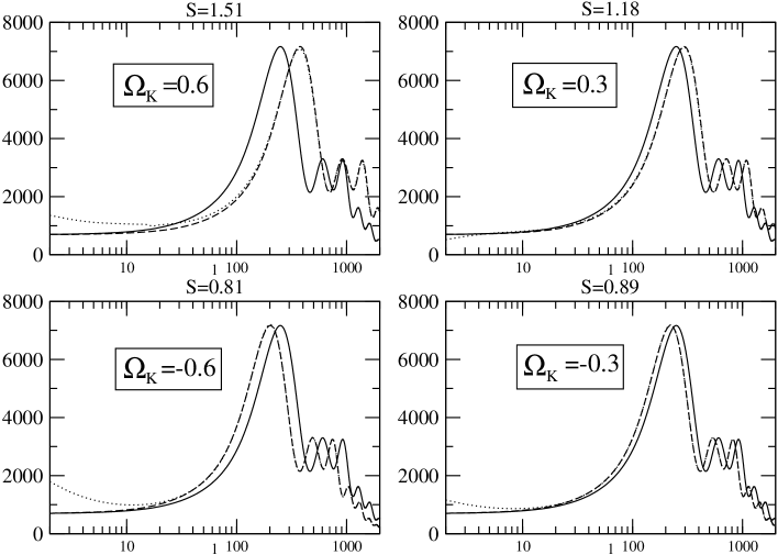
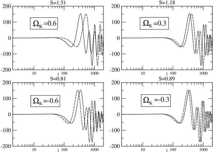
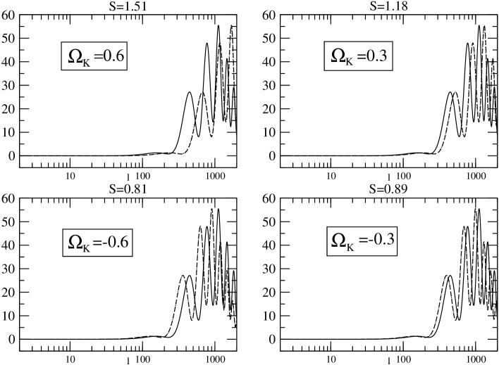
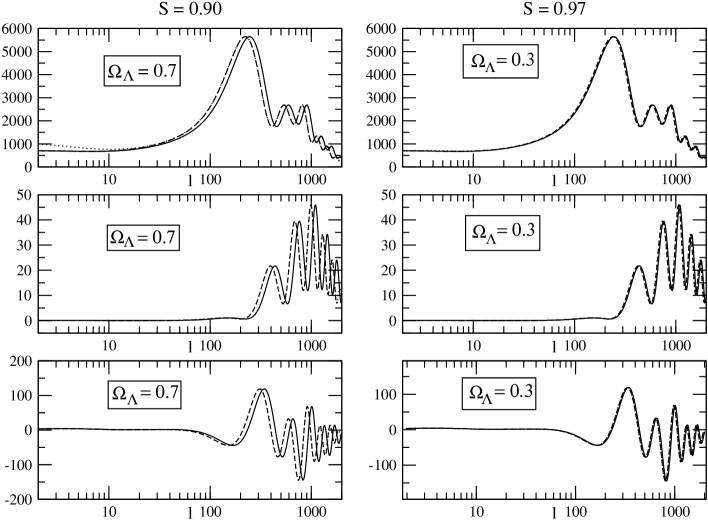
To illustrate the dependence of the CMB spectra on the scale parameter $S$, we show in appendix A the TT, TE and EE spectra for FL models with non-zero spatial curvature or cosmological constant, compared with the EdS result scaled with $S$. As shown in figures 5 to 7, the spectra for the scaled model and the model with spatial curvature lie on top of each other for $\ell\gtrsim 20$, except for the case of large negative spatial curvature with $S\approx 1.5$, where there is some difference in the TT spectra until $\ell\approx 100$. For the cosmological constant case, shown in figure 8, the approximation is excellent for all of the spectra for $\ell\gtrsim 20$.

3 Results

3.1 Cosmological parameters and the multipole cut

We use the WMAP5 data and the ACBAR data in our analysis. However, disregarding ACBAR does not change the results much. We have performed a Markov Chain Monte Carlo analysis with chain length $N=2\times 10^{5}$. The results change by significantly less than $1\sigma$ when going from $N=1.5\times 10^{5}$ to $2\times 10^{5}$, which indicates that the chains have converged well [28]. As a convergence test, we have checked that when the samples are split in two or three parts, the change of the relevant cosmological parameters is a few percent of one standard deviation. We have also checked that the Raftery and Lewis convergence diagnostic is satisfied [50].

$\ell_{\mathrm{min}}$	2	20	40	60
$100\omega_{{\mathrm{b}}}$	$2.21^{+0.05}_{-0.05}$	$2.19^{+0.05}_{-0.05}$	$2.18^{+0.07}_{-0.07}$	$2.15^{+0.08}_{-0.08}$
$\omega_{{\mathrm{c}}}$	$0.113^{+0.005}_{-0.005}$	$0.115^{+0.006}_{-0.006}$	$0.118^{+0.007}_{-0.007}$	$0.120^{+0.008}_{-0.008}$
$n_{s}$	$0.95^{+0.01}_{-0.01}$	$0.95^{+0.01}_{-0.01}$	$0.94^{+0.02}_{-0.02}$	$0.93^{+0.02}_{-0.02}$
$\Omega_{\Lambda}$	$0.72^{+0.03}_{-0.03}$	$0.71^{+0.04}_{-0.03}$	$0.70^{+0.04}_{-0.04}$	$0.68^{+0.06}_{-0.05}$
$\ell_{\mathrm{min}}$	80	100	120	140
$100\omega_{{\mathrm{b}}}$	$2.09^{+0.10}_{-0.10}$	$2.05^{+0.09}_{-0.09}$	$2.11^{+0.13}_{-0.12}$	$2.07^{+0.14}_{-0.14}$
$\omega_{{\mathrm{c}}}$	$0.127^{+0.012}_{-0.013}$	$0.132^{+0.012}_{-0.012}$	$0.126^{+0.013}_{-0.016}$	$0.131^{+0.018}_{-0.017}$
$n_{s}$	$0.91^{+0.03}_{-0.04}$	$0.89^{+0.04}_{-0.03}$	$0.91^{+0.05}_{-0.04}$	$0.90^{+0.05}_{-0.06}$
$\Omega_{\Lambda}$	$0.62^{+0.09}_{-0.09}$	$0.58^{+0.10}_{-0.09}$	$0.63^{+0.11}_{-0.10}$	$0.58^{+0.14}_{-0.14}$

Table 1: The change in the mean parameters when more low $\ell$ data are omitted, in the $\Lambda$CDM model with $\tau=0$. We have used the WMAP5 and ACBAR data.

In table 1 we show the effect of excluding a successively larger multipole range up to $\ell_{\mathrm{min}}$ in the analysis of the $\Lambda$CDM model; $\Omega_{\Lambda}$ is the vacuum energy density today, as usual. We have set $\tau=0$ for consistency with the treatment of the scaled model. From $\ell_{\mathrm{min}}=2$ to $\ell_{\mathrm{min}}=40$ the errors on $\omega_{{\mathrm{b}}}$ and $\omega_{{\mathrm{c}}}$ increase by 28%, while the error on $n_{s}$ increases by 57%. The central values move only by 1%, 4% and 1%, respectively, and the results are consistent within $1\sigma$.

Nevertheless, there is a systematic trend that $\omega_{{\mathrm{b}}}$ and $n_{s}$ decrease and $\omega_{{\mathrm{c}}}$ increases as $\ell_{\mathrm{min}}$ grows. Even at $\ell_{\mathrm{min}}=100$, where the shifts are maximized, they are less than $2\sigma$ in terms of the new error bars. In terms of the error bars of the model with $\ell_{\mathrm{min}}=2$, the shift is of course larger: for $n_{s}$ it more than 5$\sigma$, and for $\Omega_{\Lambda}$ more than 4$\sigma$. The feature that the error bars on $n_{s}$ increase more than those of $\omega_{{\mathrm{b}}}$ and $\omega_{{\mathrm{c}}}$ may be related to the fact that as $\ell_{\mathrm{min}}$ grows, the pivot scale $k=0.05$ Mpc^-1 moves closer to the edge of the data [51].

Part of this shift is due to the fact that reionization is neglected. We know from the absence of the Gunn-Peterson trough in quasar spectra that the Universe is reionized at redshifts $z\,\raisebox{-2.58334pt}{$\buildrel<\over{\sim}$}\,6$, see [52]. The slight decrease towards smaller scales which is usually attributed to reionization is now achieved with a somewhat redder spectrum. In order not to decrease the height of the acoustic peaks, this leads to a higher value of $\omega_{{\mathrm{c}}}$. A redder spectrum also enhances the amplitude difference between the well measured first and second peaks. This can be compensated by a reduction of $\omega_{{\mathrm{b}}}$, since a larger $\omega_{{\mathrm{b}}}$ means a larger difference between the odd contraction and even expansion peaks [27].

However, we have found that reionization is not the dominant effect, the systematic shift is also present if reionization is included in the analysis. We have checked this by including $\tau$ as a model parameter. The results of table 1 remain valid for also in this case. The problem is that for $\ell_{\min}\geq 40$ the value of $\tau$ is degenerate with a renormalization of the amplitude (see discussion in Appendix B) and the best fit value for $\tau$ fluctuates significantly from chain to chain. We therefore prefer to show the results for $\tau=0$. Note that the change is larger than the increase in the error bars. The shape of the one-dimensional probability distribution for the parameters is not for the most part significantly distorted, and the two-dimensional distributions do not show strong changes in the correlation properties as $\ell_{\mathrm{min}}$ increases. Therefore, the error bars do accurately represent the statistical error even at high $\ell_{\mathrm{min}}$. In other words, the shift in the parameters is systematic, and is not reflected in the statistical error estimate.

Figure 2: The increase in the large-scale power with increasing $\ell_{\mathrm{min}}$ in the best-fit $\Lambda$CDM models with $\tau=0$. The lowest line corresponds to a cut at $\ell_{\min}=2$ the subsequent lines have $\ell_{\min}=40,~{}60,~{}80$ and $100$, respectively. At $\ell_{\min}=120$ the large scale power no longer increases but it decreases somewhat. The WMAP and ACBAR data are superimposed. The vertical axis is $\ell(\ell+1)C^{TT}/(2\pi)$ in $(\mu K)^{2}$.

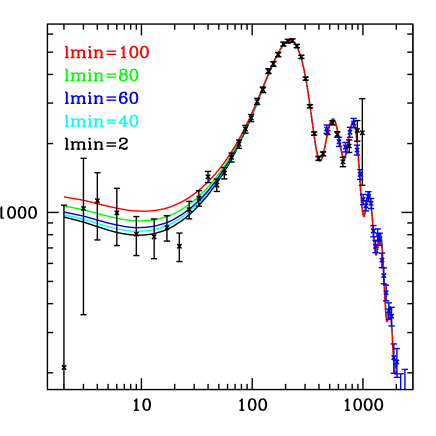
We conclude that the high $\ell$ data prefer different parameter values than the data which include the low multipoles. In figure 2 we show the TT power spectra for the best-fit $\Lambda$CDM models with different $\ell_{\mathrm{min}}$. There is a trend of increasing large-scale power with higher $\ell_{\mathrm{min}}$. In all cases, the overall amplitude is fixed well by the high $\ell$ data, and the effect is due to the change in $\omega_{{\mathrm{b}}},\omega_{{\mathrm{c}}}$ and $n_{s}$. We have checked that the ISW effect is not the cause: there is a similar shift for both the $\Lambda$CDM model and the scaled EdS model. Also, increasing $\ell_{\mathrm{min}}$ corresponds to decreasing $\Omega_{\Lambda}$ and hence a smaller contribution of the ISW effect to the low multipoles.

3.2 Model-independent parameter estimates

We fix our multipole cut at $\ell_{\mathrm{min}}=40$, which roughly corresponds to neglecting modes which entered the horizon after $z=60$. The dependence on the redshift is weak, $\ell_{\mathrm{min}}\propto(1+z)^{1/2}$ for $z\gg 1$. Choosing $z=30$ instead would give $\ell_{\mathrm{min}}\approx 30$. The cut at $\ell_{\mathrm{min}}=40$ is also motivated by the fact that for $\ell>40$ reionization is well approximated by a simple rescaling of the amplitude, as well as by the multipole dependence of the late ISW effect, see appendices A and B.

Parameter	Scaled	$\Lambda$CDM	$\Lambda$CDM
	$\ell_{\mathrm{min}}=40$	$\ell_{\mathrm{min}}=40$	$\ell_{\mathrm{min}}=2$
	mean	mean	mean
$100\omega_{{\mathrm{b}}}$	$2.13\pm 0.05$	$2.21\pm 0.07$	$2.24\pm 0.05$
$\omega_{{\mathrm{c}}}$	$0.124\pm 0.007$	$0.113\pm 0.007$	$0.111\pm 0.005$
$n_{s}$	$0.93\pm 0.02$	$0.96\pm 0.02$	$0.97\pm 0.01$
$S$	$0.91\pm 0.01$	–	–
$\Omega_{\Lambda}$	–	$0.72\pm 0.04$	$0.74\pm 0.03$
$\tau$	–	$0.09^{+0.04}_{-0.05}$	$0.09\pm 0.02$
$\omega_{m}$	$0.145\pm 0.007$	$0.136\pm 0.007$	$0.133\pm 0.005$
$h^{-1}S$	$2.40\pm 0.03$	–	–
$R$	$1.77\pm 0.02$	$1.73\pm 0.02$	$1.72\pm 0.02$
$\theta_{A}$	$0.593^{\circ}\pm 0.001^{\circ}$	$0.594^{\circ\,+0.002^{\circ}}_{\ \,-0.001^{\circ}}$	$0.593^{\circ}\pm 0.002^{\circ}$
$\ell_{A}$	$303.7\pm 0.7$	$303.3\pm 0.8$	$303.2\pm 0.7$
$D_{A}(z_{*})$/Mpc	$12.7\pm 0.2$	$12.9\pm 0.2$	$13.0\pm 0.1$
$r_{s}(z_{*})$/Mpc	$0.132\pm 0.002$	$0.134\pm 0.002$	$0.134\pm 0.001$
$10^{-3}z_{\mathrm{eq}}$	$3.5\pm 0.2$	$3.3\pm 0.2$	$3.2\pm 0.1$
$z_{*}$	$1094\pm 1$	$1092\pm 1$	$1091\pm 1$

Table 2: The mean values for the scaled model and the $\Lambda$CDM model. We have used the WMAP5 and ACBAR data for $\ell\geq\ell_{\mathrm{min}}=40$.

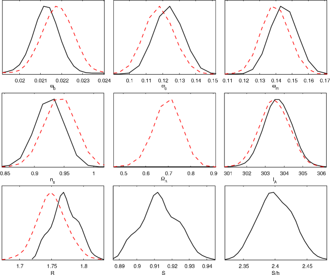
In table 2 we give the mean values for our primary parameters $\omega_{{\mathrm{b}}}$, $\omega_{{\mathrm{c}}}$, $n_{s}$ and $S$, as well as some derived parameters. In addition to the systematic effect discussed above, this table is our main result. As already mentioned, the overall amplitude is treated as a nuisance parameter. For comparison, we give the corresponding results for the $\Lambda$CDM model, with non-zero $\tau$. We use $\ell_{\mathrm{min}}=40$ in both cases. The $\Lambda$CDM values are in good agreement with the WMAP5 results [13] and have comparable error bars. For the scaled model, the errors in $\omega_{{\mathrm{c}}}$ and $n_{s}$ are slightly larger than those of the $\Lambda$CDM model with $\ell_{\min}=2$. We attribute this to the fact that we start at $\ell_{\mathrm{min}}=40$. Furthermore, our spectral index is somewhat redder, $n_{s}=0.93$ compared to $n_{s}=0.96$. This shift is also clearly seen in the one-dimensional likelihood functions for the scaled model and the $\Lambda$CDM model, shown in figure 3. However, these parameter changes are within one standard deviation and are therefore not statistically significant. It is impressive how accurately present CMB data determine $\ell_{A}$. The relative error is less than 0.3% for both the scaled model and $\Lambda$CDM. The error in the other parameters related to the angular diameter distance, $S,h^{-1}S,R$ and $D_{A}$, as well as $r_{s}$, is about 1%. The errors for $\omega_{{\mathrm{b}}},\omega_{{\mathrm{c}}}$ and $n_{s}$ are less than 3%, 6% and 2%, respectively.

In table 3 we give the covariance matrix between the different variables, and in figure 4 we show selected two-dimensional likelihoods. We see that $R$ and $S$ are strongly positively correlated with $\omega_{{\mathrm{c}}}$ and $\omega_{\mathrm{m}}$. In contrast, $D_{A}$ is strongly anti-correlated with $\omega_{{\mathrm{c}}}$ and $\omega_{\mathrm{m}}$. This can be understood by writing $D_{A}=SD_{A,EdS}$ and noting that $D_{A,EdS}\propto h^{-1}=\omega_{\mathrm{m}}^{-1/2}$. The variable $\ell_{A}$ is nearly uncorrelated with $\omega_{\mathrm{m}}$, but it is quite correlated with $\omega_{{\mathrm{b}}}$ and correspondingly also with $n_{s}$. Since most of the statistical weight of the WMAP data come from the first and second peaks, $n_{s}$ and $\omega_{{\mathrm{b}}}$ are strongly correlated even if the full WMAP data (with $\ell_{\mathrm{min}}=2$) are taken into account [12]. This correlation becomes stronger as some of the low $\ell$ data are omitted.

The standard deviations for the scaled EdS model are somewhat smaller than those of the $\Lambda$CDM model for the same $\ell_{\mathrm{min}}$. However, this does not mean that the fit is better, only that the well-fitting region is somewhat smaller. Error bars for a model can be small simply because different parts of the data prefer different regions of parameter space, so that the fit is good only in some small overlap region. In the present case, the scaled model and the $\Lambda$CDM model are comparably good fits to the data for $\ell_{\mathrm{min}}\geq 20$. In table 4 we show $-2\log{\cal L}$, where ${\cal L}$ is the likelihood of the best-fit, as a function of $\ell_{\mathrm{min}}$. There are only differences of $\approx 1$ in $-2\log{\cal L}$, which is the same order as the differences between different chains of the same model.

	$\omega_{{\mathrm{b}}}$	$\omega_{{\mathrm{c}}}$	$n_{s}$	$S$	$\omega_{\mathrm{m}}$	$h^{-1}S$	$\ell_{A}$	$D_{A}(z_{*})$	$r_{s}(z_{*})$	$z_{*}$
$\scriptsize{\omega_{{\mathrm{b}}}}$	$1.00$	$-0.31$	$0.84$	$-0.49$	$-0.23$	$-0.06$	$-0.56$	$0.02$	$0.14$	$-0.88$
$\omega_{{\mathrm{c}}}$	$-0.31$	$1.00$	$-0.51$	$0.96$	$1.00$	$-0.91$	$0.05$	$-0.94$	$-0.98$	$0.72$
$n_{s}$	$0.84$	$-0.51$	$1.00$	$-0.65$	$-0.45$	$0.19$	$-0.51$	$0.26$	$0.38$	$-0.86$
$S$	$-0.49$	$0.96$	$-0.65$	$1.00$	$0.94$	$-0.78$	$0.30$	$-0.82$	$-0.91$	$0.83$
$\omega_{\mathrm{m}}$	$-0.23$	$1.00$	$-0.45$	$0.94$	$1.00$	$-0.94$	$-0.004$	$-0.96$	$-1.00$	$0.66$
$h^{-1}S$	$-0.06$	$-0.91$	$0.19$	$-0.78$	$-0.94$	$1.00$	$0.32$	$1.00$	$0.96$	$-0.40$
$\ell_{A}$	$-0.56$	$0.05$	$-0.51$	$0.30$	$-0.004$	$0.32$	$1.00$	$0.27$	$0.06$	$0.43$
$D_{A}(z_{*})$	$0.02$	$-0.94$	$0.26$	$-0.82$	$-0.96$	$1.00$	$0.27$	$1.00$	$0.98$	$-0.47$
$r_{s}(z_{*})$	$0.14$	$-0.98$	$0.38$	$-0.91$	$-1.00$	$0.96$	$0.06$	$0.98$	$1.00$	$-0.58$
$z_{*}$	$-0.88$	$0.72$	$-0.86$	$0.83$	$0.66$	$-0.40$	$0.43$	$-0.47$	$-0.58$	$1.00$

Table 3: The normalized covariance matrix for the scaled model. We have used the WMAP5 and ACBAR data for $\ell\geq\ell_{\mathrm{min}}=40$. At this level of precision, the correlation coefficients of $R$ are the same as those of $S$, and those of $\theta_{A}$ are minus those of $\ell_{A}$.

Figure 3: One-dimensional likelihoods for the scaled model (black, solid) and the $\Lambda$CDM model (red, dashed). We have used the WMAP5 and ACBAR data for $\ell\geq\ell_{\mathrm{min}}=40$.

Figure 4: Two-dimensional likelihoods for the scaled model. We have used the WMAP5 and ACBAR data for $\ell\geq\ell_{\mathrm{min}}=40$.

$\ell_{\mathrm{min}}$	nr. of points	$-2$log$\mathcal{L}$	$-2$log$\mathcal{L}$	$-2$log$\mathcal{L}$
	$N(\ell_{\mathrm{min}})$	scaled	standard, $\tau=0$	standard, $\tau\neq 0$
2	2591	2717.12	2715.78	2695.29
20	1385	1508.20	1507.41	1507.72
40	1345	1382.52	1381.24	1381.24
60	1305	1234.44	1233.23	1233.46
80	1265	1073.03	1072.01	1072.16

Table 4: The log of the likelihood $\mathcal{L}$ as function of $\ell_{\mathrm{min}}$. In the second column we give the number of $C_{\ell}$ estimates (including the polarization data) except for the case $\ell_{\mathrm{min}}=2$ where a pixel-likelihood is added. For $\ell_{\mathrm{min}}\geq 20$, $N(\ell_{\mathrm{min}})=994+427-2(\ell_{\mathrm{min}}-1)$, which is the number of multipoles for the TT (WMAP5 and ACBAR data) and TE (WMAP5 data) spectra minus twice the number of cut multipoles. The only significant difference between models appears in the first row with $\ell_{\mathrm{min}}=2$, where the $\Lambda$CDM model with $\tau\neq 0$ is clearly favoured.

3.3 Discussion

The CMB contains information about the distance to the last scattering surface, the baryon density, the matter density and the primordial power spectrum (here taken to be a power law), which can be extracted independently of the model used to describe the late universe. In particular, the angular diameter distance to the last scattering surface is a factor of $S=0.91\pm 0.01$ smaller than in an EdS Universe with the same mean matter density, $\omega_{\mathrm{m}}=0.145\pm 0.006$. With baryon density $\omega_{{\mathrm{b}}}=0.0213\pm 0.001$ and spectral index $n_{s}=0.93\pm 0.03$, an EdS model scaled by this factor is a good fit to the present CMB data, apart from the low multipoles. Of course such a model is in complete disagreement with local measurements of the Hubble parameter and supernova observations. If we want to agree with the local value $H_{0}=$ (60–70) km/s/Mpc, the observed distance is instead longer than in an EdS model by the factor $h^{-1}S\approx$ 1.4–1.7. From the CMB we cannot determine at which point between last scattering and today the distance evolution diverges from the EdS case; from supernova observations, we know that this happens between a redshift of order unity and today. Any viable cosmological model has to explain this change in the distance scale, whether the reason is dark energy, modified gravity or large deviations from the FL geometry.

Constraints on $R$, $\ell_{A}$ and other parameters have been presented earlier in [12, 18, 19, 20, 21, 22], where the data have been analysed in the context of different models for dark energy, also taking into account effects like neutrino masses which we do not consider. Our mean value for $R$ is larger (and $\omega_{{\mathrm{b}}}$ and $n_{s}$ are smaller) than in those studies, because of the systematic shift due to cutting away the low multipoles. The increase in the error bars is smaller than the change in the mean values, as they do not take into account the systematic shift. The shift indicates that different parts of the data prefer different parameter values, which frustrates the effort to give precise model-independent error bars, because the only way to reduce model-dependence is to exclude the part of the data which is most likely subject to unknown physical effects. We think that cutting the multipoles below $\ell_{\mathrm{min}}=40$ strikes a good balance between reducing model-dependence and not discarding data needlessly.

The cosmological parameter most robustly determined by the CMB in a model-independent manner is the ratio $\ell_{A}=\pi D_{A}(z_{*})/r_{s}(z_{*})$, which does not undergo a systematic shift with increasing $\ell_{\mathrm{min}}$, unlike $\omega_{{\mathrm{b}}},\omega_{{\mathrm{c}}},n_{s},R$ or $D_{A}(z_{*})$. It is interesting that as low multipoles are cut, the spectral index becomes smaller, making the evidence for violation of scale-invariance in the initial conditions stronger. For $\ell_{\mathrm{min}}\geq 80$, values $n_{s}<0.9$ are within 1$\sigma$ of the mean. As for the baryon density, the shift towards smaller values is well within the constraint $1.9\leq 100\omega_{{\mathrm{b}}}\leq 2.4$ (95% C.L.) from Big Bang Nucleosynthesis [53]. Our value for $\omega_{{\mathrm{c}}}$ is more than 2$\sigma$ away from the $\Lambda$CDM value with no multipole cut, while the error bars increase only by 26%. This model-dependence suggests caution about the value and the error bars of $\omega_{{\mathrm{c}}}$ which enter into codes such as DarkSUSY [54].

In order to be independent of late-time cosmology, we cannot take into account low $\ell$ results for the CMB anisotropies. In the final parameters quoted in table 2 we have used the data for $\ell\geq\ell_{\mathrm{min}}=40$. At first sight one might hope that our analysis could be significantly improved once the Planck data with precise $C_{\ell}$’s up to $\ell\approx 2500$ will be available. However, for $\ell\gtrsim 1000$ CMB lensing can no longer be neglected for data with a precision better than about 4% for the anisotropies and 10% for the polarisation [26, 27]. But lensing and other second order effects depend on the details of the late-time cosmology. Hence our model-independent analysis has to be restricted to the interval of roughly $40\leq\ell\leq 800$. Higher $\ell$ data can only be used if the error bars are sufficiently large. For ACBAR this is still marginally possible, but with Planck systematic errors due to late-time effects will have to be added to the high $\ell$ data. Increased precision in the multipole range $40\leq\ell\leq 800$ also has to be balanced against contamination by model-dependent secondary effects. We therefore do not expect a substantial improvement of our results from future data.

4 Conclusion

We have analysed the CMB data in a way which is independent of the details of late-time cosmology, i.e. the cosmology at redshifts $z\,\raisebox{-2.58334pt}{$\buildrel<\over{\sim}$}\,60$. The results we have obtained are therefore valid for most models of late-time cosmology, whether they include dark energy, modified gravity, a local void or backreaction.

We have presented model-independent limits on $\omega_{{\mathrm{b}}}$, $\omega_{{\mathrm{c}}}$, $n_{s}$ and the angular diameter distance to the last scattering surface $D_{A}(z_{*})$, or its ratio with the sound horizon at last scattering, $\theta_{A}=r_{s}(z_{*})/D_{A}(z_{*})$. The present CMB data give an extraordinarily precise measurement of $\theta_{A}$, which every realistic model of the late universe must agree with. We can summarize the final result by

$$100\omega_{{\mathrm{b}}} = 2.13\pm 0.05\ ,\qquad\omega_{{\mathrm{c}}}=0.124\pm 0.007$$

$$n_{s} = 0.93\pm 0.02\ ,\qquad\theta_{A}=0.593^{\circ}\pm 0.001^{\circ}\ .$$ (12)

Note that the values of $\omega_{{\mathrm{c}}}$ and $\omega_{{\mathrm{b}}}$ actually determine the matter and baryon density at last scattering via the relation $\rho_{x}(z_{*})=(1+z_{*})^{3}(H_{0}/h)^{2}\omega_{x}$. The values of the densities today may be different e.g. if dark matter decays at late times [39].

In summary, every model which satisfies equations (4) will automatically be in agreement with the present CMB data for $\ell\geq 40$. Only lower $\ell$ CMB data, large scale structure, lensing and other observations can distinguish between models which have the above values for $\omega_{{\mathrm{b}}},\omega_{{\mathrm{c}}},n_{s}$ and $\theta_{A}$.

We have also found that there is a systematic shift in the cosmological parameters as more low $\ell$ data are cut. As more data from low multipoles is removed, $\omega_{{\mathrm{b}}}$ and $n_{s}$ decrease, while $\omega_{{\mathrm{c}}}$ becomes larger. These changes keep the power spectrum at small scales fixed, but tend to increase the amplitude on large scales. These changes are not reflected in the statistical error bars: the small angle data prefer different parameter values than the full set of CMB data. This trend is visible to at least $\ell_{\mathrm{min}}=100$. Whether this behaviour has any connection with the various directional features at low multipoles [29, 30, 31, 32], is not clear.

Appendix A The scale parameter approximation

In this appendix we illustrate the accuracy of the scale parameter approximation for the high multipoles. We consider spectra for FL models with non-zero spatial curvature or cosmological constant, compared with the Einstein-de Sitter result scaled with the parameter $S$ as discussed in section 2.3. We keep the matter densities fixed to the WMAP5 best-fit values $\omega_{{\mathrm{b}}}=0.023$ and $\omega_{{\mathrm{c}}}=0.11$ [13]. Neglecting the contribution of radiation, the scale parameter in these models is

$$S\simeq\frac{\sqrt{\omega_{m}}}{2}\int_{0}^{z_{*}}\frac{dz}{\sqrt{\omega_{m}(1+z)^{3}+\omega_{K}(1+z)^{2}+h^{2}-\omega_{m}-\omega_{K}}}\ ,$$ (13)

where $\omega_{K}\equiv\Omega_{K}h^{2}$ and $h^{2}-\omega_{m}-\omega_{K}=\Omega_{\Lambda}h^{2}\equiv\omega_{\Lambda}$.

In figure 5 we show the TT spectrum for models with positive or negative spatial curvature and the scaled model. The spectra lie on top of each other for $\ell\gtrsim 20$, except for large negative spatial curvature. In figure 6 and figure 7 we show the TE and EE spectra. The scaled curves are practically indistinguishable from the exact ones at all multipoles, even for large negative spatial curvature. In figure 8, we show the spectra for models with positive cosmological constant compared with the scaled model. The scaling approximation is excellent for all of the spectra for $\ell\gtrsim 20$.

Figure 5: The TT spectra for models with $\Omega_{\Lambda}=0,\Omega_{K}\neq 0$. The solid curve corresponds to the Einstein-de Sitter universe, the dotted curve corresponds to a model with $\Omega_{K}$ as specified in the panels, and the dashed curve shows the Einstein-de Sitter universe power spectrum scaled with $S$. The vertical axis is $\ell(\ell+1)C^{TT}_{\ell}/(2\pi)$ in $(\mu K)^{2}$.

Figure 6: As in figure 5, but for the TE spectra. The dotted curves are invisible since they are completely overlaid by the dashed ones (scaled model).

[ht]

Figure 7: As in figure 5, but for the EE spectra. The dotted curves are invisible since they are completely overlaid by the dashed ones (scaled model).

Figure 8: As in figure 5, but for $\Omega_{\Lambda}\neq 0,\Omega_{K}=0$. We consider two different values for $\Omega_{\Lambda}$, corresponding to the two columns. The rows from top to bottom are the TT, EE and TE spectra.

Appendix B Reionization

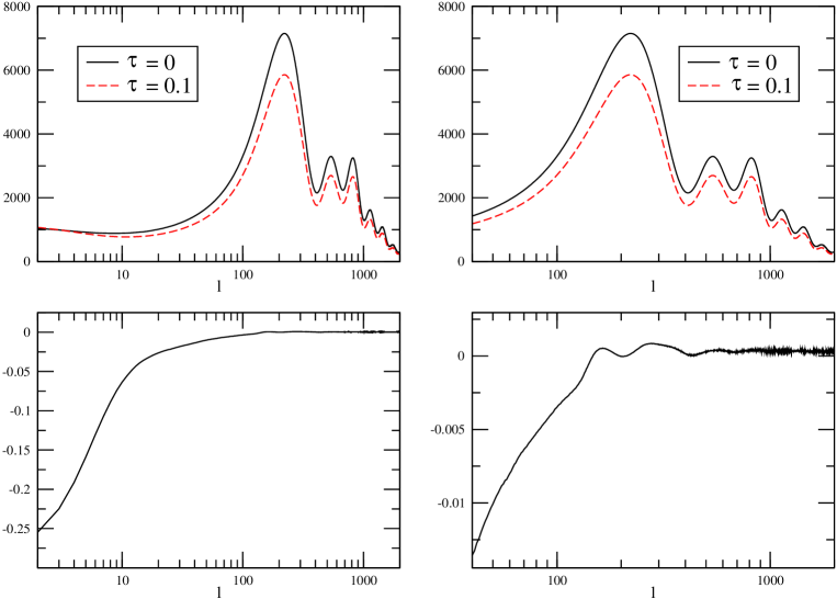
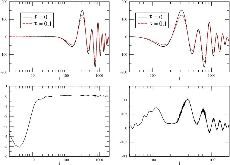
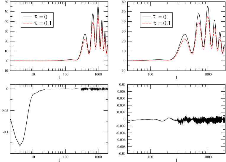
In this appendix we study the effect of reionization on the angular power spectrum of the CMB. If the baryons are reionized at redshift $z_{\mathrm{ri}}$, the effect on scales which are of the order of the horizon size at the time is complicated, and leads to additional polarization and a scale-dependent reduction of the amplitude of anisotropies. However, on scales which are well inside the horizon, the rescattering of photons simply reduces the amplitude of CMB temperature and polarization anisotropies by roughly the same amount on all scales. This effect can therefore be absorbed in a renormalization of the spectrum. In figure 9 we show the TT spectrum with and without reionization for the best-fit $\Lambda$CDM model, as well as the relative difference of the spectrum with and without reionization. For $\ell\geq 40$, renormalizing the spectrum with a constant reproduces the effect of reionization within about 1.5%. We have done the same with the temperature–polarization cross-correlation and the polarization spectra. Also there renormalization is a very good approximation (better than 0.5% on average) for $\ell\geq 40$, see figures 10 and 11. To obtain the spectra with $\tau=0.1$, we have multiplied the spectra with $\tau=0$ by the factor $0.82$.

Figure 9: The TT power spectrum with (dashed, red) and without (solid, black) reionization for optical depth $\tau=0.1$ for $\ell\geq 2$ (left upper panel) and $\ell\geq 40$ (right upper panel). For the upper panels, the vertical axis is $\ell(\ell+1)C^{TT}/(2\pi)$ in $(\mu K)^{2}$. In the lower panel we show the relative difference between the spectrum with and without reionization, when the latter is simply rescaled by a constant. For low $\ell$’s, the differences are substantial, up to 25%, but for the values $\ell\geq 40$ we consider, the difference is less than 2%.

Figure 10: The TE correlation spectrum with (dashed, red) and without (solid, black) reionization for optical depth $\tau=0.1$ for $\ell\geq 2$ (left upper panel) and $\ell\geq 40$ (right upper panel). The vertical axis is $\ell(\ell+1)C^{TT}/(2\pi)$ in $(\mu K)^{2}$. In the lower panel we show the difference between the spectrum with and without reionization, when the latter is simply rescaled by a constant. For the values $\ell\geq 40$ we consider, the difference is below $0.1(\mu K)^{2}$.

Figure 11: As in figure 10, but for the EE power spectrum. For $\ell\geq 40$, the difference is below $0.002(\mu K)^{2}$.

References

- [1]
- [2] E.V. Linder, The dynamics of quintessence, the quintessence of dynamics, Gen. Rel. Grav. 40 (2008) 339 [arXiv:0704.2064 [astro-ph]]
- [3] Salvatore Capozziello and Mauro Francaviglia, Extended theories of gravity and their cosmological and astrophysical applications, Gen. Rel. Grav. 40 (2008) 357 [arXiv:0706.1146 [astro-ph]]
- [4] K. Koyama The cosmological constant and dark energy in braneworlds, Gen. Rel. Grav. 40 (2008) 421 [arXiv:0706.1557 [astro-ph]]
- [5] R. Durrer and R. Maartens, Dark energy and dark gravity: theory overview, Gen. Rel. Grav. 40 (2008) 301 [arXiv:0711.0077 [astro-ph]]
- [6] S. Räsänen, Accelerated expansion from structure formation, JCAP11(2006)003 [arXiv:astro-ph/0607626]
- [7] T. Buchert, Dark Energy from Structure - A Status Report, Gen. Rel. Grav. 40 (2008) 467 [arXiv:0707.2153 [gr-qc]]
- [8] K. Enqvist, Lemaitre-Tolman-Bondi model and accelerating expansion, Gen. Rel. Grav. 40 (2008) 451 [arXiv:0709.2044] [astro-ph]
- [9] S. Räsänen, Evaluating backreaction with the peak model of structure formation, JCAP04(2008)026 [arXiv:0801.2692 [astro-ph]]
- [10] J.P. Zibin, A. Moss and D. Scott, Can we avoid dark energy?, Phys. Rev. Lett. 101 (2008) 251303 [arXiv:0809.3761 [astro-ph]]
- [11] M.N. Celerier, K. Bolejko, A. Krasinski and C. Hellaby, A (giant) void is not mandatory to explain away dark energy with a Lemaitre-Tolman model [arXiv:0906.0905 [astro-ph.CO]]
- [12] E. Komatsu et al.[WMAP Collaboration], Five-Year Wilkinson Microwave Anisotropy Probe (WMAP) Observations: Cosmological Interpretation, Astrophys. J. Suppl. 180 (2009) 330 [arXiv:0803.0547 [astro-ph]]
- [13] J. Dunkley et al. [WMAP Collaboration], Five-Year Wilkinson Microwave Anisotropy Probe (WMAP) Observations: Likelihoods and Parameters from the WMAP data, Astrophys. J. Suppl. 180 (2009) 306 [arXiv:0803.0586 [astro-ph]]
- [14] G. Hinshaw et al., Five-Year Wilkinson Microwave Anisotropy Probe (WMAP) Observations: Data Processing, Sky Maps, & Basic Results, Astrophys. J. Suppl. 180 (2009) 225 [arXiv:0803.0732 [astro-ph]]
- [15] C.L. Reichardt et al., High Resolution CMB Power Spectrum from the Complete ACBAR Data Set, Astrophys. J. 694 (2009) 1200 [arXiv:0801.1491v3 [astro-ph]]
- [16] G. Efstathiou and J.R. Bond, Cosmic Confusion: Degeneracies among Cosmological Parameters Derived from Measurements of Microwave Background Anisotropies, Mon. Not. Roy. Astron. Soc. 304 (1999) 75 [arXiv:astro-ph/9807103]
- [17] A. Kosowsky, M. Milosavlijevic and R. Jimenez, Efficent cosmological parameter estimation from microwave background anisotropies, Phys. Rev. D66 (2002) 063007 [arXiv:astro-ph/0206014]
- [18] Ø. Elgarøy and T. Multamäki, On using the CMB shift parameter in tests of models of dark energy, Astron. & Astrophys. 471 (2007) 65 [arXiv:astro-ph/0702343]
- [19] Y. Wang Y and P. Mukherjee, Observational Constraints on Dark Energy and Cosmic Curvature, Phys. Rev. D76 (2007) 103533 [arXiv:astro-ph/0703780]
- [20] P.S. Corasaniti and A. Melchiorri, Testing Cosmology with Cosmic Sound Waves, Phys. Rev. D77 (2008) 103507 [arXiv:0711.4119 [astro-ph]]
- [21] P. Mukherjee, M. Kunz, D. Parkinson and Y. Wang, Planck priors for dark energy surveys, Phys. Rev. D78 (2008) 083529 [arXiv:0803.1616 [astro-ph]]
- [22] E. Komatsu et al., Seven-Year Wilkinson Microwave Anisotropy Probe (WMAP) Observations: Cosmological Interpretation [arXiv:1001.4538 [astro-ph.CO]]
- [23] T. Clifton, P.G. Ferreira and J. Zuntz, What the small angle CMB really tells us about the curvature of the Universe, JCAP07(2009)029 [arXiv:0902.1313 [astro-ph.CO]]
- [24] S. Räsänen, On the relation between the isotropy of the CMB and the geometry of the universe, Phys. Rev. D79 (2009) 123522 [arXiv:0903.3013 [astro-ph.CO]]
- [25] U. Seljak, Rees-Sciama effect in a CDM Universe, Astrophys. J. 460 (1996) 549
- [26] A. Lewis and A. Challinor, Weak Gravitational Lensing of the CMB, Phys. Rept. 429 (2006) 1
- [27] R. Durrer, The Cosmic Microwave Background, 2008 Cambridge University Press, Cambridge
-
[28]
A. Lewis, A. Challinor and A. Lasenby,
Efficient computation of CMB anisotropies in closed FRW Models,
Astrophys. J. 538 (2000) 473
[arXiv:astro-ph/9911177]
A. Lewis and S. Bridle, Cosmological parameters from CMB and other data: a Monte Carlo approach, Phys. Rev. D66 (2002) 103511 [arXiv:astro-ph/0205436] (for updated versions see http://www.camb.info/) -
[29]
F.K. Hansen, A.J. Banday and K.M. Górski,
Testing the cosmological principle of isotropy: local power spectrum estimates of the WMAP data,
Mon. Not. Roy. Astron. Soc. 354 (2004) 641
[arXiv:astro-ph/0404206]
D. Huterer, Mysteries on Universe’s Largest Observable Scales, New Astron. Rev. 50 (2006) 868 [arXiv:astro-ph/0608318]
C.J. Copi, D. Huterer, D.J. Schwarz and G.D. Starkman, No large-angle correlations on the non-Galactic microwave sky, Mon. Not. Roy. Astron. Soc. 399 (2009) 399 [arXiv:0808.3767 [astro-ph]]
J. Hoftuft, H.K. Eriksen, A.J. Banday, K.M. Gorski, F.K. Hansen and P.B. Lilje, Increasing evidence for hemispherical power asymmetry in the five-year WMAP data, Astrophys. J. 699 (2009) 985 [arXiv:0903.1229 [astro-ph.CO]] - [30] F.K. Hansen, A.J. Banday, K.M. Gorski, H.K. Eriksen and P.B. Lilje, Power Asymmetry in Cosmic Microwave Background Fluctuations from Full Sky to Sub-degree Scales: Is the Universe Isotropic?, Astrophys. J. 704 (2009) 1448 [arXiv:0812.3795 [astro-ph]]
- [31] C.L. Francis and J.A. Peacock, An estimate of the local ISW signal, and its impact on CMB anomalies, [arXiv:0909.2495 [astro-ph.CO]]
- [32] C.L. Bennett et al., Seven-Year Wilkinson Microwave Anisotropy Probe (WMAP) Observations: Are There Cosmic Microwave Background Anomalies?, [arXiv:1001.4758 [astro-ph.CO]]
[33]
R.R. Caldwell, M. Doran, C.M. Mueller, G. Schafer and C. Wetterich,
Early quintessence in light of WMAP,
Astrophys. J. 591 (2003) L75
[arXiv:astro-ph/0302505]
E.V. Linder and G. Robbers, Shifting the Universe: Early Dark Energy and Standard Rulers, JCAP06(2008)004 [arXiv:0803.2877 [astro-ph]] -
[34]
S. Galli, F. Iocco, G. Bertone and A. Melchiorri,
CMB constraints on Dark Matter models with large annihilation cross-section,
Phys. Rev. D80 (2009) 023505
[arXiv:0905.0003 [astro-ph.CO]]
F. Iocco, Self-annihilating dark matter and the CMB: reionizing the Universe and constraining cross sections [arXiv:0912.1630 [astro-ph.CO]] -
[35]
N.P. Humphreys, R. Maartens and D.R. Matravers,
Anisotropic Observations in Universes with Nonlinear Inhomogeneity,
Astrophys. J. 477 (1997) 47
[arXiv:astro-ph/9602033]
H. Alnes and M. Amarzguioui, CMB anisotropies seen by an off-center observer in a spherically symmetric inhomogeneous universe, Phys. Rev. D74 (2006) 103520 [arXiv:astro-ph/0607334] -
[36]
C. Clarkson,
A covariant approach for perturbations of rotationally symmetric spacetimes,
Phys. Rev. D76 (2007) 104034
[arXiv:0708.1398 [gr-qc]]
J. P. Zibin, Scalar Perturbations on Lemaître-Tolman-Bondi Spacetimes, Phys. Rev. D78 (2008) 043504 [arXiv:0804.1787 [astro-ph]]
C. Clarkson, T. Clifton and S. February, Perturbation Theory in Lemaitre-Tolman-Bondi Cosmology, JCAP06(2009)025 [arXiv:0903.5040 [astro-ph.CO]] -
[37]
V. Mukhanov,
CMB-slow, or How to Estimate Cosmological Parameters by Hand,
Int. J. Theor. Phys. 43 (2004) 623
[astro-ph/0303072]
V. Mukhanov, Physical Foundations of Cosmology, 2005 Cambridge University Press, Cambridge - [38] S. Räsänen, Light propagation in statistically homogeneous and isotropic dust universes, JCAP02(2009)011 [arXiv:0812.2872 [astro-ph]]
[39]
A.G. Doroshkevich and M.Y. Khlopov,
On The Physical Nature Of Hidden Mass In The Universe,
Sov. J. Nucl. Phys. 39 (1984) 551 (Yad. Fiz. 39 (1984) 869)
M.S. Turner, G. Steigman and L.M. Krauss, The Flatness Of The Universe: Reconciling Theoretical Prejudices With Observational Data, Phys. Rev. Lett. 52 (1984) 2090
F. Ferrer, C. Nipoti and S. Ettori, Secular evolution of galaxies and galaxy clusters in decaying dark matter cosmology, Phys. Rev. D80 (2009) 061303 [arXiv:0905.3161 [astro-ph.CO]] -
[40]
L. Kofman, D. Pogosyan and A.A. Starobinsky,
The large scale microwave backbround anisotropy in unstable cosmologies,
Sov. Astron. Lett. 12 (1986) 175 (Pisma Astron. Zh. 12 (1986) 419)
K. Ichiki, M. Oguri and K. Takahashi, WMAP Constraints on Decaying Cold Dark Matter, Phys. Rev. Lett. 93 (2004) 071302 [arXiv:astro-ph/0403164]
S. De Lope Amigo, W.Y. Cheung, Z. Huang and S.P. Ng, Cosmological Constraints on Decaying Dark Matter, JCAP06(2009)005 [arXiv:0812.4016 [hep-ph]] - [41] W. Hu and N. Sugiyama, Small scale cosmological perturbations: An Analytic approach, Astrophys. J. 471 (1996) 542 [arXiv:astro-ph/9510117]
- [42] Spergel D N et al.[WMAP Collaboration], Wilkinson Microwave Anisotropy Probe (WMAP) three year results: Implications for cosmology, Astrophys. J. Suppl. 170 (2007) 377 [arXiv:astro-ph/0603449]
[43]
C. Clarkson, B.A. Bassett and T. H.-C. Lu,
A general test of the Copernican Principle,
Phys. Rev. Lett. 101 (2008) 011301
[arXiv:0712.3457]
C. Clarkson, M. Cortes, B.A. Bassett, Dynamical Dark Energy or Simply Cosmic Curvature?, JCAP0708(2007)011. [arXiv:astro-ph/0702670]
A. Shafieloo and C. Clarkson Model independent tests of the standard cosmological model [arXiv:0911.4858] -
[44]
R. Jimenez and A. Loeb,
Constraining Cosmological Parameters Based on Relative Galaxy Ages,
Astrophys. J. 573 (2002) 37
[arXiv:astro-ph/0106145]
J. Simon, L. Verde and R. Jimenez, Constraints on the redshift dependence of the dark energy potential, Phys. Rev. D71 (2005) 123001 [arXiv:astro-ph/0412269] -
[45]
E. Gaztañaga, A. Cabré and L. Hui,
Clustering of Luminous Red Galaxies IV: Baryon Acoustic Peak in the Line-of-Sight Direction and a Direct Measurement of H(z),
Mon. Not. Roy. Astron. Soc. 399 (2009) 1663
[arXiv:0807.3551 [astro-ph]]
E. Gaztañaga, R. Miquel and E. Sánchez, First Cosmological Constraints on Dark Energy from the Radial Baryon Acoustic Scale, Phys. Rev. Lett. 103 (2009) 091302 [arXiv:0808.1921 [astro-ph]] - [46] W. Hu, M. Fukugita, M. Zaldarriaga and M. Tegmark, CMB Observables and Their Cosmological Implications, Astrophys. J. 549 (2001) 669 [arXiv:astro-ph/0006436]
- [47] M. Doran and M. Lilley, The Location of CMB Peaks in a Universe with Dark Energy, Mon. Not. Roy. Astron. Soc. 330 (2002) 965 [arXiv:astro-ph/0104486]
- [48] L.M. Krauss and B. Chaboyer, Age Estimates of Globular Clusters in the Milky Way: Constraints on Cosmology, Science 299 (2003) 65
- [49] J. P. Zibin, A. Moss and D. Scott, The Evolution of the Cosmic Microwave Background, Phys. Rev. D76 (2007) 123010 [arXiv:0706.4482v3 [astro-ph]]
- [50] A.E. Raftery and S.M. Lewis How many iterations in the Gibbs sampler?, 1992 Bayesian Statistics 4, pp. 763-773 Cambridge University Press, Cambridge
- [51] H. Kurki-Suonio, V. Muhonen and J. Väliviita, Correlated Primordial Perturbations in Light of CMB and LSS Data, Phys. Rev. D71 (2005) 063005 [arXiv:astro-ph/0412439]
[52]
R.H. Becker et al.,
Evidence for Reionization at : Detection of a
Gunn-Peterson Trough in a z=6.28 Quasar,
Astron. J. 22 (2001) 2850
[arXiv:astro-ph/0108097]
X. Fan et al., Observational constraints on Cosmic Reionization, Ann. Rev. Astron. Astrophys. 44 (2006) 415 [arXiv:astro-ph/0602375] - [53] C. Amsler et al. [Particle Data Group], Review of particle physics, Phys. Lett. B667 (2008) 1
- [54] P. Gondolo et al., DarkSUSY: Computing Supersymmetric Dark Matter Properties Numerically, JCAP07(2004)008 [arXiv:astro-ph/0406204]