Branch and Bound Algorithms for Maximizing Expected Improvement Functions

Abstract

Deterministic computer simulations are often used as a replacement for complex physical experiments. Although less expensive than physical experimentation, computer codes can still be time-consuming to run. An effective strategy for exploring the response surface of the deterministic simulator is the use of an approximation to the computer code, such as a Gaussian process (GP) model, coupled with a sequential sampling strategy for choosing design points that can be used to build the GP model. The ultimate goal of such studies is often the estimation of specific features of interest of the simulator output, such as the maximum, minimum, or a level set (contour). Before approximating such features with the GP model, sufficient runs of the computer simulator must be completed.

Sequential designs with an expected improvement (EI) function can yield good estimates of the features with a minimal number of runs. The challenge is that the expected improvement function itself is often multimodal and difficult to maximize. We develop branch and bound algorithms for efficiently maximizing the EI function in specific problems, including the simultaneous estimation of a minimum and a maximum, and in the estimation of a contour. These branch and bound algorithms outperform other optimization strategies such as genetic algorithms, and over a number of sequential design steps can lead to dramatically superior accuracy in estimation of features of interest.

1 Introduction

Computer experiments are often employed to simulate complex systems, but realistic computer simulators of physical phenomena can be time consuming to evaluate. In such cases it is desirable to perform the experiment as efficiently as possible. One popular approach designed for this purpose is sequential experimental design (Jones, 2001) whereby an initial design is simulated and a surrogate model is fit to the output, often using a Gaussian Spatial Process (Sacks et al., 1989). The surrogate provides estimates at all input combinations (sampled and unsampled) with accompanying variance estimates and is used, along with a suitable ‘infill criterion’, to choose subsequent trials.

Scientists are often interested in specific features of the simulator, such as the maximum, the minimum, level set(s), etc. In each case, the follow-up trial in the sequential design is selected so as to give the greatest improvement to the estimate(s) of these feature(s) of interest. A popular approach is to choose this new trial by maximizing a merit-based infill criterion. Many criteria have been proposed (Jones et al., 1998) (Villemonteix et al., 2006) (Forrester and Jones, 2008) and one popular choice is the ‘expected improvement’. This criteria has been shown to be efficient if the initial design is not too sparse or deceptive (Forrester and Jones, 2008).

The form of the improvement function varies with the features of interest, but in any case facilitates a balance between choosing points that exhibit local optimality (greedy search, new trials close to predicted feature of interest), and points with high uncertainty (global search, new trials away from previously sampled points) (Papalambros et al., 2002). Finding the next design point (the point that maximizes the EI function) is necessary in order to ensure the estimation of features of interest in the smallest number of simulator runs. Finding this maximum is a difficult global optimization problem, and the addition of each point in the sequential design changes the EI function, requiring another search for the global optimum of EI in order to find the next point.

The main focus of this paper is to develop branch and bound algorithms for maximizing expected improvement functions for two particular features of interest; contours, and the simultaneous estimation of maximum and minimum. The most challenging aspect of this algorithm is constructing the bounds on the objective function (expected improvement). Branch and bound algorithms have been implemented for finding the minimum of a function (Jones et al., 1998), and expected improvement criteria have been developed for the minimum (Jones et al., 1998), and contours (Ranjan et al., 2008). Our main contribution are in (a) generalizing the expected improvement criterion for simultaneous estimation of the maximum and minimum, and (b) developing branch and bound algorithms for maximizing expected improvement for contours, and for simultaneous maximum/minimum estimation. Ranjan et al. (2008) maximized their expected improvement function for estimating contours using a genetic algorithm. The branch and bound algorithm developed here outperforms their optimization by locating level sets using fewer simulator runs.

This paper is organized as follows: Section 2 gives an overview of the Gaussian process model, the expected improvement criterion and a generic branch and bound algorithm which will be used to maximize the expected improvement over candidate input points. In Section 3 we propose bounds on the expected improvement for estimating contours and simultaneous estimation of the global maximum and minimum. Section 4 presents simulation results comparing our branch and bound and a genetic algorithm similar to that of Ranjan et al. (2008) for different test functions. We present our conclusions and outline possible future work in Section 5.

2 Review - surrogate model, global optimization

2.1 Gaussian Process Model

Let $y_{i}$ represent the univariate response from the computer simulator, and $\mathbf{X}=(\mathbf{x}_{1},\mathbf{x}_{2},...,\mathbf{x}_{n})^{\prime}$ be the matrix of input vectors $\mathbf{x}_{i}^{\prime}=(x_{i1},x_{i2},...,x_{id})$ used to generate the respective outputs, with $y(\mathbf{X})=(y_{1},y_{2},...,y_{n})^{\prime}$. Without loss of generality, let the input space be the unit hypercube $\chi=[0,1]^{d}$. Following Sacks et al. (1989) we model the output $y(\mathbf{x}_{i})$ as

$$y(\mathbf{x}_{i})=\mu+z(\mathbf{x}_{i});\qquad i=1,...,n,$$ (1)

where $\mu$ is the overall mean, and $\{z(\mathbf{x}),x\in\chi\}$ is a Gaussian spatial process with mean 0, variance $\sigma^{2}_{z}$ and corr$(z(\mathbf{x}_{i}),z(\mathbf{x}_{j}))=R_{ij}$. The correlation matrix $R$ is a function of the hyper-parameters $\bm{\theta}=(\theta_{1},\ldots,\theta_{d})$. In general, $y(X)$ has multivariate normal distribution, $y(X)\sim N_{n}({\bf 1_{n}}\mu,\sigma^{2}_{z}R)$, where the parameters $\Omega=(\theta_{1},...,\theta_{d};\mu,\sigma^{2}_{z})$ are estimated by maximizing the likelihood. The mean and variance parameters have closed form estimates given by

$$\hat{\mu}=(\bm{1_{n}}^{\prime}R^{-1}\bm{1_{n}})^{-1}\bm{1_{n}}^{\prime}R^{-1}\bm{y}\quad\mathrm{and}\quad\hat{\sigma}^{2}_{z}=\frac{(\bm{y}-\bm{1_{n}}\hat{\mu})^{\prime}R^{-}1(\bm{y}-\bm{1_{n}}\hat{\mu})}{n},$$ (2)

whereas the hyper-parameters $\bm{\theta}=(\theta_{1},...,\theta_{d})$ are estimated by maximizing the profile likelihood.

The best linear unbiased predictor (BLUP) at $x^{*}$, $\hat{y}(x^{*})$, and the associated mean squared error (MSE) $s^{2}(x^{*})$ are given by

$$\hat{y}(x^{*})=\ \hat{\mu}+r^{\prime}R^{-1}(y-\mathbf{1}_{n}\hat{\mu}),$$ (3)

$$s^{2}(y(x^{*}))=\ \sigma_{z}^{2}\left(1-r^{\prime}R^{-1}r+\frac{(1-\mathbf{1}^{\prime}_{n}R^{-1}r)^{2}}{\mathbf{1}^{\prime}_{n}R^{-1}\mathbf{1}_{n}}\right),$$ (4)

where $r=(r_{1}(x^{*}),...,r_{n}(x^{*}))^{\prime}$ and $r_{i}(x^{*})=\mathrm{corr}(z(x^{*}),z(x_{i}))$. The estimates $\hat{y}(x^{*})$ and $\hat{s}(x^{*})$ are obtained by replacing $R$, $r$ and $\sigma^{2}_{z}$ with $\hat{R}(\bm{\hat{\theta}})$, $\hat{r}(\bm{\hat{\theta}})$ and $\hat{\sigma}^{2}_{z}$. There are innumerable choices for the correlation structure, for instance, power exponential correlation and Matérn correlation (see Stein (1999); Santner et al. (2003) for details). The choice of correlation function is not crucial to the algorithms and methodologies developed here, and thus we omit the details. In all illustrations, the power exponential correlation function is used.

It turns out that if the design points are close together in the input space the correlation matrix $R$ can sometimes be near-singular which results in unstable computation. A popular approach to overcome this problem is to introduce a small nugget $0<\delta<1$ and approximate the ill-conditioned $R^{-1}$ with a well-conditioned $(R+\delta I)^{-1}$, where $I$ is the $n\times n$ identity matrix. In later sections, a nugget is included in the GP model.

2.2 Sequential design using EI criterion

For expensive computer models the total number of simulator runs is limited; and thus the choice of design points is crucial for estimating certain pre-specified features or approximating the underlying process. If we are interested in only certain features (e.g., global maxima, contours, and so on) of the process, a popular approach is to use a sequential sampling strategy. The key steps of such a sampling strategy are summarized as follows:

1. Choose an initial design $\{x_{1},...,x_{n_{0}}\}$.

2. Run the simulator, $f$, for these design settings to get $\{y_{1},...,y_{n_{0}}\}$, where $y_{i}=f(x_{i})$. Set $n=n_{0}$.

3. Fit a surrogate to the data $\{(x_{i},y_{i}),i=1,...,n\}$ (we use the Gaussian process model).

4. Choose a new trial $x_{new}$ that leads to improvement in the estimate of the feature of interest.

5. Run the simulator for the new trial location and update the data $x_{n+1}=x_{new}$, $y_{n+1}=f(x_{new})$ and $n=n+1$.

6. Repeat 3-5 until $n$ exceeds a predetermined limit.

Developing feature specific criteria for selecting new trials has gained considerable attention in the computer experiment community. For instance, Jones et al. (1998) proposed an expected improvement (EI) criterion for estimating the global minimum of an expensive computer simulator. Let $I(x)$ denote the improvement function for estimating a particular feature of interest. Then, the proposed criterion in Jones et al. (1998) is $E[I_{1}(x)]$, where $I_{1}(x)=\max\{f_{min}-y(x),0\}$, $f_{min}$ is the current best estimate of the function minimum, and the expectation is taken over the distribution of $y(x)\sim N(\hat{y}(x),s^{2}(x))$. That is, the new trial in Step 4 is the maximizer of

$$E[I_{1}(x)]=s(x)\phi(u)+(f_{min}-\hat{y}(x))\Phi(u),$$ (5)

where $u=(f_{min}-\hat{y}(x))/s(x)$, and $\phi(\cdot)$ and $\Phi(\cdot)$ denote standard normal pdf and cdf respectively. One of the most attractive characteristics of the EI criterion is that it exhibits a balance between ‘global’ and ‘local’ search. The first term in $(\ref{ei_min})$ supports global search, and the second term, local search.

Since the main objective of performing a good design is to attain (or at least reach a good approximation of) the global minimum in as few simulator runs as possible, efficient optimization of the EI function becomes very important. The EI functions are often multimodal and the location, number and heights of these peaks change after adding every new trial. Jones et al. (1998) developed a branch and bound (BNB) algorithm for optimizing the EI function (5), which we review briefly in the next section.

2.3 Branch and bound algorithm: review for finding a global minimum

BNB algorithms are often used for global optimization of non-convex functions (Lawler and Wood, 1966; Moore, 1991). The BNB algorithm presented here finds the global minimum of a real-valued function $g$. In our case, $g(x)=-E[I(x)]$ is defined on the $d$-dimensional hypercube $\mathcal{Q}_{init}=\chi=[0,1]^{d}$ for a specific feature of interest.

There are three key components of a BNB algorithm - (i) branching (ii) bounding and (iii) pruning. The branching component uses a splitting procedure that, given a rectangle $\mathcal{Q}\subset\mathcal{Q}_{init}$, returns $\mathcal{Q}_{I}$ and $\mathcal{Q}_{II}$ such that $\mathcal{Q}_{I}\cap\mathcal{Q}_{II}=\phi$ (null) and $\mathcal{Q}_{I}\cup\mathcal{Q}_{II}=\mathcal{Q}$. The splitting occurs along the longest edge of $\mathcal{Q}$ (if there is a tie, one is chosen randomly). Bounding is the second component. Bounding the objective function $g$, requires finding the lower and upper bounds, $\Psi_{lb}$ and $\Psi_{ub}$, of the minimum value of $g$. Let $\Psi_{min}(\mathcal{Q})=\min_{x\in\mathcal{Q}}g(x)$ for every $\mathcal{Q}\subset\mathcal{Q}_{init}$, then $\Psi_{lb}$ and $\Psi_{ub}$ must satisfy

$$R1\quad : \Psi_{lb}(\mathcal{Q})\leq\Psi_{min}(\mathcal{Q})\leq\Psi_{ub}(\mathcal{Q})$$

$$R2\quad : \forall\;\epsilon>0\;\exists\;\delta>0\;\textrm{such that for all}\;\mathcal{Q}\subseteq\mathcal{Q}_{init},$$

$$|\mathcal{Q}|\leq\delta\;\Longrightarrow\;\Psi_{ub}(\mathcal{Q})-\Psi_{lb}(\mathcal{Q})\leq\epsilon.$$

As in Balakrishnan et al. (1991), $|\mathcal{Q}|$ is the length of the longest edge of rectangle $\mathcal{Q}$. Although BNB algorithms guarantee the global minimum of $g$ with a pre-specified tolerance $\epsilon$, the bounding functions $\Psi_{lb}$ and $\Psi_{ub}$ are objective function specific and often nontrivial to derive. This is the most challenging part of a BNB algorithm. Appropriate lower and upper bounds can be constructed for maximizing the EI criteria for a few specific process features of interest, and this is the main contribution of the paper. The third component of the BNB algorithm is pruning, in which the algorithm removes rectangles $\mathcal{Q}$ from the set of all rectangles $\mathfrak{L}$, that have lower bound greater than the upper bound of some other rectangle in $\mathfrak{L}$. In the BNB algorithm outlined below, individual rectangles are represented by $\mathcal{Q}$’s and lists of rectangles are represented by $\mathfrak{L}$’s:

1 $k=0$                        (initialize counter)
2 $\mathfrak{L}_{0}=\{\mathcal{Q}_{init}\}$                        (initialize rectangle list)
3 $L_{0}=\Psi_{lb}\{\mathcal{Q}_{init}\}$
4 $U_{0}=\Psi_{ub}\{\mathcal{Q}_{init}\}$
5 while $U_{k}-L_{k}>\epsilon$
6      $Pick\;\mathcal{Q}\in\mathfrak{L}_{k}\;:\;\Psi_{lb}(\mathcal{Q})=L_{k}$
7      $Split\;\mathcal{Q}\;along\;one\;of\;its\;longest\;edges\;into\;\mathcal{Q}_{I}\;and\mathcal{Q}_{II}$
8      $\mathfrak{L}_{k+1}:=(\mathfrak{L}_{k}\backslash\{\mathcal{Q}\})\cup\{\mathcal{Q}_{I},\mathcal{Q}_{II}\}$             (remove $\mathcal{Q}$, replace with
                                                                             $\mathcal{Q}_{I}$ and $\mathcal{Q}_{II}$ to get $\mathfrak{L}_{k+1}$)
9      $L_{k+1}:=min_{\mathcal{Q}\in\mathfrak{L}_{k+1}}\Psi_{lb}(\mathcal{Q})$
10    $U_{k+1}:=min_{\mathcal{Q}\in\mathfrak{L}_{k+1}}\Psi_{ub}(\mathcal{Q})$
11    $\mathfrak{L}_{k+1}:=\mathfrak{L}_{k+1}\setminus\{\mathcal{Q}\in\mathfrak{L}_{k+1}:\Psi_{lb}(\mathcal{Q})>U_{k+1}\}$
12    $k=k+1$
13 $end$

In this algorithm, $k$ is the iteration index, $\mathfrak{L}_{k+1}$ is the list of hyper-rectangles, $(L_{k+1},U_{k+1})$ are the smallest lower and upper bounds for $\Psi_{min}(\mathcal{Q}_{init})$ (in our case $\min_{x\in\chi}-E[I(x)]$) after $k+1$ iterations, and $\epsilon$ is the desired precision and is fixed beforehand. Steps 6-8 correspond to branching, Steps 9-10 bounding, and Step 11 represents pruning of the hyper-rectangles.

The EI function, $E[I_{1}(x)]$, for finding the global minimum of the simulator, is a function of the input location $x$ via the predicted response $\hat{y}(x)$, the associated uncertainty $s^{2}(x)$ at $x$ and the current estimate of the global minimum $f_{min}$ (in general the estimate of the feature of interest). Jones et al. (1998) note that $E[I_{1}(x)]$ is monotonic with respect to (w.r.t.) $\hat{y}(x)$ and $s(x)$. Let $EI_{1}(s(x),\hat{y}(x))$ denote $E[I_{1}(x)]$ for all $x\in\chi$. Taking partial derivatives of $(\ref{ei_min})$ w.r.t. $\hat{y}(x)$ and $s(x)$ give

$$\frac{\partial EI_{1}}{\partial s(x)}=\phi\left(u\right)\quad\textrm{and}\quad\frac{\partial EI_{1}}{\partial\hat{y}(x)}=-\Phi\left(u\right).$$

The partial derivatives $\partial EI_{1}/\partial s(x)\geq 0$ and $\partial EI_{1}/\partial\hat{y}(x)\leq 0$ for all $x\in\chi$. Hence if $\hat{y}(x)$ and $s(x)$ can be bounded by $(\hat{y}_{lb}(\mathcal{Q}),\hat{y}_{ub}(\mathcal{Q}))$ and $(s_{lb}(\mathcal{Q}),s_{ub}(\mathcal{Q}))$ respectively over a hyper-rectangle $\mathcal{Q}\in\mathfrak{L}$, then for every $x\in\mathcal{Q}$, the lower and upper bounds $E[I_{1}(x)]_{ub}=\Psi_{lb}(\mathcal{Q})$ and $E[I_{1}(x)]_{lb}=\Psi_{ub}(\mathcal{Q})$ are

$$E[I_{1}(x)]_{lb} =EI_{1}(s_{lb}(\mathcal{Q}),\hat{y}_{ub}(\mathcal{Q})),$$

$$E[I_{1}(x)]_{ub} =EI_{1}(s_{ub}(\mathcal{Q}),\hat{y}_{lb}(\mathcal{Q})),$$

where $\hat{y}_{lb}(\mathcal{Q}),\hat{y}_{ub}(\mathcal{Q}),s_{lb}(\mathcal{Q})$ and $s_{ub}(\mathcal{Q})$ are the lower and upper bounds on $\hat{y}(x)$ and $s(x)$ over $\mathcal{Q}$. These bounds are needed in Steps 6-11. In practice $s(x)$ is replaced by its predicted value $\hat{s}(x)$. This approach of bounding the EI function is efficient, as bounding $s(x)$ and $\hat{y(x)}$ is relatively easier (see Jones et al. (1998) for details).

3 BNB Algorithms for New EI Criteria

In this section we first propose a generalization of the expected improvement criterion developed by Jones et al. (1998) for simultaneously estimating the maximum and minimum of an expensive deterministic computer simulator. Next we develop a BNB algorithm for maximizing this new EI criterion. We also propose a modification in the EI criterion developed by Ranjan et al. (2008) for estimating a pre-specified contour. This modification facilitates the development of a BNB algorithm for maximizing the modified EI criterion, and still maintains the global versus local search trade-off.

3.1 EI criterion for maximum and minimum

We propose an improvement function for simultaneous estimation of the global maximum and minimum. This feature could be of specific interest, for instance, if one wishes to identify best-case and worst-case scenarios in a global climate change model, or maximal and minimal projected unemployment rates in a complex model of the economy. The improvement function can be written as

$$I_{2}(x)=\max\{(y(\mathbf{x})-f_{max}),(f_{min}-y(\mathbf{x})),0\},$$ (7)

where $f_{max}$ and $f_{min}$ are current best estimates of the global maximum and minimum respectively. The corresponding expected improvement criterion is obtained by taking the expectation of $I_{2}(x)$ with respect to the distribution of $y(x)\sim N(\hat{y}(x),s^{2}(x))$,

$$E[I_{2}(x)]=s\phi(u_{1})+(\hat{y}-f_{max})\Phi(u_{1})+s\phi(u_{2})+(f_{min}-\hat{y})\Phi(u_{2}),$$ (8)

where $u_{1}=(\hat{y}-f_{max})/s$ and $u_{2}=(f_{min}-\hat{y})/s$. The EI criterion (8) turns out to be the sum of the two EI criteria for individually estimating the global maximum and the global minimum. Optimization of (8) favors subsequent sampling in the neighbourhood of the global maximum if $(\hat{y}-f_{max})\Phi(u_{1})$ is the dominating term in the sum, the global minimum if $(f_{min}-\hat{y})\Phi(u_{2})$ is the dominant term, and otherwise in the less explored regions to minimize overall variability.

As in optimization of the EI criterion (5) for estimating the global minimum, a BNB algorithm can be developed for optimizing (8). The most difficult part, computation of the lower and upper bounds of (8) that satisfy $R1$ and $R2$ in (2.3) for minimizing $g(x)=-E[I_{2}(x)]$, is accomplished by monotonicity of the $E[I_{2}(x)]$ w.r.t. $\hat{y}(x)$ and $s(x)$. Let $EI_{2}(s(x),\hat{y}(x))$ denote $E[I_{2}(x)]$ for all $x\in\chi$. Then the two partial derivatives of $E[I_{2}(x)]$ are

$$\frac{\partial EI_{2}}{\partial s(\mathbf{x})}=\phi\left(u_{1}\right)+\phi\left(u_{2}\right)\quad\textrm{and}\quad\frac{\partial EI_{2}}{\partial\hat{y}(\mathbf{x})}=\Phi\left(u_{1}\right)-\Phi\left(u_{2}\right).$$

The partial derivative w.r.t. $s(x)$ is positive for all $x\in\chi$, and the partial derivative w.r.t. $\hat{y}(x)$ is equal to zero when $\hat{y}(\mathbf{x})=\frac{(f_{max}+f_{min})}{2}$. Moreover, it is straightforward to show that

$$\frac{\partial EI_{2}}{\partial\hat{y}(\mathbf{x})}\left\{\begin{array}[]{ll}\geq 0&\textrm{if}\ \hat{y}(\mathbf{x})>\frac{(f_{max}+f_{min})}{2}\\ \leq 0&\textrm{if}\ \hat{y}(\mathbf{x})<\frac{(f_{max}+f_{min})}{2}\\ \end{array}.\right.$$

Hence $E[I_{2}(x)]$ is monotonic for all $x\in\chi$ w.r.t. $s(x)$ and piecewise monotonic w.r.t. $\hat{y}(\mathbf{x})$. Given the upper and lower bounds on $\hat{y}(\mathbf{x})$ and $s(\mathbf{x})$ in a hyper-rectangle $\mathcal{Q}\subset\mathcal{Q}_{init}$, somewhat conservative bounds on $E[I_{2}(\bm{x})]$, for every $x\in\mathcal{Q}$, are

$$E[I_{2}(x)]_{lb}=\min\{ EI_{2}(s_{lb}(\mathcal{Q}),\hat{y}_{lb}(\mathcal{Q})),EI_{2}(s_{lb}(\mathcal{Q}),\hat{y}_{ub}(\mathcal{Q}))\},$$

$$E[I_{2}(x)]_{ub}=\max\{ EI_{2}(s_{ub}(\mathcal{Q}),\hat{y}_{lb}(\mathcal{Q})),EI_{2}(s_{ub}(\mathcal{Q}),\hat{y}_{ub}(\mathcal{Q}))\}.$$

That is, the upper bound of $E[I_{2}(x)]$ in $\mathcal{Q}$ is calculated at $s_{ub}(\mathcal{Q})$, and due to piecewise monotonicity of $E[I_{2}(x)]$, corresponds to the $\hat{y}(\mathbf{x})$ in $\mathcal{Q}$ that is closest to $f_{min}$ or $f_{max}$. Similarly, the lower bound of $E[I_{2}(x)]$ is calculated using $s_{lb}(\mathcal{Q})$ and the $\hat{y}(\mathbf{x})$ in $\mathcal{Q}$ that is closest to $(f_{max}+f_{min})/2$.

These bounds are conservative because the lower and upper bounds of $s(x)$ and minimizer of $|\hat{y}(x)-(f_{max}+f_{min})/2|$ may not correspond to the same point in the input space. The lower bound $\Psi_{lb}(\mathcal{Q})$ of $\min_{x\in\mathcal{Q}}(-E[I_{2}(x)])$ will be equal to the true minimum of $-E[I_{2}(x)]$ only if the minimizers of $s(x)$ and $|\hat{y}(x)-(f_{max}+f_{min})/2|$ are identical. As a result, the hyper-rectangles in $\mathfrak{L}$ are pruned at a slower rate.

3.2 BNB algorithm for contour estimation problem

The use of a EI criterion for estimating a contour (level set) of an expensive computer simulator was proposed by Ranjan et al. (2008). The motivating application involved distinguishing “good” from “bad” performance of a server in a one-server-two-queue network queuing simulator. The proposed improvement function for estimating the contour $S(a)=\{x:y(x)=a\}$ was $I_{3}(x)=\epsilon^{2}(x)-\min\{(y(x)-a)^{2},\epsilon^{2}(x)\}$, where $\epsilon(x)=\alpha s(x)$, for a positive constant $\alpha$, defines a neighbourhood around the contour. The expectation of $I(x)$ w.r.t. $y(x)\sim N(\hat{y}(x),s^{2}(x))$ is given by

$$E[I_{3}(x)]= \ \left[\epsilon^{2}(x)-(a-\hat{y}(x))^{2}\right]\left[\Phi\left(u_{1}\right)-\Phi\left(u_{2}\right)\right]$$ (9)

$$-2(a-\hat{y}(x))s(x)\left[\phi\left(u_{1}\right)-\phi\left(u_{2}\right)\right]-s^{2}(x)\int_{u_{1}}^{u_{2}}w^{2}\phi\left(w\right)dw,$$

where $u_{1}=(a-\hat{y}(x)+\epsilon(x))/s(x)$, $u_{2}=(a-\hat{y}(x)-\epsilon(x))/s(x)$, and $\phi(\cdot)$ and $\Phi(\cdot)$ are the standard normal pdf and cdf respectively. Ranjan et al. (2008) use $E[I_{3}(x)]$ as the EI criterion for selecting additional new trials in the sequential sampling strategy. However, controlling the trade-off between local and global search has gained attention in the area of computer experiments (e.g., Schonlau, Welch and Jones (1998), Sóbester, Leary, and Keane (2005)). This motivated us to modify the EI criterion in (9) that will facilitate the construction of the lower and upper bounds which satisfy $R1$ and $R2$ in (2.3), and still entertains the global versus local search trade-off.

Note that the third term in (9) represents the total uncertainty in the $\epsilon$-neighbourhood of the contour at $x$, and can be dropped without altering the important features of the criterion. We propose a modified EI criterion, obtained by dropping the third term in (9) and using a change of variable $\{\hat{y}(x),s(x)\}\rightarrow\{t(x),s(x)\}$, given by

$$E[I_{3}^{*}(x)]= \ s^{2}(x)\left[\alpha^{2}-t^{2}\right]\left[\Phi\left(t+\alpha\right)-\Phi\left(t-\alpha\right)\right]$$ (10)

$$-2ts^{2}(x)\left[\phi\left(t+\alpha\right)-\phi\left(t-\alpha\right)\right],$$

where $t=(a-\hat{y}(x))/s(x)$. Although the proposed modification slightly alters the tradeoff between the global and local search (see Section 4.1 for more details), it allows the partial derivatives of $E[I_{3}^{*}(x)]$ to be piecewise monotone. Furthermore, this facilitates easy construction of lower and upper bounds in the BNB algorithm for efficient optimization of $E[I_{3}^{*}(x)]$.

Let $EI_{3}^{*}(s(x),t(x))$ denote $E[I_{3}^{*}(x)]$ for all $x\in\chi$. Then, the partial derivative of $E[I_{3}^{*}(x)]$ w.r.t. $t=t(x)$ is

$$\frac{\partial EI_{3}^{*}}{\partial t} = -2s^{2}(x)t[\Phi(t+\alpha)-\Phi(t-\alpha)]+2\alpha s^{2}(x)t[\phi(t+\alpha)+\phi(t-\alpha)]$$ (11)

$$+\ s^{2}(x)(\alpha^{2}+t^{2}-2)[\phi(t+\alpha)-\phi(t-\alpha)].$$

It turns out that the sign of the partial derivative $\partial EI_{3}^{*}/\partial t$ depends on the sign of $t=(a-\hat{y}(x))/s(x)$. Since the normal pdf is symmetric around the mean (i.e., $\phi(u)=\phi(-u)$, for all $u$), the partial derivative $\partial EI_{3}^{*}/\partial t=0$ at $t=0$. In general,

$$\frac{\partial EI_{3}^{*}}{\partial t}\left\{\begin{array}[]{ll}\leq 0&\textrm{if}\ t>0\\ =0&\textrm{if}\ t=0\\ \geq 0&\textrm{if}\ t<0\\ \end{array}.\right.$$

Due to the presence of normal pdf and cdf in (11), it may not be straightforward to analytically prove the monotonicity result, however, it can easily be plotted (see Figure 1).

Figure 1: Partial derivative of $EI_{3}^{*}(t(x),s(x))$ w.r.t. $t(x)$ evaluated at $\alpha=2$.

There are a few points worth noting. For instance, the height of these peaks, in Figure 1, increases with $s$. The magnitude and sign of the derivative depend on the choice of $\alpha$ (we used $\alpha=2$). Interestingly, the nature of the curves remain the same for $\alpha>1$ (approximately).

The partial derivative $EI_{3}^{*}$ w.r.t. $s(x)$ is given by

$$\frac{\partial EI_{3}^{*}}{\partial s(x)} = 2s(x)(\alpha^{2}-t^{2})[\Phi(t+\alpha)-\Phi(t-\alpha)]$$ (12)

$$-4ts(x)[\phi(t+\alpha)-\phi(t-\alpha)].$$

The partial derivative $\partial EI_{3}^{*}/\partial s(x)$ is always non-negative. However, as with the monotonicity of $EI_{3}^{*}(s(x),t(x))$ with respect to $t(x)$, analytic proof may be somewhat complicated. Figure 2 displays the partial derivative $\partial EI_{3}^{*}/\partial s(x)$ as a function of $s(x)$.

As in the simultaneous estimation of the global maximum and minimum case, bounds on $E[I_{3}^{*}(x)]$ for every $x\in\mathcal{Q}$ are obtained using the bounds on $t(x)$ and $s(x)$ in the hyper-rectangle $\mathcal{Q}\in\mathfrak{L}$. The bounds are

$$E[I_{3}^{*}(x)]_{lb}=\min\{EI_{3}^{*}(s_{lb}(\mathcal{Q}),t_{lb}(\mathcal{Q})),EI_{3}^{*}(s_{lb}(\mathcal{Q}),t_{ub}(\mathcal{Q}))\},$$

$$E[I_{3}^{*}(x)]_{ub}=\max\{EI_{3}^{*}(s_{ub}(\mathcal{Q}),t_{lb}(\mathcal{Q})),EI_{3}^{*}(s_{ub}(\mathcal{Q}),t_{ub}(\mathcal{Q}))\}.$$

Because $EI_{3}^{*}(s(x),t(x))$ is an increasing function of $s(x)$, the lower bound of $E[I_{3}^{*}(x)]$ in $\mathcal{Q}$ is obtained using $s_{lb}(\mathcal{Q})$, and the value of $\hat{y}(x)$ farthest from the estimated contour.

Figure 2: Partial derivative of $EI_{3}^{*}(t(x),s(x))$ w.r.t. $s(x)$ evaluated at $\alpha=2$.

Ranjan et al. (2008) used a genetic algorithm for maximizing the expected improvement criterion $(\ref{eicontour})$. We will show in Sections 4.2 and 4.3 that the proposed BNB algorithm outperforms the implementation of Ranjan et al. (2008) and can save simulator evaluations.

4 Simulations

This section presents comparison between the proposed branch and bound algorithm, a genetic algorithm (GA) and a non-sequential (static) design for maximizing the EI criteria for various test functions. Two approaches are taken to compare BNB, GA and a static design approach. The first we will call the “direct comparison”, and was designed to reduce all noise external to the two optimization algorithms (BNB and GA) so that the EI criterion values chosen by each method can be directly compared. The second, the “long run comparison”, demonstrates the average performance of the two algorithms by comparing the estimated and true features of interest as the additional new trials are augmented. In both cases, complex test functions are used for generating computer simulator outputs.

The GA we implemented to maximize the expected improvement function can be described as follows (see Ranjan et al. (2008) for details):

for i=1..number_multistarts
   Generate an initial population X_init (of size n_init)
   for j=1..number_generations
     Mutation - Randomly perturb X_init to get X_pert
                Augmentation: X_aug = [X_init; X_pert]
     Crossover - Randomly swap elements of X_aug to get X_cross
                Augmentation: X_aug = [X_aug; X_cross]
     Selection - Evaluate EI for every candidate solution in
         X_aug and retain n_init members with highest EI value.
  end
end

GAs are well-known algorithms that can produce competitive results. In the GA we used, the magnitude of the mutation was variable and perturbed each dimension $\pm$(0..5)$\%$ of the original value. The initial population was generated with the random Latin hypercube function lhsdesign in Matlab 7.5.0. Crossover was between randomly selected pairs, in random dimensions. See Holland (1975) and Mitchell (1996) for more information.

Before we compare the optimization power of the proposed BNB algorithms and the GA, we present results from an empirical study on the trade-off between local versus global search in $EI_{3}$ and $EI_{3}^{*}$, for estimating a pre-specified contour.

4.1 Comparison between $EI_{3}$ and $EI_{3}^{*}$

Both $EI_{3}$ and $EI_{3}^{*}$ consist of terms that encourage local and global search. The most important difference is the balance between the local and the global searches. The entries in Table 1 denote the proportion of additional trials that were chosen in the neighborhood of a pre-specified contour, i.e., the proportion of new trials that favored local search. Table 1 presents the results when the computer simulator outputs were generated from the Branin and two-dimensional Levy functions (see Section 4.3 for details on these test functions). The results presented here are averaged over 100 realization of random maximin Latin hypercube designs of size $n_{0}=20$ for initial design. For each realization, the new trials were chosen by maximizing the two EI criteria using GA. The contours of interest were $y=45$ and $y=70$ for the Branin and Levy functions respectively. This simulation will display whether there are practical differences between the two criteria in terms of their balance between local and global search.

Table 1: Proportion of additional trials chosen in the neighbourhood of a pre-specified contour, by $EI_{3}$ and $EI_{3}^{*}$ criteria for estimating pre-specified contours

number of	Branin $y=45$ Contour		Levy 2D $y=70$ Contour
points added	$EI_{3}$	$EI_{3}^{*}$	$EI_{3}$	$EI_{3}^{*}$
$k=5$	0.55	0.66	0.49	0.55
$k=10$	0.72	0.80	0.44	0.53
$k=20$	0.85	0.89	0.39	0.54
$k=30$	0.89	0.93	0.37	0.55

A new point was considered to be in the local neighbourhood if $f(x_{new})$ was within $(40,50)$ for the Branin function, and within $(60,80)$ for the Levy function. For both functions more points are added in the local neighbourhood with the new criterion, most notably in estimating the Levy contour when $k=30$ new points were added.

The practical implications of this simulation are that the new criterion allocates slightly more points for local search. This is expected as the term with integral was removed from (9), and it contributes to the global search. This is a desirable characteristic of an expected improvement criterion if the underlying surface is relatively smooth. If it is known that the simulator response surface is relatively bumpy, the local and global search terms in (10) could be reweighted as in Sóbester et al. (2005). This reweighted EI will still enable easy construction of the lower and upper bounds for the branch and bound algorithm.

4.2 Direct comparison

The objective of this simulation is to compare BNB and GA optimization of the EI criterion for a single step of the sequential design algorithm, starting from the same initial design.

To begin with we follow Steps 1-3 of the sequential design strategy outlined in Section 2.2 to obtain a fitted surface. The fitted GP model serves as input for the BNB and GA optimizer. These two methods search for the maximum of the EI criterion over $\mathcal{Q}_{init}=[0,1]^{d}$, and then the estimates of the maximum EI are compared. The two optimizers BNB and GA use exactly the same inputs (MLE of the parameters in GP model, initial trials $X_{init}$, $y(X_{init})$, and the current best estimate of the feature of interest) in this comparison, and so their output are directly comparable, though subject to small approximation. The approximation in BNB comes from estimating the bounds of $\hat{y}(\mathbf{x})$, $\hat{s}(\mathbf{x})$ based on points in each rectangle $\mathcal{Q}\in\mathcal{Q}_{init}=[0,1]^{d}$. For example the upper bound of $\hat{y}(\mathbf{x})$ in some rectangle $\mathcal{Q}$ is estimated by the maximum observed $\hat{y}(\mathbf{x})$ for $\mathbf{x}\in\mathcal{Q}$ from the GP model fit. Thus, the comparison will be between a ‘stochastic version’ of the branch and bound algorithm developed in Section 3, and the genetic algorithm outlined earlier. For all the comparisons presented here the number of evaluations of the EI criterion will be fixed for both BNB and GA; 500 for 2-dimensional, and 3000 for 4-dimensional test functions. In actual applications, the use of a a tolerance $\epsilon$ for BNB might be preferred to the evaluation budget adopted here. The evaluation budget facilitates direct comparison.

The entries in Tables 2 and 3 summarize the EI values found by BNB and GA for two features of interest (contour, maximum and minimum) and three test functions (Branin, two-dimensional and four-dimensional Levy). The numbers are the maximum EI values averaged over approximately 500 different initial random maximin Latin hypercube designs. A few simulations resulted in bad GP fit (especially when fitting the complex Levy functions, see Figure 6) and both BNB and GA results for those simulations were excluded from average calculation. The numbers in parentheses show the standard errors of these EI values ($s/\sqrt{n}=s/\sqrt{500}$). For example, in the first row of Table 2, 9.85 and 7.05 are the average maximum EI values obtained by BNB and GA, and the second row contains the corresponding sample standard error of 0.18 and 0.20 respectively.

Table 2: EI optimization using BNB and GA for simultaneous estimation of the global maximum and minimum, and contours for the Branin and 2D Levy functions

Maximum $\&$ minimum
	Branin		Levy 2D
	BNB	GA	BNB	GA
$n_{0}=10$	9.85	7.05	3.58	2.74
	(0.18)	(0.20)	(0.23)	(0.18)
$n_{0}=20$	7.46	4.45	1.33	1.13
	(0.17)	(0.18)	(0.11)	(0.10)
$n_{0}=30$	6.51	3.48	0.76	0.66
	(0.17)	(0.16)	(0.06)	(0.05)
$n_{0}=40$	5.61	2.75	0.68	0.66
	(0.18)	(0.14)	(0.05)	(0.04)
Contour at $y=a$
	Branin ($a=45$)		Levy 2D ($a=70$)
	BNB	GA	BNB	GA
$n_{0}=10$	29.79	18.12	62.70	41.88
	(0.67)	(0.49)	(6.19)	(4.81)
$n_{0}=20$	8.02	4.04	55.64	40.23
	(0.24)	(0.15)	(5.14)	(4.27)
$n_{0}=30$	3.54	1.90	37.98	24.15
	(0.15)	(0.09)	(3.58)	(2.57)
$n_{0}=40$	1.76	0.93	29.13	15.65
	(0.08)	(0.05)	(3.19)	(1.99)

Table 2 shows that for every case (choice of $n_{0}$, feature of interest and test function) BNB maximizes $E[I_{2}(x)]$ more effectively than GA. In some cases the two methods are closer - for instance with 40 initial points in simultaneous estimation of the maximum and minimum for the 2D Levy function the two methods are practically indistinguishable. But is most of these simulations BNB locates significantly higher EI than GA.

Table 3: EI optimization using BNB and GA for estimation of the $y=180$ contour, and simultaneous estimation of the maximum and minimum for 4D Levy function

4 Dimensional Levy Function
	Contour y=180		Maximum and Minimum
	BNB	GA	BNB	GA
$n_{0}=30$	516.1	509.8	11.79	10.63
	(38.39)	(38.53)	(0.54)	(0.47)
$n_{0}=40$	325.5	315.4	12.46	10.80
	(27.14)	(25.27)	(0.56)	(0.50)
$n_{0}=50$	230.5	227.2	8.99	8.13
	(16.62)	(15.52)	(0.38)	(0.33)
$n_{0}=60$	172.1	170.4	9.12	8.35
	(14.90)	(13.61)	(0.39)	(0.35)

Analogous to the results presented in Table 2, Table 3 presents the results for the four-dimensional Levy function. The features of interest are the contour at $y=180$ and simultaneous determination of the maximum and minimum. Results are presented when BNB and GA are allocated 3000 evaluations of the EI criterion (Tables 2 and 3 respectively). For the 4D Levy function, BNB achieves slightly better results than GA for both of these EI criteria.

It should be noted that one of the principal advantages of the branch and bound algorithm is that it is designed to give results within $\epsilon$ of the true maximum of $E[I(x)]$. Fixing the number of EI evaluations (and consequently the number of iterations of the BNB/GA optimization algorithm) though necessary for comparison, results in an approximation of the $EI(x)$ maximum which is not necessarily within $\epsilon$ tolerance of the true $E[I(x)]$ maximum.

4.3 Long run comparison

The maximum $EI$ values found by $BNB$ and $GA$ cannot be compared after the first new point is added because the augmented designs $\{X_{init}\cup x_{ga}^{new}\}$ and $\{X_{init}\cup x_{bnb}^{new}\}$ differ, as will the fitted GP surfaces and the EI surfaces. As a result, instead of comparing the maximum $EI$, the running best estimate of the features of interest (e.g., maximum) after adding $k$-th new design point are compared. We also use a non-sequential (static) approach, by fitting a GP model with a random maximin Latin hypercube design of size $n_{0}+k$, to serve as a benchmark for comparison. Ideally, both BNB and GA should outperform this non-sequential approach. Next, we present three examples to illustrate the comparisons.

Example 1 - Branin. Suppose the computer model output $y=f(x_{1},x_{2})$ is generated using Branin function given by

$$f(x_{1},x_{2})=\left(x_{2}-\frac{5.1x_{1}^{2}}{4\pi^{2}}+\frac{5x_{1}}{\pi}-6\right)^{2}+10\left(1-\frac{1}{8\pi}\right)\cos(x_{1})+10,$$ (13)

where $x_{1},x_{2}\in[0,5]$, however, we rescale the inputs to $[0,1]^{2}$. The true global maximum, $y_{max}=55.6$, and minimum, $y_{min}=0.398$, of Branin function are attained at $(x_{1},x_{2})=(0,0)$ and $(x_{1},x_{2})=(0.62,0.42)$. Figure 3 presents the long run comparison of the BNB and GA optimizers for maximizing the EI criterion (8) developed for simultaneous estimation of the global maximum and minimum. For each realization, a random maximin Latin hypercube designs of size $n_{0}=20$ was chosen as initial design, and then $n_{new}=30$ additional trials were found sequentially (one at-a-time) by maximizing the EI criterion and augmented to the design. The results are averaged over $100$ such realizations, and the error bars denote the simulation standard error.

(a) Minimum

(b) Maximum

Figure 3: Estimated optima for Branin function (true maximum = $55.6$, minimum = $0.398$); BNB (blue - solid), GA (red - dashed), static (black - dash-dotted)

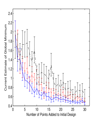
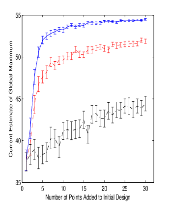
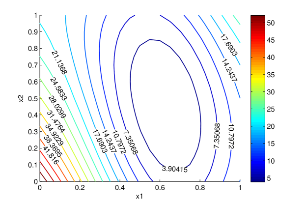
It is clear from Figure 3 that the optimization of the EI criterion using BNB (blue) leads to the true maximum in significantly fewer number of computer simulator runs compared to the (red) GA optimizer or baseline (black) search of a random maximin Latin hypercube. However the estimated global minimum does not seem to be significantly different for any of the optimization techniques, though on average BNB attains a closer estimate of the true minimum than GA which is in turn closer on average than the static method. This is somewhat intuitive as the Branin function is quite smooth and almost flat near the global minimum (see Figure 4).

Figure 4: Contours of Branin function in $[0,5]^{2}$ rescaled to $[0,1]^{2}$.

A comparison of a static design of size $n_{0}+k$ and the sequential design with EI (10) optimized using BNB and GA when estimating a contour of height $y=45$ is presented in Figure 5. Their performance is measured in terms of the divergence between the true and estimated contour, given by

$$d_{k}=\sqrt{\frac{1}{n}\sum_{i=1}^{m}(\hat{y}_{k}(x_{c,i})-a)^{2}},$$ (14)

where $\{x_{c,i},i=1,...,m\}$ denotes the discretized true contour at $y=45$, and $\hat{y}_{k}(\cdot)$ denotes the estimated process value after adding $k$ new points or from a static design of size $n_{0}+k$. The results are averaged over $100$ random maximin Latin hypercube initial designs of size $n_{0}=20$ each, and for each realization, we add $n_{new}=30$ additional trials.

Figure 5: Estimated BNB(blue), GA(red), and static(black) contour divergence versus number of new points added to initial design for the Branin test function.

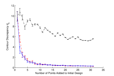
Figure 5 displays the divergence $d_{k}$ for the Branin function with contour at $y=45$. In this simulation BNB and GA methods perform similarly, both significantly better than the static design. The contour discrepancies of the sequential methods approach 0 quickly; an indication that this contour is relatively simple to locate. Since the contour at $y=45$ is in the very bottom left corner of the design region (see Figure 5), the maximin Latin hypercube design is less likely to place points very near the contour $y=45$, which results in poor performance for the static method.

Example 2 - Levy 2D. Suppose the computer model output $y=f(x_{1},x_{2})$ is generated using the Levy function given by

$$f(x_{1},...,x_{d})=\sin^{2}(\pi w_{1})+\sum_{k=1}^{d-1}(w_{k}-1)^{2}[1+10\sin^{2}(\pi w_{k}+1)]+(w_{d}-a)^{2},$$

where $w_{k}=1+(x_{k}-1)/4$ and $x_{k}\in[-10,10]$ for $k=1,...,d$. We rescale the inputs $x=(x_{1},...,x_{d})$ to $[0,1]^{d}$. For the two-dimensional Levy function (see Figure 6), the global maximum, $y_{max}=95.4$, and minimum, $y_{min}=0$, are attained at $(x_{1},x_{2})=(0,0)$ and $(x_{1},x_{2})=(0.55,0.55)$.

Figure 6: 2D Levy function contour plot rescaled to $[0,1]^{2}$

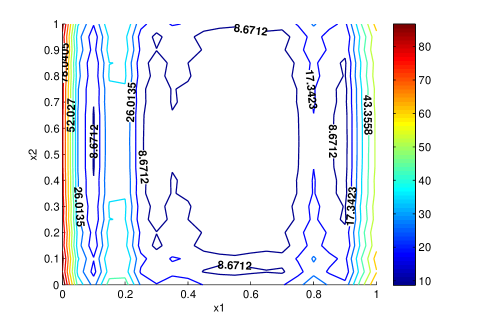
Figure 7 presents the long run comparison of the BNB and GA optimizers for maximizing the EI criterion (8) developed for simultaneous estimation of the global maximum and minimum. As in Example 1, the results are averaged over $100$ realizations with initial designs of size $n_{0}=20$ and $n_{new}=30$ additional trials. For this example, BNB is a clear winner and leads to better estimates of the global optima in much fewer simulator runs for both the maximum and minimum. As expected, GA performs significantly better than the static design.

(a) Minimum

(b) Maximum

Figure 7: Estimated optima for Levy 2D function (true minimum = 0, maximum = 95.4); BNB (blue - solid), GA (red - dashed), static (black - dash-dotted).

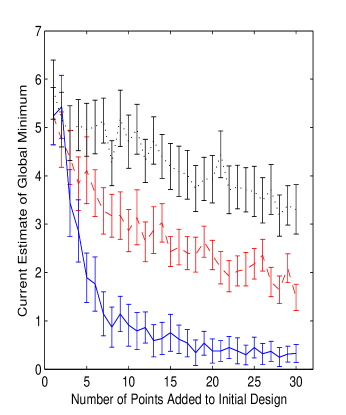
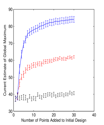
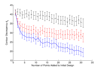
Figure 8 presents the divergence comparison of the sequential design with the two optimizers as well as a static design when estimating the contour at $y=70$. Here also, each initial design was of size $n_{0}=20$, $n_{new}=30$ new trials were added sequentially, and the results are averaged over $100$ initial random maximin Latin hypercube designs. As in the maximum and minimum case, the sequence of points added by the BNB (blue) optimization of EI (10) lead to quicker convergence of the contour divergence compared to GA (red). On average the static (black) designs provide relatively minimal improvement to the contour estimate.

Figure 8: Estimated contour divergence comparison for the 2D Levy function ($y=70$); BNB (blue - solid), GA (red - dashed) and static (black - dash-dotted).

Example 3 - Levy 4D. We now use an example of a simulator with four-dimensional inputs (Levy function) to demonstrate that careful optimization of the EI criterion can save significant amount of simulator runs. The simulation results use 30 initial design points chosen from random maximin Latin hypercube, and 20 additional points added sequentially. Comparisons using this higher dimensional function may highlight the differences between the two methods of optimization. BNB and GA were each given a budget of 3000 evaluations of the EI criterion. The true global maximum is approximately 255 at $(0,0,0,0)$, and the minimum is 0 at $(0.55,0.55,0.55,0.55)$.

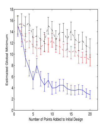
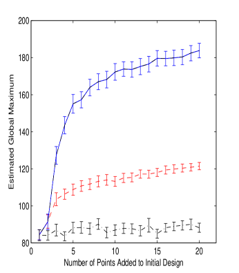
Figure 9 displays the comparison of our BNB algorithm with the GA and static designs in simultaneously estimating the maximum and minimum of the 4D Levy function. The results are averaged over 100 random maximin Latin hypercube initial designs of size $n_{0}=30$. BNB begins to locate both the minimum and maximum much more quickly than GA, which is in turn better than the static design. BNB is the only method that gets close to the maximum in 20 additional trials. All three methods are slow to locate the global maximum, a reflection of the complexity of the Levy function.

(a) Estimated Minimum

(b) Estimated Maximum

Figure 9: Estimated optima for Levy 4D function (true minimum = 0, maximum = 255); BNB (blue - solid), GA (red - dashed) and static (black - dash-dotted).

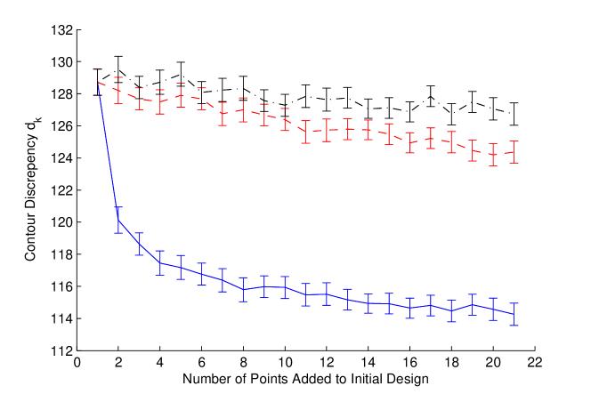
As before, we simulate the estimation of the $y=180$ contour of the 4D Levy function for BNB, GA, and static designs. The number of initial points $n_{0}$ was 30 and 20 new points were added. The results are averaged over 100 random maximin Latin hypercube designs. Figure 10 displays the contour divergence $d_{k}$ for the three designs - sequential with EI (10) optimized using BNB, GA and the static design. The new points selected by the BNB algorithm allow estimation of the 4D Levy $y=180$ contour more accurately than the other two methods, decreasing the contour divergence much more rapidly after only one point was added.

Figure 10: Estimated contour divergence comparison for the 4D Levy function ($y=180$); BNB (blue - solid), GA (red - dashed) and static (black - dash-dotted).

As illustrated in these examples, the branch and bound algorithm is quite competitive. For 2D and 4D Levy functions, BNB is superior to GA and static in estimation of contours as well as simultaneous estimation of the maximum and minimum. In estimating the maximum and minimum of the Branin function BNB locates the maximum much more quickly than the other methods, and all 3 methods are similar in estimating the minimum. For contours of the Branin function GA performs on par with BNB, both of which are preferable to a static design. The Branin function is relatively smooth, and hence optimization of EI criteria is relatively simple, which may explain the absence of differences between these methods in some cases.

5 Discussion

We have generalized the expected improvement criterion for finding the maximum and minimum (simultaneously) as the features of interest, and demonstrated the use of this infill criterion on the Levy and Branin test functions. Also we have developed branch and bound algorithms for contour and maximum/minimum estimation, compared them with genetic algorithms and static designs, and have shown that the BNB outperforms the other two optimization approaches. This study demonstrate that careful optimization of the EI criterion can save significant amount of simulator runs.

Note that we have used a ‘stochastic version’ of the BNB algorithm, and the approximation comes in from estimating the bounds of $\hat{y}(\mathbf{x})$, $\hat{s}(\mathbf{x})$ based on points in each rectangle $\mathcal{Q}\in\mathcal{Q}_{init}=[0,1]^{d}$. Further work should be done to investigate maximization of the proposed EI criteria using a non-stochastic branch and bound algorithm.

References

- (1)
- Balakrishnan et al. (1991) Balakrishnan, V., Boyd, S. and Balemi, S. (1991), ‘Branch and bound algorithm for computing the minimum stability degree of parameter-dependent linear systems’, Int. J. of Robust and Nonlinear Control 1(4), 295–317.
- Forrester and Jones (2008) Forrester, A. and Jones, D. (2008), Global Optimization of Deceptive Functions With Sparse Sampling, in ‘12 th AIAA/ISSMO Multidisciplinary Analysis and Optimization Conference’, American Institute of Aeronautics and Astronautics.
- Holland (1975) Holland, J. (1975), ‘Adaption in Natural and Artificial Systems’.
- Jones (2001) Jones, D. (2001), ‘A Taxonomy of Global Optimization Methods Based on Response Surfaces’, Journal of Global Optimization 21(4), 345–383.
- Jones et al. (1998) Jones, D. R., Schonlau, M. and Welch, W. J. (1998), ‘Efficient Global Optimization of Expensive Black-Box Functions’, Journal of Global Optimization 13(4), 455–492.
- Lawler and Wood (1966) Lawler, E. and Wood, D. (1966), ‘Branch-and-bound methods: A survey’, Operations research pp. 699–719.
- Mitchell (1996) Mitchell, M. (1996), An Introduction to Genetic Algorithms, Bradford Books.
- Moore (1991) Moore, R. (1991), ‘Global optimization to prescribed accuracy’, Computers & mathematics with applications(1987) 21(6-7), 25–39.
- Papalambros et al. (2002) Papalambros, P., Goovaerts, P. and Sasena, M. (2002), ‘Exploration of Metamodeling Sampling Criteria for Constrained Global Optimization’, Engineering Optimization 34(3), 263–278.
- Ranjan et al. (2008) Ranjan, P., Bingham, D. and Michailidis, G. (2008), ‘Sequential Experiment Design for Contour Estimation from Complex Computer Codes’, Technometrics 50(4), 527–541.
- Sacks et al. (1989) Sacks, J., Welch, W., Mitchell, T. and Wynn, H. (1989), ‘Design and analysis of computer experiments’, Statistical Science 4(4), 409–435.
- Santner et al. (2003) Santner, T. J., Williams, B. and Notz, W. (2003), The Design and Analysis of Computer Experiments, Springer.
- Sóbester et al. (2005) Sóbester, A., Leary, S. and Keane, A. (2005), ‘On the design of optimization strategies based on global response surface approximation models’, Journal of Global Optimization 33(1), 31–59.
- Stein (1999) Stein, M. L. (1999), Interpolation of Spatial Data: Some Theory for Kriging, Springer.
- Villemonteix et al. (2006) Villemonteix, J., Vazquez, E. and Walter, E. (2006), ‘An informational approach to the global optimization of expensive-to-evaluate functions’, Arxiv preprint cs.NA/0611143 .