Boolean delay equations on networks: An application to economic damage propagation

Abstract

We introduce economic models based on Boolean Delay Equations: this formalism makes easier to take into account the complexity of the interactions between firms and is particularly appropriate for studying the propagation of an initial damage due to a catastrophe. Here we concentrate on simple cases, which allow to understand the effects of multiple concurrent production paths as well as the presence of stochasticity in the path time lengths or in the network structure.

In absence of flexibility, the shortening of production of a single firm in an isolated network with multiple connections usually ends up by attaining a finite fraction of the firms or the whole economy, whereas the interactions with the outside allow a partial recovering of the activity, giving rise to periodic solutions with waves of damage which propagate across the structure. The damage propagation speed is strongly dependent upon the topology. The existence of multiple concurrent production paths does not necessarily imply a slowing down of the propagation, which can be as fast as the shortest path.

1 Introduction

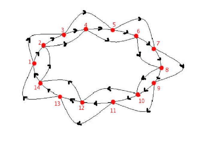
In most economic models, the production system is modeled as a unique representative producer (e.g., with the Cobb-Douglas function of the Solow model) or as a set of sectors, in which there is a unique representative producer by sector (e.g., in General Equilibrium Models). But the real production system can best be seen as a network composed of firms, producing different goods and services, and connected by suppliers and customer links. In such a network, the firm $j$ supplies a fraction of its production to other firms, that use this production as an input for their own production function (see [Fig. 1], for instance).

Introducing the role of networks in the economic system can lead to complex endogenous economic dynamics [1]. But the network formalism is also well adapted to study the cascade effects generated by exogenous events, positive in the case of new orders from the market [2, 3, 4, 5, 6, 7, 8] and negative in the case of financial crisis [9], random local strikes affecting production [10, 11], or natural disasters [12, 13, 14]. In classical economic models, where the production system is represented as a unique representative producer or as a small set of representative producers, indeed, exogenous events effects on the numerous firms have to be averaged over all firms, or over all firms of each sector. Because such effects are often highly heterogeneous, and because consequences and responses are highly nonlinear, this averaging process can bias the analysis, and makes it impossible to assess the consequences of an exogenous shock.

The case of natural disasters is particularly interesting, because disaster impacts are very heterogeneous and affect especially strongly a small set of firms [15, 16]. In such cases, the total economic impact of the catastrophe can be much higher than the direct impacts of the event, because indirect effects through supply chains can be large. For instance, an earthquake that destroys a bridge can cause losses that are much larger than the value of the bridge, because impacts on transportation costs and duration can impair production in many firms.

Such results have been reported using input-output models at the sector level [17, 18, 19, 13], or specific network models [20]. To account for heterogeneity at the firm level, an appropriate input-output formalism has been developed in [12, 13, 14], and used to analyze disaster consequences. This approach has demonstrated that the shape and the structure of the network play an important role in disaster vulnerability, justifying the introduction of network effects in the economic assessment of natural disasters. The purpose of the present manuscript is to simplify as much as possible the formalism, within the framework of Boolean Delay Equations (BDEs), to be able to go beyond the simple observation that the network structure has an influence on disaster consequences, and to analyze this dependency.

BDEs are semi-discrete dynamical systems, whose discrete variables evolve in continuous time; they have been introduced about 25 years ago [21, 22, 23], and they are related to the kinetic logic of Thomas [24]: nevertheless, in BDEs, the memory of the system can contain more and more information as the time goes on, allowing for solutions of increasing complexity, which hence display deterministic chaotic behavior, as it has been recently observed experimentally [25]. Apart from their intriguing mathematical properties, BDEs represent an useful tool in the modeling of complex systems, characterized by threshold behavior, multiple feedbacks, and distinct time delays. They have been in particular successfully applied to the study of climate dynamics [26], of earthquake physics [27, 28], and of real life problems [29, 30] (see [31] for a recent review). The present work is a first step towards the application of BDEs to phenomena in the economic realm and, at the same time, it deals with the clarification of the role played by stochasticity in these systems.

By using BDEs, we plan to take into account the importance of the topology of the network, and of the different delays involved in the production paths [2, 3, 4, 5, 7, 8], on the total losses due to the initial catastrophe. The manuscript will develop the role of the connectivity of the structure: how the multiplicity of products needed by each industry affects the vulnerability of the whole industry, and what are the effects of multiple production paths from one firm to down-stream production firms. We are specially interested by long term production shortage spatio-temporal patterns generated by the generic asynchrony due to variable time lengths of concurrent production paths.

Even though we are using Boolean variables to describe the production of individual firm, a zero value should not be interpreted in terms of a destruction of the production unity: we rather mean that some shortage has been generated through production interactions; similarly, a level of one simply implies that the firm has recovered from previous impairing of production. When taking instead the interpretation of the zero value as a complete destruction of the firm, our models could be interesting from the point of view of the study of damage spreading in an Operational Research framework. Finally, we will show that a macroeconomic quantity, measuring the density of fully active firms, allows to characterize the propagation of the consequences of the initial catastrophe in the various considered cases.

2 The models

A realistic representation of the economy at the firm level would make possible to assess both the direct and the indirect losses due to a catastrophic event, by taking into account also the backward and forward propagations of the event’s consequences, hence the failure avalanches and the ripple effects which move across the chains of suppliers and producers in the network. For instance, the analysis of the impacts on the regional economy of the Northridge earthquake [15, 32] makes it evident that a catastrophe can have very heterogeneous repercussions, and that the indirect losses due in particular to damages to the transport infrastructure system can be definitely higher than the direct losses themselves. Similar conclusions are obtained by the study of the consequences of the Loma Prieta and Northridge earthquakes [16], which underlines the importance of taking into account both the direct and the indirect losses, too; moreover this work shows that the repercussions can be less extended on firms belonging to a market larger than the strictly local one, hence suggesting to consider also economic models with adaptation (see, e.g., [20]).

Whereas the first steps towards a model suitable for realistic evaluations have been presented in [12, 13, 14], we introduce here some quite simplified toy models, which we will study within the framework of Boolean Delay Equations: the present approximation neglects some key ingredients, such as in particular the division in sectors of the economy, and the related observation that a given firm can usually choose between more providers of the same good, also in a strictly local economy. Nevertheless, with these over-simplifications, the numerically observed behaviors can be understood in detail from the theoretical point of view, and we find that our results are a good starting point for future analysis.

We take the Boolean variable $x_{i}(t)=0$ to mean that firm $i$ at time $t$ is impaired and can not fully produce (respectively, $x_{i}(t)=1$ implies that it is not impaired): this can be due both to the firm being itself damaged or to the fact that it lacks of the necessary inputs, since some of its suppliers (or some of the suppliers of its suppliers and so on) were previously damaged. Therefore, this simple modeling takes into account the role of the chains of suppliers and producers in real economies.

We study networks of $N$ firms, assumed to be placed on the vertexes of a directed graph defined by the connectivity matrix $A$. In our notation, $A_{ij}=1$ if part of the output of firm $j$ (the supplier) is needed as input for firm $i$ (the customer) and $A_{ij}=0$ otherwise. As a first step for assessing the losses due to the propagation of the consequences of a catastrophic event, hence the vulnerability of an economic network to a natural disaster, we analyze the vulnerability of the present models to the initial damage of a single firm. Therefore we will assume, without loss of generality, that the firm in the origin is initially destroyed during an interval of time of length $\tau_{c}$. We will look in particular at the dependence of the propagation of this event on the structure of the matrix $A$, hence on the resulting network topology, and at its dependence on the ensemble of the delays that exist in the economic system.

We consider both isolated networks, the free models, and networks interacting with the outside, hence economies with adaptation, the forced models. In the first cases, the availability $S_{ji}$ of the good manufactured by firm $j$ at firm $i$ is simply delayed from production $x_{j}$ with a constant time length $\tau_{i,j}$ according to:

$$S_{ji}(t)=x_{j}(t-\tau_{i,j})\hskip 21.68121pt\mbox{ free models.}$$ (1)

In the presence of adaptation, which means that the economy is not locally isolated but there is instead the availability of some external rescue input, the stock $S_{ji}$ is made again disposable after that the production of the firm $i$ has been impaired for a duration of time that we take, in a first approximation, still equal to $\tau_{i,j}$:

$$S_{ji}(t)=\overline{x}_{i}(t-{\tau}_{i,j})\vee x_{j}(t-{\tau}_{i,j})\hskip 21.68121pt\mbox{ forced models},$$ (2)

where $\vee$ is the OR operator and $\overline{(\cdot)}$ means the Boolean negation. These equations give the truth table reported in [Tab. 1].

$x_{i}$	$x_{j}$	$S_{ji}$	free models
0	0	0	$j$ and $i$ inactive, the stock can not be reconstituted
0	1	1	$j$ active and $i$ inactive, the good is stocked
1	0	0	$j$ inactive and $i$ active, the stock is finished
1	1	1	$j$ active and $i$ active, the stock is updated
$x_{i}$	$x_{j}$	$S_{ji}$	forced models
0	0	1	$j$ and $i$ inactive, the stock is supplied from outside
0	1	1	$j$ active and $i$ inactive, the good is stocked
1	0	0	$j$ inactive and $i$ active, the stock is finished
1	1	1	$j$ active and $i$ active, the stock is updated

Table 1: The output table of the stock $S_{ji}$ of a given product as Boolean function of the activities $x_{i},x_{j}$ of the customer firm $i$ and of the supplier firm $j$, in the free models described by Eq. (1) and in the forced models described by Eq. (2), respectively.

In our simple toy models, the production $x_{i}(t)$, of firm $i$ at time $t$, needs the presence of all the stocks of goods usually provided by the suppliers $\{j:A_{ij}\neq 0\}$ to which the firm $i$ is connected in the network. Besides, we assume that $x_{i}(t)$ also depends upon the value $\mu_{i}(t)$ of an external coefficient, which is an independent Boolean variable that allows in particular for the initial destruction of the firm in the origin. These constraints can be expressed, both for the free and the forced models, by the system of $N$ BDEs:

$$x_{i}(t)=\mu_{i}(t)\prod_{j=1}^{N}\overline{A}_{ij}\vee S_{ji}(t)\hskip 21.68121pt\mbox{ for }i=1,\dots,N.$$ (3)

Here the product $\prod$, which runs over all the sites of the network, means the Boolean operator AND, $\wedge$. The dependence on the delays $\{\tau_{i,j}\}$ is implicit, through the stocks, given by Eq. (1) or Eq. (2).

In order to get well defined solutions for this system, one has to fix the initial values of the set of variables $\{x_{i}(t)\}$ in the interval $[-\tau_{max},0]$, where $\tau_{max}$ is the largest possible delay. Moreover, one has to choose the behaviors of the external functions $\{\mu_{i}(t)\}$. We only study the simple cases in which the economy starts undamaged and all the external functions take the value one during the evolution, apart from the destruction of the single firm in the origin, i.e. on the node $i=1$. Notice that this firm is not definitely eliminated form the network: we assume instead that it is forced to stop the activity from the time $t=0$ up to the time $\tau_{c}$; this means $\mu_{1}(t)=0$ for $t\in[0,\tau_{c}]$.

We compare results for deterministic delays, chosen all equal to $\tau_{0}$, with those for the more realistic situation of random delays $\{\tau_{i,j}\}$, independently and uniformly distributed in the interval $[\tau_{min},\tau_{max}]$, with:

$${\cal P}(\tau_{i,j})=\frac{\tau_{min}}{\tau_{max}}\sum_{k=1}^{\tau_{max}/\tau_{min}}\delta\left(\tau_{i,j}/\tau_{min}-k\right),$$ (4)

i.e. the random variables are multiples of the unity of time fixed by $\tau_{min}$. We usually take $\tau_{0}=\tau_{min}=1$ day and $\tau_{max}=10$ days. Though the possibility of defining BDE systems characterized by random delays with a given probability distribution was already stated in [21], the present study is the first example in this direction to our knowledge.

Still, in the first part of this work we look at a deterministic braid chain network, corresponding to a connectivity matrix $A$ with circulant structure (see [Fig. 1]), whereas in the second part we study a directed random graph (DRG). We will consider in particular the family of directed random graphs, $D(N,p)$ [33, 34], obtained by generalizing the rule of the well known Erdős-Rényi undirected random graph (RG) [35, 36, 37], where each of the $N(N-1)$ directed links is present or absent with the same independent probability $p\in[0,1]$. Hence, the elements of the connectivity matrix $\{A_{ij}\}$ are random variables, assumed to be independently and identically distributed:

$${\cal P}(A_{ij})=\left\{\begin{array}[]{lcl}\delta\left(A_{ij}\right)&\mbox{ for }&i=j\\ p\delta\left(A_{ij}-1\right)+(1-p)\delta\left(A_{ij}\right)&\mbox{ for }&i\neq j\\ \end{array}\right.$$

The probability $p$ is straightaway related to the mean number of input-output connections (i.e. the in/out-degree), $z=\langle k_{in}\rangle=\langle k_{out}\rangle=(N-1)p\simeq Np$, of the resulting directed network.

In the considered context of BDEs with stochasticity, the delays $\{\tau_{i,j}\}$ and the elements of the connectivity matrix $\{A_{ij}\}$ are quenched random variables: when defining the BDE system one fixes their values, with probabilities given by Eq. (4) and Eq. (2), to a given disorder configuration, and they are assumed to be constant on the time scale of the evolution we are interested in.

	Fr, $\tau_{0}$	Fr, ${\cal P}(\tau_{i,j})$	Fo, $\tau_{0}$	Fo, ${\cal P}(\tau_{i,j})$
CM, $n=1$	3.2	3.3	3.6	3.6
CM, $n>1$	3.4	3.5	3.7	3.8
DRG	4.2	4.3	4.4	4.4

Table 2: We summarize here the main characteristics of the models studied in the following, and we indicate in each box the section where the model with all the corresponding details is discussed and the figures showing our results are presented. We label Fr the free models described by Eq. (1) and Fo the forced models obeying to Eq. (2); then, we look both at the case in which all the delays are deterministically taken equal to the same time unit $\tau_{0}$, and at the random delay one, with ${\cal P}(\tau_{i,j})$ defined by Eq. (4); still, CM refers to the deterministic braid chain network obtained from a circulant matrix, and DRG to the directed random graph, with ${\cal P}(A_{ij})$ given by Eq. (2); finally, we distinguish between single ($n=1$), and multiple ($n>1$), input-output connections in the braid chain, whereas the models defined on the DRG with average in/out-degree $z$ both smaller and larger then one are treated in the same sections.

With the aim of describing the solutions, and particularly their behaviors in the limit of a large number $N$ of variables, we find interesting to introduce a macroeconomic observable, that is to say the average density of firms which maintain their production, $\rho(t)$. In the deterministic case it is given by:

$$\rho(t)\equiv\frac{1}{N}\sum_{i=1}^{N}x_{i}(t).$$ (5)

In the presence of stochasticity, in the delays and/or in the elements of the connectivity matrix, the behaviors of the systems are better captured from the density averaged over disorder:

$$\langle\rho(t)\rangle\equiv\int\prod_{i,j}d\tau_{i,j}{\cal P}(\tau_{i,j})\int\prod_{h,k}dA_{hk}{\cal P}(A_{hk})\rho(t),$$ (6)

that can be computed numerically by considering an enough large number, ${\cal N}_{s}$, of different disorder configurations. We also look at the density averaged over a time window of length corresponding to the smallest possible delay, i.e. $\tau=\tau_{0}$ in the deterministic case and $\tau=\tau_{min}$ in the stochastic one:

$$\rho_{av}(t)\equiv\int_{t}^{t+\tau}\rho(s)ds.$$ (7)

Finally, in the considered simple toy models, the total number of impaired firms at time $t$, $\theta_{tot}(t)$, gives just the evaluation of the total losses due to the propagation at this time of the effects of the initial destruction of the single firm in the origin, hence it is also a measure of damage spreading:

$$\theta_{tot}(t)\equiv\sum_{i=1}^{N}\overline{x}_{i}(t).$$ (8)

Accordingly, the density can be straightaway obtained as:

$$\rho(t)=1-\frac{1}{N}\theta_{tot}(t).$$ (9)

When taking random delays and/or a random network structure, we study the average $\langle\theta_{tot}(t)\rangle$, defined analogously to the average density in Eq. (6).

We summarize in [Tab. 2] the different cases that we consider.

3 Circulant matrix

3.1 Topology

Here we look at the network topology corresponding to a braid chain, which is obtained from a connectivity matrix $A$ (of size $N\cdot N$) with circulant structure. When taking periodic boundary conditions for the indexes ($i\pm N\equiv i$), the elements can be written as:

$$A_{ij}=\left\{\begin{array}[]{ll}1&\mbox{ for }j=i-1,i-2,\dots,i-n\\ 0&\mbox{ otherwise},\\ \end{array}\right.$$ (12)

for some integer $n<N$. This models a directed braid chain, with the same in/out-degree $n$ for all the nodes. Each firm is linked to $2n$ other firms, and needs as inputs part of the goods manufactured by the previous $n$ ones (its suppliers), whereas the produced outputs are used from the next $n$ ones (its customers). The resulting deterministic topology is strongly connected: starting from any node one finds at least one directed path along which the signal can propagate to any other node, and in fact there are multiple concurrent paths as soon as $n>1$. Most of these paths have the same time length in the purely deterministic case of equal delays, whereas they have usually different time lengths for random delays. In other words, the random delays allow to model the asynchrony in the concurrent production paths. We present in [Fig. 1] an example for $n=2$ in/out-degree.

Figure 1: The braid chain structure given by a circulant matrix with periodic boundary conditions in the case of $n=2$ in/out-degree. The size of the network is $N=14$, and the nodes are arbitrarily ordered clockwise. In the deterministic case of equal delays also the choice of the origin (the $i=1$ node) is completely arbitrary. Note that instead, in the presence of stochasticity, the different concurrent paths connecting two given nodes do not usually have the same duration in time, although they might have the same spatial length in terms of number of steps along the chain.

When $A$ is a circulant matrix, the equation for the variable $x_{i}$ of the system (3) can be simplified into:

$$x_{i}(t) = \mu_{i}(t)\left[\prod_{j=1}^{n}x_{i-j}(t-\tau_{i,i-j})\right]$$ (13)

$$x_{i}(t) = \mu_{i}(t)\left[\prod_{j=1}^{n}\overline{x}_{i}(t-\tau_{i,i-j})\vee x_{i-j}(t-\tau_{i,i-j})\right],$$ (14)

for the free models defined by Eq. (1) and the forced models defined by Eq. (2), respectively. The considered systems give an extremely simplified description of the input-output structure of real economic network; nevertheless, braid chain structures turn out to be an interesting approximation when interpreting each node $i$, with its production $x_{i}$, as corresponding to a whole sector of the economy.

3.2 The free model with $n=1$ and equal delays

The free model on a braid chain network, with a single input-output connection for node, $n=1$, and deterministically taken delays all equal to the same time unit $\tau_{0}$, is an example of conservative system of BDEs [21, 22, 23, 31]. Its dynamics is periodic from the beginning for all the initial states, without any transient. The model is described by the set of equations:

$$x_{i}(t)=\mu_{i}(t)\>x_{i-1}(t-\tau_{0})\hskip 21.68121pti=1,\dots,N,$$ (15)

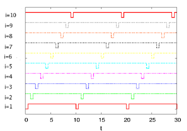
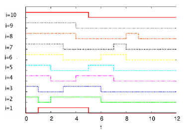
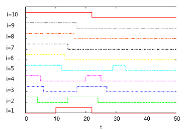
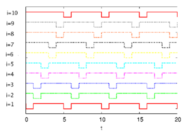
where we fix initial values $x_{i}(t)=1\>\forall i$ for $t\in[-\tau_{0},0)$, and we represent the initial destruction of the single firm on node $i=1$, for a duration $\tau_{c}$, by the choice of the external coefficient: $\mu_{1}(t)=0$ for $t\in[0,\tau_{c})$. The solution displays a wave of nodes taking the value zero the one after the other, which propagates periodically across the chain, as in the example given in [Fig. 2a].

Figure 2: Time evolution of the state of the 10 nodes of the free model on a braid chain, with $n=1$, after an initial perturbation of node $i=1$. Each Boolean variable $x_{i}(t)$ is plotted as function of $t$ and it is a piecewise constant function varying between 0 and 1. We moreover shift the solutions $x_{i}(t)$ along the $y$ axis, as a function of the node index $i$, for visualizing the propagating wave in the network. On the left, the delays are deterministically taken all equal to $\tau_{0}=1$ day, and the duration of the initial perturbation is $\tau_{c}=\tau_{0}/2=0.5$ day. On the right, we look at a particular configuration of random delays, $\{\tau_{i,i-1}\}$, uniformly distributed between $\tau_{min}$= 1 day and $\tau_{max}$=10 days, yielding a period of 47 days. Here the duration of the initial perturbation is $\tau_{c}=\tau_{min}=1$ day.

This simple system is analogous to the model introduced in [31] as a first step towards a BDE equivalent of hyperbolic partial differential equations. In that work, we were discretizing the unidimensional space lattice, and in the analogy the node index $i$ plays the role of the discretized coordinate. We studied the evolution starting from an initial state where only the variable associated to the lattice point in the origin was equal to one, and we found correspondingly a propagating wave of points taking the value one in the spatio-temporal pattern.

In fact, when the duration of the initial perturbation, $\tau_{c}$, is smaller than the unit of time, $\tau_{0}$, the role of the external coefficients can be absorbed into the initial conditions. The evolution shows in any case no transient and the period of the solution is ${\cal\pi}=N\tau_{0}$. For values of $\tau_{c}$ multiple of $\tau_{0}$, the density of firms which maintain their production takes the constant value $\rho(t)=1-{\tau_{c}}/(N{\tau_{0}})$, whereas more generally it has period $\tau_{0}$.

This dynamics implies that, on the one hand, the damage does not spread, but, on the other hand, the activity never recovers completely: each impaired firm gets back to the unaffected state after the time $\tau_{c}$, but contemporaneously its production shortage reaches its customer, with a constant delay $\tau_{0}$. This unrealistic result is linked to one of our simplifying assumptions, namely the discretization of firm production capacity, with no possibility for overproduction or production rescheduling.

3.3 The free model with $n=1$ and random delays

In the free model on a braid chain network with $n=1$, the effect of stochasticity in the delays can be straightaway worked out explicitly:

$$x_{i}(t) = x_{i-1}(t-\tau_{i,i-1})=$$ (16)

$$= x_{i-2}(t-\tau_{i,i-1}-\tau_{i-1,i-2})=\dots=$$

$$= x_{i}\left(t-\sum_{k=0}^{N-1}\tau_{i-k,i-k-1}\right).$$

Correspondingly, one finds that the solution is still periodic from the beginning for all the initial states, and the system is therefore once again conservative.

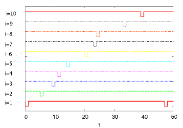
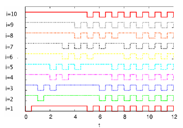
In the considered case of an initial perturbation of node $i=1$ of duration $\tau_{c}$, we get in particular a periodically propagating wave of nodes taking the value zero the one after the other in the spatio-temporal pattern, as in the deterministic case. The difference is that the propagation time of the perturbation, from a supplier $i-1$ to its customer $i$, is now given by the quenched random variable $\tau_{i,i-1}$, and the period $\pi$ of the solution, for a given disorder configuration, is equal to the sum of these delays along the whole chain (see [Fig. 2b]), with in average $\langle\pi\rangle=N\langle\tau_{i,i-1}\rangle=N(\tau_{max}+1)/2$.

Figure 3: Time plot of the average fraction of fully active firms, $\langle\rho(t)\rangle$, in the free model on a braid chain, with $n=1$, and stochasticity in the delays. Here $\tau_{max}=10$ days, as in [Fig. 2b], and we compare the behaviors for network sizes $N=10$, 20, 50 and 100 with the expected ones (see Appendix A). On the left we present the details at short times, and on the right the whole considered time window. The data are averaged over ${\cal N}_{s}$ different random configurations of the delays, a number which is taken enough large to give errors of the order of the point size in the plot.

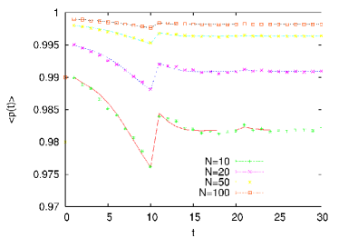
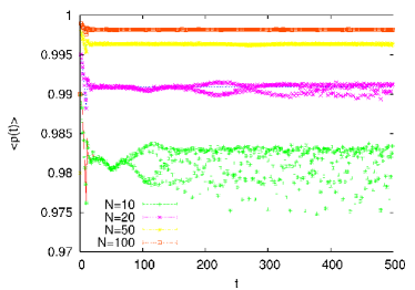
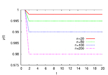
The density averaged over the disorder, $\langle\rho(t)\rangle$, can be computed analytically by applying the central limit theorem (see Appendix A). In [Fig. 3], we compare the expected behavior, given by Eq. (59), with the numerical results, for different network sizes $N$: at short times, one can observe the jumps at $t=\tau_{max}$; at long times, there are corrections to the expected behavior, since in the considered sums of random delays the same variables appear more than once; nevertheless, the mean asymptotic value is in agreement with Eq. (61).

The case $\tau_{c}\neq\tau_{min}$ can be understood within the same framework, and one finds that, for large $N$ values, the average density does only depend on the ratio of the duration of the initial damage, $\tau_{c}$, to the size of the network $N$ itself:

$$\langle\rho_{av}(t)\rangle\simeq 1-\frac{\tau_{c}}{N}\langle\theta_{tot}(\tau_{c}=1,t)\rangle.$$ (17)

Here we are looking at $\langle\rho_{av}(t)\rangle$, assumed to be averaged also over a time window of length $\tau_{min}=1$ day: in fact, for $\tau_{c}$ not multiple of $\tau_{min}$, the density $\langle\rho(t)\rangle$ approximately oscillates between the expected solution for $[\tau_{c}/\tau_{min}]$ and for $[\tau_{c}/\tau_{min}]+1$ (where $[y]$ means the integer part of $y$), with period $\tau_{min}$: this result becomes correct in the asymptotic large time limit.

3.4 The free model with $n>1$ and equal delays

Generally, the BDE systems which describe the free models on a braid chain, with $n$ input-output connections, can be reduced to closed sets of $n$ equations; these equations involve the products of only $n$ variables, corresponding to nodes in consecutive positions along the chain, but each variable appears more than once, at different times.

In particular, in the deterministic case of delays all equal to $\tau_{0}$, and taking $N$ multiple of $n$ for simplicity, one has:

$$x_{i}(t) = \prod_{k=N/n}^{N-n+1}x_{i+n-1}(t-k\tau_{0})\cdot x_{i+n-2}(t-k\tau_{0})\cdot...\cdot x_{i}(t-k\tau_{0})$$

$$x_{i+1}(t) = \left[\prod_{k=N/n}^{N-n+2}x_{i+n-1}(t-k\tau_{0})\cdot x_{i+n-2}(t-k\tau_{0})\cdot...\cdot x_{i+1}(t-k\tau_{0})\right]\cdot$$

$$\cdot \left[\prod_{k=N/n+1}^{N-n+2}x_{i}(t-k\tau_{0})\right]$$

$$... = ...$$

$$x_{i+n-1}(t) = \left[\prod_{k=N/n}^{N-n+2}x_{i+n-1}(t-k\tau_{0})\right]\cdot$$ (18)

$$\cdot \left[\prod_{k=N/n+1}^{N-n+2}x_{i+n-2}(t-k\tau_{0})\cdot...\cdot x_{i+1}(t-k\tau_{0})\cdot x_{i}(t-k\tau_{0})\right].$$

In this expression they are contained all the possible paths along which the information, here the damage due to the initial perturbation, can propagate across the network. The reduction is analogous to the one of systems of differential equations to systems of higher order equations depending upon a smaller number of variables.

As soon as the number of connections is $n>1$, the dynamics is dissipative [21, 22, 23, 31]: the asymptotically stable solution is the state in which the whole economy is attained by the consequences of the initial damage, $x_{i}\equiv 0\>\forall i$, and it is finally reached for any duration of this starting perturbation $\tau_{c}\geq\tau_{0}$ (see [Fig. 4]). This result can be qualitatively explained by noticing that the present economic models lack of flexibility, since the $n$ different inputs to a given firm are considered to be linked by AND logical operators. Besides, the system is isolated and the deterministic topology of the braid chain is strongly connected.

Figure 4: Time evolution of the state of the 10 nodes of the free model on a braid chain, with $n=2$, after an initial perturbation of node 1. We plot $x_{i}(t)$ as a function of $t$, the solutions corresponding to different node index $i$ being shifted along the $y$ axis in order to visualize the spatio-temporal pattern. Here all the delays are equal to $\tau_{0}=1$ day. On the left, the duration of the initial perturbation is $\tau_{c}=\tau_{0}=1$ day, whereas on the right we take $\tau_{c}=\tau_{0}/2=0.5$ days. See the text for details.

We analyze the dynamics of the model starting from a situation in which the impaired firms occupy nodes in consecutive positions along the braid chain: let us say that in the interval $[t,t+1)$ (in unity of $\tau_{0}$) there are $\theta_{tot}(t)=k$ impaired firms, i.e., $x_{i}(t)=0$ for $i\in[i_{m}(t),i_{M}(t)]$, where $i_{M}(t)=i_{m}(t)+k-1$ and $k\ll N$. At this point, it is helpful to imagine a clock, with the hour-hand marking the position of the impaired firm closest to the origin, $i_{m}(t)$, and the minute-hand marking the position of the one farthest from the origin, $i_{M}(t)$, at time $t$. One finds that both the hour-hand and the minute-hand move with constant velocities, given respectively by 1 and $n$, and therefore (as soon as $n>1$), the width of the set of firms which are unable to fully produce increases with constant velocity, given by $n-1$, or in other words the damage spreads to a total number of $n-1$ more firms at each subsequent time step.

In fact, at each time step $t^{\prime}=t+1$, the firms in the next $n$ positions after $i_{M}(t)$ will be impaired, since at least one of the stocks that they need is finished, hence $i_{M}(t+1)=i_{M}(t)+n$. The first firm in the sequence is instead the only one which recovers its unaffected state, all its suppliers being previously fully active, hence $i_{m}(t+1)=i_{m}(t)+1$. Correspondingly, one gets just $\theta_{tot}(t^{\prime})=\theta_{tot}(t)+(n-1)$. The same argument can be applied again, starting from the new sequence, and so on.

Following this analysis, the evolution will stop at the time $t_{trans}$, when the minute-hand reaches the hour-hand with one turn of advantage: the system has attained the asymptotically stable steady state $x_{i}\equiv 0\>\forall i$, and the activity can not fully recover at all. Notice that the result is unchanged if, in the last time step of the transient, the minute-hand surpasses the hour-hand, since $x_{i}=0$ describes a shortage in the production of firm $i$ aside from the number of stocks of goods which are not available. Moreover, during the transient, each firm can recover at most once.

Summarizing, $\theta_{tot}(t)$ is linearly increasing with $t$ up to reach the system size $N$; correspondingly, for an initial perturbation destroying the production of one firm for a duration $\tau_{c}=\tau_{0}=1$ day, $\rho(t)=1-{1}/{N}-({n-1})t/{N}$ for $t\lesssim t_{trans}$ and $\rho(t)=0$ for $t\geq t_{trans}$, where the length of the transient is straightaway given by:

$$t_{trans}\simeq\frac{N-1}{n-1}\tau_{0}.$$ (19)

When generalizing to durations of the initial event $\tau_{c}\neq\tau_{0}$, it is important to distinguish between:

• $\tau_{c}>\tau_{0}$: Here the clock-argument turns out to be valid after the first $\sim\tau_{c}/\tau_{0}$ time steps; therefore, at large times, the damage spreading velocity is constant and equal to $n-1$, and the asymptotic stable state is the one where all the firms are impaired.

• $\tau_{c}<\tau_{0}$: As shown by data in [Fig. 4b], here one can say that it is the behavior of the initially damaged firm,

  $$x_{1}(t)=\left\{\begin{array}[]{ccc}0&\mbox{ for }&t\in[0,\tau_{c})\\ 1&\mbox{ for }&t\in[\tau_{c},1),\end{array}\right.$$ (20)

  that spreads across the network, with constant velocity $n-1$; the asymptotic solution is periodic of period equal to the unit of time, $\tau_{0}$, with all the firms synchronously impaired only in the first $\tau_{c}$ part of each period; the density $\rho_{av}(t)$, averaged over the period, is linearly decreasing with time, in this case up to the asymptotic constant value $\tau_{c}/\tau_{0}$, reached after a transient of length given again by Eq. (19).

These results are confirmed by the analysis that we present in Appendix B, where $\theta_{tot}(t)$ is computed explicitly.

3.5 The free model with $n>1$ and random delays

We now consider the free model on a braid chain, with multiple $n>1$ input-output connections, in the presence of stochasticity in the delays. Here the $\{\tau_{i,j}\}$ are quenched independent random variables, taken uniformly distributed in the interval $[\tau_{min},\tau_{max}]$ accordingly to Eq. (4), and the unit of time is given by $\tau_{min}$, that we choose again equal to 1 day.

As usual, we look in particular at the behavior of the system after the destruction of the single firm in the origin for a duration $\tau_{c}$. For $\tau_{c}\geq\tau_{max}$, we expect the damage to spread all over the network. In fact, the damage can not spread more slowly than in the peculiar case in which all the delays are equal to $\tau_{max}$: it follows that the state $x_{i}\equiv 0\>\forall i$ is asymptotically stable also in the presence of stochasticity, and that it is surely reached, after a transient $t_{trans}$.

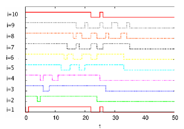
Nevertheless, now the concurrent paths, with the same space length along the chain, usually do no longer have the same time length, since in the sums of the involved delays appear different random variables. The presence of asynchrony has multiple consequences (see [Fig. 5]): the reduced set of equations (18) does generally contain a number of terms increasing with the path space lengths; during the dynamics, there is often no more a sequence of consecutive positions along the chain all occupied by impaired firms; as soon as $\tau_{c}<\tau_{max}$, each firm can be impaired and recover more than once; most intriguingly, because of this reason, the dynamics can be ruled by a faster time scale than the average delay.

Figure 5: Time evolution of the state of the 10 nodes of the free model on a braid chain, with $n=2$, after an initial perturbation of node 1. As in the previous cases, we plot $x_{i}(t)$ as a function of $t$ and we shift the solutions corresponding to different node index $i$ along the $y$ axis in order to visualize the spatio-temporal pattern. We look at a particular configuration of random delays, $\{\tau_{i,j}\}$, uniformly distributed between $\tau_{min}$= 1 day and $\tau_{max}$=10 days. The duration of the initial perturbation is $\tau_{c}=\tau_{min}$ on the left, and $\tau_{c}=\tau_{max}$ on the right, which yield transients of length 35 and 33, respectively.

In fact, since the delays are independent identically distributed random variables along the whole chain, in the limit $1\ll t\ll t_{trans}$, one can argue that the damage spreads with constant average velocity $\alpha$, where $\alpha_{min}\leq\alpha\leq\alpha_{max}$: the lower (respectively upper) limit is easily obtained by taking all the delays equal to $\tau_{min}$ (respectively to $\tau_{max}$), hence:

$$\frac{n-1}{\tau_{max}}\leq\alpha\leq n-1.$$ (21)

Nevertheless, as we are going to discuss, the upper limit is usually a definitely better approximation to the average velocity than the lower one.

In order to understand this point, we use once again the analogy with a clock, where here the hour-hand marks the position $i_{m}(t)$ of the impaired firm nearest to the origin and the minute-hand the position $i_{M}(t)$ of the impaired firm farthest from the origin: the key ingredients are that the network is braid chain structured and that the firm is affected by the consequences of the initial event, being unable to fully produce, as soon as a single one of the $n$ stocks that it needs is unavailable. Therefore, in the long time limit, for $1\ll\tau_{max}\ll n\ll N$, the average velocity of the hour-hand is negligible, $\langle i_{m}(t)\rangle\sim const$, and the most of the region between the origin and the minute-hand position, $i_{M}(t)$, is occupied by impaired firms, $\langle\theta_{tot}(t)\rangle\sim\langle i_{M}(t)\rangle-const$. In other words, the long term dynamics is dominated by the hare, moving more quickly than the average runner.

In this limit, one can moreover evaluate how far does the hare go in one time step, of length $\tau_{min}=1$, hence the approximated average velocity $\alpha^{*}$ of the signal: from a given supplier $j$, the damage can spread up to the farthest customer $i$ with $\tau_{i,j}=1$ delay value; at most, it can move up to $i=j+n$, with probability ${\cal P}(\tau_{j+n,j}=1)=1/\tau_{max}$. Generally, the probability that it moves of a distance at most $k$ is obtained by taking $\tau_{h,j}>1$ for $h=j+n,j+n-1,\dots,j+k+1$ and $\tau_{j+k,j}=1$. To get the average distance, one has to sum up each possible value $k=0,1...n$, multiplied for its corresponding probability, implying that $i=j+k$ is the farthest reachable point; hence it follows:

$$\alpha^{*}=\sum_{k=0}^{n}\frac{k}{\tau_{max}}\left(1-\frac{1}{\tau_{max}}\right)^{n-k}\simeq n-(\tau_{max}-1),$$ (22)

where we used the expansions:

$$\sum_{k=0}^{\infty}\epsilon^{k} = \frac{1}{1-\epsilon},$$

$$\sum_{k=0}^{\infty}k\>\epsilon^{k} = \epsilon\>\frac{d}{d\epsilon}\frac{1}{(1-\epsilon)},$$ (23)

with $\epsilon=(1-1/\tau_{max})$.

This result is still an underestimation of the effective average velocity in the considered limit, since there are corrections of order $\epsilon^{n}$ which make $\alpha$ larger, and we are moreover neglecting that the signal can go still faster on more than one time step. However, notice that, in a large region of the parameter values, one finds $\alpha^{*}>(n-1)(\tau_{max}+1)/\tau_{max}$, thereby confirming that the dynamics is usually dominated by a faster time scale than the one corresponding to the average delay.

A different approach is worked out in Appendix B, where the average number of impaired firms is explicitly computed as a function of the probability for the signal to have propagated of $k$ position in $t$ time steps: this analysis confirms the expectation of a linear behavior on a large time window, and it allows to predict the effective slope.

Figure 6: The average density of fully active firms, $\langle\rho(t)\rangle$, as a function of time, in the free model on a braid chain, after an initial perturbation of node 1 of duration $\tau_{c}=\tau_{min}$. Here the network size is $N=10000$, and the number of input-output connections is $n=20$; the average is taken over ${\cal N}_{s}=100$ different configurations of the disorder. We study delays depending only upon the customers, $\tau_{i,j}=\tau(i)\>\>\forall j$, only upon the suppliers, $\tau_{i,j}=\tau(j)\>\>\forall i$, and upon both of them, $\tau_{i,j}=\tau(i,j)$; in all of the cases they are independent random variables, identically uniformly distributed according to Eq. (4), with $\tau_{min}=1$ day and $\tau_{max}=10$ days. We compare the data with the lower ($\alpha=n-1$), with the upper ($\alpha=\alpha^{*}=n-(\tau_{max}-1)$) limits on the behavior, and with the prediction obtained by the approach explained in Appendix B. See the text for details.

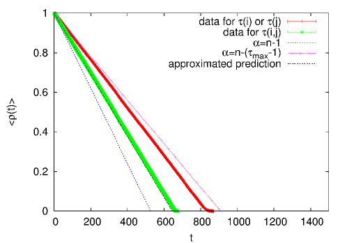
We present in [Fig. 6] our results on the average density of fully active firms, $\langle\rho(t)\rangle$, which is in fact linearly decreasing with time on a large window. The obtained behavior is well in agreement with our expectation, since the data lie between the lower limit $\rho_{min}(t)\sim 1-(n-1)t/N$, corresponding to the peculiar case in which all the delays are equal to $\tau_{min}$, and the upper limit $\rho_{max}(t)\sim 1-\alpha^{*}t/N$, evaluated using the hare argument. Moreover, the approach worked out in Appendix B allows to get results on $\langle\rho(t)\rangle$ which are nearly indistinguishable from numerical data.

Here we also consider delays depending only upon the customers, $\tau_{i,j}=\tau(i)\>\>\forall j$, or only upon the suppliers, $\tau_{i,j}=\tau(j)\>\forall i$, where $\{\tau(i)\}$ (respectively $\{\tau(j)\}$) are, as usual, independent identically distributed random variables, which follow the law Eq. (4): we get the same, slightly slower, average signal velocity in these last two cases. This result can be qualitatively explained by the observation that here there is a smaller number of propagation paths of different time lengths.

We found the same kind of almost linear decay, with velocity quite correctly approximated by $\alpha^{*}$, also for different values of the model parameters. We moreover checked that, as soon as $\tau_{c}\geq\tau_{min}$, the average density shows a dependence on $\tau_{c}$ only on the first $\sim\tau_{c}$ time steps. Finally, we studied the behavior of the densities $\rho(t)$ obtained from single different disorder configurations: this quantity does usually slightly fluctuate around the average value. In particular, the probability distributions of the transient length $t_{trans}$ is Gaussian-shaped, becoming rapidly peaked for increasing network size $N$: this means that most of the configurations of the delays gives a solution which reaches the asymptotic one, $x_{i}\equiv 0\>\forall i$, in about the same time, of order $t_{trans}\sim\alpha^{*}/N$. In other words, the density and $t_{trans}$ are self-averaging quantities, whose values are independent on the particular disorder configuration in the $N\rightarrow\infty$ limit.

Anyway, from the point of view of the dependence of the asymptotic solution upon the disorder, it is interesting to notice that the steady state $x_{i}\equiv 0\>\forall i$ is surely reached only for $\tau_{c}\geq\tau_{max}$: otherwise, there are configurations of the delays in which the smallest variable is $\min_{i,j}\{\tau_{i,j}\}=\tau^{*}>\tau_{c}$ and, for the same argument that we discuss in the deterministic case when $\tau_{c}<\tau_{0}$, the asymptotic solutions in these cases turn out to be periodic of period $\tau^{*}$, with all the firms simultaneously impaired in the first part of length $\tau_{c}$ of the period.

Nevertheless, since the probability of obtaining a configuration of the delays in which $\min_{i,j}\{\tau_{i,j}\}=\tau^{*}$, ${\cal P}_{\tau^{*}}$, approaches rapidly zero for increasing $N$ values, in the limit of large network size $N$, periodic asymptotic solutions are usually found only when the duration of the initial damage $\tau_{c}$ is smaller than the smallest possible nearest neighbor time length, $\tau_{min}=1$. In fact, this probability ${\cal P}_{\tau^{*}}$ can be straightaway evaluated:

$${\cal P}_{\tau^{*}}=\left(1-\frac{\tau^{*}-1}{\tau_{max}}\right)^{N^{2}}\mbox{ for }\tau_{min}\leq\tau^{*}\leq\tau_{max},\>\tau^{*}\in\mathbb{N}.$$ (24)

3.6 The forced models with $n=1$

We now turn onto the study of the forced models on a braid chain, defined accordingly to Eq. (14). When the in/out degree is $n=1$, and the delays are deterministically chosen all equal to $\tau_{0}$, the BDE system (3) can be reduced to the equation:

$$x_{i}(t)=\left\{\sum_{k=0}^{N-1}\overline{x}_{i-k}\left[t-(k+1)\tau_{0}\right]\right\}\vee x_{i}(t-N\tau_{0}),$$ (25)

where also the sum in the parenthesis is to be interpreted in the sense of the OR Boolean operator, $\vee$. For randomly distributed delays the equation is slightly more complex:

$$x_{i}(t)=\left[\sum_{k=0}^{N-1}\overline{x}_{i-k}\left(t-\sum_{j=0}^{k}\tau_{i-j,i-j-1}\right)\right]\vee x_{i}\left(t-\sum_{j=0}^{N-1}\tau_{i-j,i-j-1}\right),$$ (26)

since the time lengths of the paths are here given by the sums of the corresponding random variables.

Figure 7: Time evolution of the state of the 10 nodes of forced models on a braid chain, with $n=1$, after an initial perturbation of node 1. We plot $x_{i}(t)$ as a function of $t$ and we shift the solutions corresponding to different node index $i$ along the $y$ axis in order to visualize the spatio-temporal pattern. On the left we present data for the deterministic case of delays all equal to $\tau_{0}=1$ day, whereas on the right we look at a particular configuration of random delays $\{\tau_{i,j}\}$, uniformly distributed between $\tau_{min}=1$ day and $\tau_{max}=10$ days, with $\min_{i}\tau_{i,i-1}=\tau^{*}=\tau_{min}$. The duration of the initial damage is taken to be $\tau_{c}=2\tau_{0}=2$ days and $\tau_{c}=\langle\tau_{i,j}\rangle=5.5$ days, respectively. See the text for details.

One can distinguish between:

• A duration of the initial damage $\tau_{c}$ smaller than the smallest nearest neighbor propagation path, which means:

  • $\tau_{c}\leq\tau_{0}$ in the deterministic model;

  • $\tau_{c}\leq\min_{i,j}\{\tau_{i,j}\}=\tau^{*}$ in the stochastic one, where the probability to have $\tau^{*}>\tau_{min}$ is given by Eq. (24), and becomes negligible in the limit of large system size.

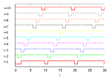
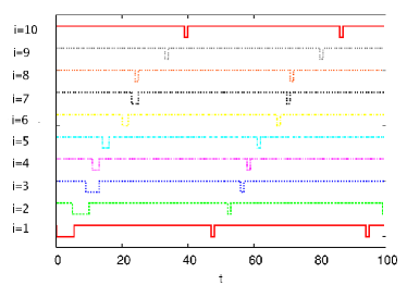
  Here the systems are conservative and the solutions are the same as in the corresponding free models (see [Fig. 2]). In particular, they are periodic from the beginning, with a wave of impaired firms which propagates in the spatio-temporal pattern. The periods are given by the sums of the delays along the whole chain, hence:

  • $\pi=N\tau_{0}$ in the deterministic case;

  • $\pi=\sum_{i=1}^{N}\tau_{i,i-1}$, with $\langle\pi\rangle=N(\tau_{max}+1)/2$, in the stochastic one.

• A duration of the initial damage $\tau_{c}$ larger than the smallest nearest neighbor propagation path ($\tau_{c}>\tau_{0}$ or $\tau_{c}>\tau^{*}$ in the deterministic or stochastic model, respectively). As shown in [Fig. 7], here the solutions are not periodic from the very beginning. In detail, when the firm in position $i$ is reached by the wave of damage, its activity is affected for a duration:

  • no longer than $\tau_{0}$ in the deterministic case,

  • no longer than $\tau_{i,i-1}$ in the stochastic one.

  The asymptotic solutions are surely reached after a first cycle in which each firm is impaired and recovers once. Moreover:

  • they are the same as for $\tau_{c}=\tau_{0}$ in the deterministic model,

  • they are the same as for $\tau_{c}=\tau^{*}$ (usually equal to $\tau_{min}$ in the large size limit), in the stochastic one.

3.7 The deterministic forced model with $n>1$

The behavior of the forced models on a braid chain, with in/out-degree $n>1$, can be understood in detail when the delays are deterministically taken all equal to $\tau_{0}$. Here, Eq. (14) simplifies into:

$$x_{i}(t)=\mu_{i}(t)\overline{x}_{i}(t-\tau_{0})\vee\left[\prod_{j=1}^{n}x_{i-j}(t-\tau_{0})\right].$$ (27)

Therefore, the firm $i$ maintains its production, as usual, if all its suppliers were fully active at the previous time step, but also if some of them were impaired and $i$ itself was already impaired: the production is recovered after one time step of length $\tau_{0}$.

Figure 8: On the left, we present the time evolution of the state of the 10 nodes of the deterministic forced model on a braid chain, with $n=2$, after an initial perturbation of node 1. As in the previous considered cases, we plot $x_{i}(t)$ as a function of $t$ by shifting the solutions corresponding to different node index $i$ along the $y$ axis. On the right, we show the density of fully active firms as a function of time in the same model, for a network size $N=10000$, and different values of the input-output connections $n$. In both of the cases we take a duration of the initial damage $\tau_{c}=\tau_{0}=1$ day.

Let us take for simplicity $N$ multiple of $n$, and let us start by considering a duration of the initial damage $\tau_{c}\geq\tau_{0}$: then, after the first time step, there are $n$ firms in consecutive positions along the chain which activity is simultaneously impaired; at the subsequent time step, these firms recover but the damage propagates to the next $n$ ones.

In other words, in this model, as soon as $t>1$, both the hour-hand and the minute-hand move with the same constant velocity $n$: the damage does not spread, but the activity never recovers completely. Correspondingly, the asymptotic solution is periodic of period $N/n$ and the density is just $\rho(t)=1-n/N$, as shown by the data presented in [Fig. 8].

Though here there is no complete breakdown of the economy, this simple case makes evident that, in the considered models, the presence of more connections does lead to a less favorable final outcome, with more impaired firms. This result can be explained by the fact that more connections do not lead to risk sharing, since having one impaired supplier is enough to stop a firm production. This assumption amounts to say that each supplier of a firm provides a different type of goods or services, and that one supplier cannot compensate for the loss of another supplier. In such a situation, a firm that is connected to more suppliers has higher risks of being indirectly affected by a shock.

When $\tau_{c}<\tau_{0}$, one still finds a propagating wave of $n$ impaired firms in consecutive position along the chain; nevertheless, here their activity is simultaneously impaired only in the first part of length $\tau_{c}$ of the time step. The situation is similar to the one encountered in the same case in the free models with $n=1$, i.e. it is the behavior of the initially attained firm (see Eq. (20)) which propagates along the network.

3.8 The stochastic forced model with $n>1$

Figure 9: Time evolution of the state of the 10 nodes of the stochastic forced model on a braid chain, with $n=2$, after an initial perturbation of node 1. We plot $x_{i}(t)$ as a function of $t$ by shifting the solutions corresponding to different node index $i$ along the $y$ axis in order to visualize the spatio-temporal pattern. As usual, we look at a particular configuration of random delays, $\{\tau_{i,j}\}$, uniformly distributed between $\tau_{min}$= 1 day and $\tau_{max}$=10 days. The duration of the initial perturbation is $\tau_{c}=\tau_{min}$. Notice that the solution does not display any periodicity in the considered time window.

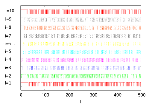
In the presence of stochasticity in the delays, the dynamics of the forced models on a braid chain, with $n>1$ input-output connections, turns out instead to be quite complex. Here we take as usual random independent delays, uniformly identically distributed according to Eq. (4), with $\tau_{max}=10$, in the unit of time given by $\tau_{min}=1$ day. The solution for a typical disorder configuration, after an initial damage of duration $\tau_{c}=\tau_{min}$, is shown in [Fig. 9]: intriguingly, despite of the relatively small network size considered, $N=10$, and of the small $n=2$ value, one does not observe any periodicity in the considered time window.

Since the delays are integer multiple of $\tau_{min}$, the asymptotic solution of the system (3), for a given disorder configuration, is surely constant or periodic because of general results on BDEs [21, 22, 23, 31]. Nevertheless, in the same works it is shown that, for irrationally related delays, BDEs can have solutions of increasing complexity, which display a number of jumps in time intervals of the same length increasing with time; this peculiar behavior is observed in particular in the case of linear systems such as the simple example:

$$x(t)=x(t-\tau)\bigtriangledown x(t-1).$$ (28)

Here, $\tau\in(0,1)$ is irrational, and $\bigtriangledown$ means the XOR Boolean operator, hence $x(t)$ is true ($x(t)=1$) only if a single one among the two variables $x(t-\tau)$ and $x(t-1)$ is true. It can moreover be shown that these aperiodic solutions can be approximated with the desired accuracy, for increasingly long times, by the periodic solutions of nearby BDEs systems with rationally related delays, which approximate better and better the irrational ones.

Though a careful analysis would be necessary in order to extend these results to the present case, we notice that Eq. (14), describing the model, is equivalent to:

$$\overline{x}_{i}(t)=\mu_{i}(t)\left\{\sum_{j=1}^{n}{x}_{i}(t_{ij})\bigtriangledown\overline{x}_{i-j}(t_{ij})\bigtriangledown\left[\overline{x}_{i}(t_{ij})\cdot x_{i-j}(t_{ij})\right]\right\},$$ (29)

where we label $t_{ij}=t-\tau_{i,i-j}$. The equivalence is due to the Boolean relation $\overline{a\vee b}=\overline{a}\wedge\overline{b}=\overline{a}\bigtriangledown\overline{b}\bigtriangledown(\overline{a}\cdot\overline{b})$, and it makes clear that the considered system is partially linear. This suggests that the long periods observed in the behavior of the solutions can be related to the known results on the existence of small, partially linear BDEs, with rationally related delays, which approximate the increasingly complex solutions of systems with irrationally related delays.

In order to better characterize our numerical findings, we find interesting to study various quantities:

• The length of the transient, $T_{trans}$, rigorously defined just as the time elapsed before that periodicity settles in. In the previously considered stochastic free models, $T_{trans}$ is the same as the time $t_{trans}$, which the average density takes to reach the asymptotic zero value. Instead, as we are going to discuss, in the present case one finds $T_{trans}\gg t_{trans}$, and it is therefore important to distinguish between the different meanings of the two transients.

• The period $\pi$ of the asymptotic solution itself, possibly equal to zero if it is constant.

• The period-averaged asymptotic density of fully active firms, $\rho_{\infty}$, defined as

  $$\rho_{\infty}=\frac{1}{\pi}\int_{T_{trans}}^{T_{trans}+\pi}\rho(t)dt.$$ (30)

Figure 10: Data on the forced model on a braid chain with random delays, uniformly distributed between $\tau_{min}=1$ day and $\tau_{max}=10$ days. Here we study the solutions of small systems of $N\sim 10$ equations with $n=2$, after an initial perturbation of node 1 of duration $\tau_{c}=\tau_{min}$. The results are obtained from ${\cal N}_{s}=1000$ different disorder configurations. On the left we plot the probability distribution of the transient, $P(T_{trans})$, in the center the probability distribution of the period, $P(\pi)$, and on the right the probability distribution of the period-averaged asymptotic density of fully active firms, $P(\rho_{\infty})$. Both $P(T_{trans})$ and $P(\pi)$ are presented in log-log scale, in order to make evident that they are not negligible also at very large values. See the text for details.

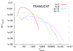
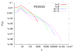
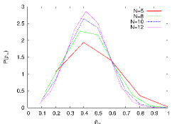
These quantities can be straightaway exactly measured up to relatively small system sizes $N\sim 12$. We present in [Fig. 10] our results on their probability distributions, $P(T_{trans})$, $P(\pi)$, and $P(\rho_{\infty})$ respectively, as obtained by considering ${\cal N}_{s}=1000$ different configurations of the random delays.

The most striking feature displayed by the data is that both the transient, $T_{trans}$, and the period, $\pi$, of the solution can increase very fast with the network size $N$. In order to make it evident, we have plotted the resulting probability distributions in log-log scale (see [Fig. 10a] and [Fig. 10b]): for instance, $P(T_{trans})$ is not negligible for values of the transient as large as $T_{trans}\sim 10^{6}$ (in units of $\tau_{min}$), in systems of $N=12$ nodes. In detail, we found that the average transient diverges exponentially with $N$, $\langle T_{trans}\rangle\propto\exp(constN)$, and that, at least for the considered $N$ values, the average period $\langle\pi\rangle$ displays a similar behavior.

The data on the asymptotic density of fully active firms, $\rho_{\infty}$, averaged over the disorder dependent period $\pi$, are shown in [Fig. 10c]: its probability distribution, $P(\rho_{\infty})$, turns out to be bell-shaped, and it becomes more peaked around the mean value for increasing network size $N$, therefore suggesting that the quite complex dynamics does not imply the unpredictability of the behavior of macroscopic intensive quantities, at least in the large network size limit.

In fact, whereas to predict the details of the solutions for given disorder configurations of the random delays seems to be a quite hard task, one can use an approach similar to the one of Section 3.5 to obtain the expected behavior of various average quantities.

For simplicity, we limit the analysis to the case in which the duration of the initial damage is not smaller than the smallest nearest neighbor propagation path, $\tau_{c}\geq\tau_{min}$. In the present extension of the clock argument, we assume that the minute-hand marks the position $i_{M}(t)$ of the firm farthest from the origin, i.e. from the node where the initial damage acted, which has already been impaired at least for a duration $\tau_{min}$ at time $t$. We recall that the network is braid chain structured and that the production of a given firm, apart from the initially damaged one, is impaired for the first time as soon as one of the $n$ stocks that it needs is unavailable. For these reasons, in the limit $1\ll\tau_{max}\ll n\ll N$, at large $t$, the signal is propagating across the chain with velocity still well approximated by Eq. (22):

$$\langle i_{M}(t)\rangle\sim\alpha^{*}t=[n-(\tau_{max}-1)]t.$$ (31)

The main difference with the previous stochastic free model is that here, because of the external rescue inputs, only a fraction $s^{*}$ of the firms between the origin and $\langle i_{M}(t)\rangle$ remains in average impaired during the time step of length $\tau_{min}$. Since the delays are taken independently and identically distributed along the whole chain, at large enough times this fraction is constant, and the damage spreads, up to invade the whole network, according to:

$$\langle\theta_{tot}(t)\rangle\sim s^{*}\alpha^{*}t=s^{*}[n-(\tau_{max}-1)]t,\mbox{ for }1\ll t{\lesssim}t_{trans}.$$ (32)

Correspondingly, the average density of fully active firms is again linearly decreasing with $t$, up to the time $t_{trans}$, at which it reaches a nearly constant asymptotic value:

$$\langle\rho(t)\rangle\sim\left\{\begin{array}[]{lcl}1-({s^{*}}/{N})\alpha^{*}t,&\mbox{ for }&1\ll t{\lesssim}t_{trans}\\ 1-{s^{*}},&\mbox{ for }&t\geq t_{trans}.\end{array}\right.$$ (33)

Hence, the effective transient, $t_{trans}$, relates to dynamics of $\langle\rho(t)\rangle$; in fact, it is the time at which the minute-hand reaches again the origin after a whole tour, and it is therefore of the same order as the time before that the density became zero, since the system attained the asymptotically stable configuration, $x_{i}\equiv 0\>\forall i$, in the stochastic free model:

$$t_{trans}\sim\frac{N}{\alpha^{*}}=\frac{N}{n-(\tau_{max}-1)}.$$ (34)

Therefore, whereas in the free model one has $t_{trans}=T_{trans}$, in the forced case it is important to distinguish between the transient $T_{trans}$, rigorously defined as the time elapsed before that periodicity settles in, that, as we showed numerically, is in average exponentially increasing with the network size $N$, and the definitely smaller effective transient $t_{trans}$, which can be more generally defined as the time at which macroscopic observables attain nearly constant average values.

Figure 11: The density of fully active firms $\rho(t)$ as a function of time, in the forced model on a braid chain with random delays, uniformly distributed between $\tau_{min}=1$ day and $\tau_{max}=10$ days, after an initial perturbation of node 1 of duration $\tau_{c}=\tau_{min}$. The network size is $N=10000$ and the in/out-degree is $n=20$. The results are for a single (typical) disorder configuration. We study delays depending only upon the customers ($\tau_{i,j}=\tau(i)\>\>\forall j$), delays depending only upon the suppliers ($\tau_{i,j}=\tau(j)\>\>\forall i$), and delays depending upon both of them ($\tau_{i,j}=\tau(i,j)$). See the text for details.

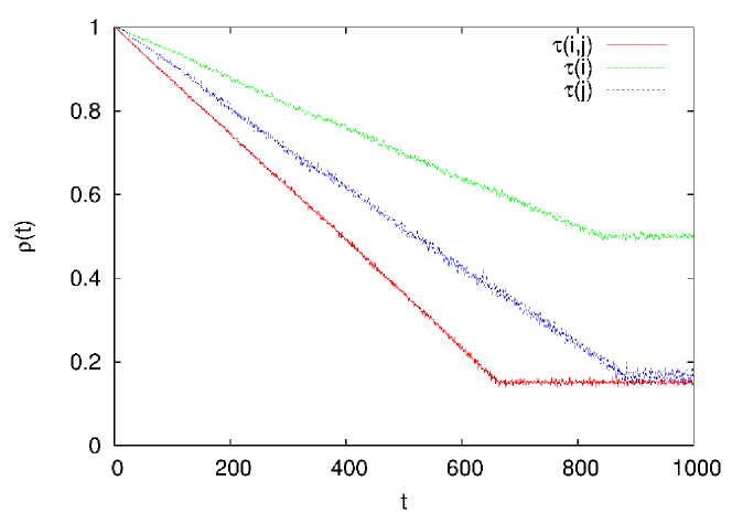
We present in [Fig. 11] the observed behavior of the density of fully active firm as a function of time, after an initial perturbation of node 1 of duration $\tau_{c}=\tau_{min}$, for a large network size $N=10000$ and in/out-degree $n=20$. In agreement with the picture emerging from the previous discussion, we find a nearly linear decay on a quite large time window, followed by small oscillations around the asymptotic value, which is reached in a time $t_{trans}$ of the same order of the estimation of the effective transient, $t_{trans}\sim 900$ (in units of $\tau_{min}$), that one gets from Eq. (34). From this point of view, we also recall that our evaluation of $\alpha^{*}$ is an underestimation of the damage spreading velocity, hence the corresponding value of $t_{trans}$ is to be considered an upper limit.

The data are for a single, typical, disorder configuration, in order to make evident that the fluctuations of $\rho(t)$ around the average are small, as it can be expected for a macroscopic intensive quantity: we checked in particular that both the effective transient length, $t_{trans}$, and the asymptotic mean value of the density, $1-s^{*}$, are usually the same for different choices of the random variables.

Besides considering delays depending both upon the customers and the suppliers, we present, in the same [Fig. 11], data on the system with delays depending only upon the customers, $\tau_{i,j}=\tau(i)\>\>\forall j$, or only upon the suppliers, $\tau_{i,j}=\tau(j)\>\>\forall i$: the last two cases are characterized by compatible values of the effective transient, $t_{trans}$, which is slightly larger than in the first one. This can be explaining by noticing that, as in the stochastic free model, when $\tau_{i,j}$ depend on both of the indexes, there are more concurrent paths of different time lengths in the system, hence the average signal propagation velocity is higher.

The nearly constant asymptotic mean value of the density, $1-s^{*}$, is instead definitely larger when the delays depend only upon the customers, whereas the other two considered cases give very close results. In fact, if $\tau_{i,j}=\tau(i)\>\>\forall j$, Eq. (14) becomes:

$$x_{i}(t)=\mu_{i}(t)\overline{x}_{i}[t-\tau(i)]\vee\left\{\prod_{j=1}^{n}x_{i-j}[t-\tau(i)]\right\}.$$ (35)

Since the activity of firm $i$ is impaired as soon as a single one of the stocks of products that it needs is lacking, the fact that the delays in production are assumed to be independent on the particular customer implies that there are much less combinations of the delays which can result in shortening the production of a given firm, i.e. the average fraction $s^{*}$ of contemporaneously impaired firms, in the region reached by the spreading of the initial perturbation, is smaller.

Moreover, in this particular case, one can make a further step in the analysis: in fact, Eq. (35) implies that, after the transient $T_{trans}$, when averaging the dynamics on an enough large time window, each firm is roughly impaired for one half of the time; for large $N\gg n$, this turns out to be equivalent to say that there is in average one half of impaired firm at each time step, i.e. $s^{*}\simeq 0.5$. This is just the result on the mean asymptotic value of the density observed in [Fig. 11], which we checked to be independent upon the considered $n$. We also found that the solutions for $\tau_{i,j}=\tau(i)\>\>\forall j$ usually display a more regular behavior than in the other situations.

4 Random graph

4.1 Topology

We are interested in the topology induced by a directed random graph, which is obtained when the elements of the connectivity matrix $A$ are chosen accordingly to Eq. (2): this is a quite well known random structure [33, 34], hence we start by summing up some of the main results.

Random graphs have been initially introduced by Erdős and Rényi about 50 years ago [35, 36, 37], and they have been extensively studied more recently, when also a number of related models have been considered [38, 39, 40, 41]. One gets an undirected Erdős-Rényi random graph, $G(N,p)$, by taking the edges, connecting each possible pair $(i,j)$ of the $N$ nodes, independently identically distributed with probability $p$. In our notation, the matrix $A$ is symmetric, since the event $A_{ij}=1$ implies the event $A_{ji}=1$, and vice-versa.

The total number of pairs of nodes is $N(N-1)/2$, and each edge contribute to the degree of 2 nodes, therefore the average degree is straightaway $z=\langle k\rangle=(N-1)p\simeq Np$. More in detail, the probability distribution of the degree $k$ is binomial:

$${\cal P}(k)=\left(\begin{array}[]{c}N-1\\ k\\ \end{array}\right)p^{k}(1-p)^{N-1-k}\simeq\frac{z^{k}}{k!}{e^{-z}},$$ (36)

and it converges to a Poisson distribution with average value $z$ in the large $N$ limit. One moreover defines the connected components ${\cal S}_{c}$ of the graph as the ensembles of nodes such that, from each node $i\in{\cal S}_{c}$, there is at least one path, across nodes belonging to the component itself, which reach each other possible node $j$ in the same connected component:

$$\forall(i,j)\in{\cal S}_{c}\Rightarrow\exists\>{\cal C}_{ij}:A_{ih_{1}}\cdot A_{h_{1}h_{2}}\cdot...\cdot A_{h_{l}j}\neq 0\hskip 21.68121pth_{1},h_{2},...,h_{l}\in{\cal S}_{c}.$$ (37)

Therefore, the average size of connected components $S_{c}$ can be evaluated by starting from a randomly chosen node, and then looking at the number of its first neighbors $z_{1}$, of its second neighbors $z_{2}$, and so on. For a Poisson distribution, which is a quite peculiar case, one simply has:

$$z_{1} = \sum_{k=0}^{\infty}k\frac{z^{k}}{k!}e^{-z}=z$$

$$z_{2} = \sum_{k=0}^{\infty}k(k-1)\frac{z^{k}}{k!}e^{-z}=z^{2}$$

$$z_{l} = \frac{z_{2}}{z_{1}}z_{l-1}=\left(\frac{z_{2}}{z_{1}}\right)^{l-1}z_{1}=z^{l},$$ (38)

hence one obtains:

$$S_{c}=\sum_{l=0}^{\infty}z^{l}=\frac{1}{1-z}\mbox{ for }z<1.$$ (39)

Correspondingly, one finds that, in the $N\rightarrow\infty$ limit, $\langle S_{c}\rangle$ diverges for $z\nearrow z_{c}=1$. Above this “critical” value it appears a giant connected component, ${\cal S}_{gc}$, which contains a finite fraction of the nodes, $S_{gc}=s_{gc}N$, such as it is usually observed in real networks. This “phase transition” was already enhanced in the pioneering papers by Erdős and Rényi [35, 36, 37], and was subsequently studied in great detail both from the mathematical point of view [38], and from the physical point of view [40].

A simple argument for evaluating $s_{gc}$ for $z>z_{c}$ runs as follows [33, 42]: let us assume that they still exist finite size connected components for $z>z_{c}$; then, it is $s_{gc}=1-v(z)$, where $v(z)$ is the probability for a random node of being in a finite size connected component. Therefore, $v(z)$ is the probability that all the nodes which can be reached from a random one is finite, but each node generates a Poisson branching process (the number of its first neighbors is Poisson distributed), hence $v(z)$ must be the solution of the transcendental equation:

$$v(z)=\sum_{k=0}^{\infty}\frac{[zv(z)]^{k}}{k!}e^{-z}=e^{z[v(z)-1]}$$ (40)

This result can also be derived in the framework of the probability generating functions [43], which is well suitable for applications to more general degree distributions and to directed network, as recalled in Appendix C.

In fact, the directed random graph that we are considering, $D(N,p)$, is a simple generalization of the Erdős-Rényi model: each directed link is chosen independently with the same probability $p$ among the $N(N-1)$ possible ones. Hence the average in/out-degree $z=\langle k_{in}\rangle=\langle k_{out}\rangle$ is again given by $z=(N-1)p\simeq Np$, and ${\cal P}(k_{in})={\cal P}(k_{out})$ are still described by Eq. (36). Notice that, here, the average in/out-degree $z$ corresponds to the connectivity $n$ in the deterministic braid chain structure previously considered, and furthermore that the total average degree of the node is $2z$, i.e., if we were to transform the directed random graph in an undirected one, by interpreting each link as an edge, we would get an RG with average degree equal to twice the average in/out-degree of the starting DRG.

Figure 12: A possible realization of a random graph (on the left) and of a directed random graph (on the right) with the same small network size of $N=12$ nodes, and the same $p\sim 1/N$ (hence $z\sim 1$) value. The number of the edges in the RG is one half of the number of the directed links in the DRG.

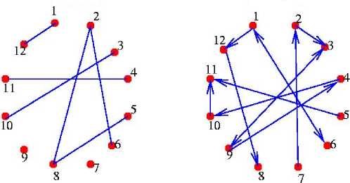
We present in [Fig. 12] an example of the kind of structures which can be obtained: we compare in particular an RG and a DRG of equal small size $N=12$, with the same $p\sim 1/N$ (hence $z\sim 1$) value. This figure makes evident the completely different topology with respect to the brain chain, where for the same connectivity value $n=1$ one would find a single connected component with directed links $i\rightarrow i+1$ (see [Fig. 1]). Instead, in the shown example, looking at the case of the undirected random graph for simplicity, we observe two isolated nodes, three connected component of size 2, and one connected component of size 4.

The figure also makes evident that in the directed case [42, 43, 44, 45], since the existence of a path connecting $i$ to $j$ does not usually imply the existence of a path connecting $j$ to $i$, for each given node one can define:

• the out-component, which is the set of all nodes that can be reached from it;

• the in-component, which is the set of all nodes from which it can be reached;

• the strongly connected component, which is the set of all the nodes that can be reached from it $and$ from which it can be reached, hence the intersection of the in-component and the out-component;

• the weakly connected component, which is the set of all the nodes that can be reached from it $or$ from which it can be reached, hence the union of the in-component and the out-component; this corresponds to the connected component of the node in the graph obtained by disregarding the directionality.

Figure 13: A sketch of the bow tie topology structure characteristic of directed network [44]: with respect to the notation used in the text, the two bows correspond to the giant components ${\cal I}\setminus{\cal S}_{sc}$ and ${\cal O}\setminus{\cal S}_{sc}$ respectively, whereas the tie represents the giant strongly connected component ${\cal S}_{sc}={\cal I}\cap{\cal O}$. Here we consider the most general case in which ${\cal W}={\cal I}\cup{\cal O}\cup{\cal T}$, where ${\cal T}$ contains in particular the paths linking the two bows without passing across the tie, which have been observed in real network such as the web [45].

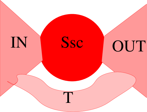
The analogous of the “phase transition” in an undirected random graph can now be characterized by the possible formation: of a giant in-component ${\cal I}$, containing $I=s_{I}N$ nodes; of a giant out-component, ${\cal O}$, containing $O=s_{O}N$ nodes; of a giant strongly connected component, ${\cal S}_{sc}={\cal I}\cap{\cal O}$, containing $S_{sc}=s_{sc}N$ nodes; of a giant weakly connected component ${\cal W}$, containing $W=s_{w}N$ nodes. In fact, one usually expects to observe two different transitions, i.e. two different abrupt changes in the properties of the system in the large $N$ limit: at the lower average in/out-degree $z^{w}_{c}$, corresponding to the critical average degree in the undirected graph, where it appears the giant weakly connected component, and at the higher average in/out-degree $z^{d}_{c}$, which gives the effective transition in the directed network, where the other giant components appear contemporaneously.

For $z\geq z^{d}_{c}$ the resulting picture is captured by the bow tie structure sketched in [Fig. 13], which has been observed in many different real networks [45, 46]: notice that the appearance of the giant in-component (respectively out-component) corresponds to the divergence of the number of nodes which can be reached from a given one (respectively from which a given one can be reached), i.e. a node is in the giant in-component if its out-component diverges, and vice-versa. Moreover, above the transition, it can be necessary to introduce one more giant component in order to fully characterize the topology, since one can have ${\cal W}\supset({\cal I}\cup{\cal O})$: this is in particular the case when there are directed paths between ${\cal I}$ and ${\cal O}$ which do not pass across the strongly connected component ${\cal S}_{sc}$, as it has been found in the structure of the web [45], which can be seen as a directed graph characterized by power law in/out-degree distributions.

The formalism of the probability generating functions for directed random graphs [43, 44] turns out to be particularly simple when the in/out-degree distribution factorizes, ${\cal P}_{k_{in},k_{out}}={\cal P}_{k_{in}}{\cal P}_{k_{out}}$, since the in and out components are independent in the large network size $N$ limit, so that one has simply $s_{sc}=s_{I}s_{O}$. For the considered case of ${\cal P}(k_{in})={\cal P}(k_{out})$ given by Eq. (36), the transition does still occur at the critical average in/out-degree $z^{d}_{c}=1$, and the giant in-component and out-component have the same size:

$$s_{I}=s_{O}=1-v(z),$$ (41)

where $v(z)$ is once more given by the solution of Eq. (40). Then, $s_{sc}=(1-v(z))^{2}$, whereas the fraction of nodes in ${\cal I}\setminus{\cal S}_{sc}$, and equivalently in ${\cal O}\setminus{\cal S}_{sc}$, is equal to $v(z)(1-v(z))$: the three regions in the bow tie have roughly the same size in the thermodynamic limit, as it has been observed in real networks [45], for $v\sim 1/2$, hence $z\sim\log 4$. Moreover, one simply has $z^{w}_{c}=z^{d}_{c}/2$: since when $v(z)$ is solution of Eq. (40) one has $v(2z)=v^{2}(z)$, it follows that, in the region $z>z^{d}_{c}$, $s_{w}=1-v^{2}(z)=s_{I}+s_{O}-s_{sc}$, which confirms that here ${\cal W}={\cal I}\cup{\cal O}$.

Figure 14: The local tree-like structure characteristic of Erdős-Rényi random graphs: on the left we consider the damage spreading on a directed random graph $D(N,p)$, with $z=\langle k_{out}\rangle=\langle k_{in}\rangle=3$, and on the right the one in the undirected network with the same $p$ value, $G(N,p)$.

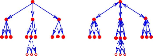
The other key ingredient of the topology of Erdős-Rényi random graph is that their structure, for not too large $p$-values, is tree-like: this is rigorously correct for the finite size connected components, both below and above the critical point, since it can be shown that here the probability of closed loops approaches zero in the limit $N\rightarrow\infty$, but it is locally valid also within the giant connected components, where the closed loops can be neglected in a first approximation. We compare in [Fig. 14] these kind of structures for a DRG and for an RG with the same $z=3$ value: notice that in the first case one has $z_{2}=\langle k_{in}\rangle\langle k_{out}\rangle=z^{2}$, where in the second case one gets the same results, $z_{2}=z^{2}$, from Eq. (38). In other words, in random directed network the probability to have both the link $i\rightarrow j$ and the link $j\rightarrow i$ is $\sim p^{2}$, and it is therefore negligible in the region $p\ll 1$ that we are studying, whereas in undirected random graphs we have to consider the edges emerging from the node apart the one along which the signal arrived, in order to make a meaningful computation.

As we are going to discuss, this difference is evident in the results on the damage spreading at short time in the BDE models on random graphs, that can be predicted quite accurately on the basis of the local tree-like topology. Moreover, when considering randomly distributed delays, though also here two paths with the same space length along the network do not usually have the same time length, because of the local tree-like topology, the number of different concurrent paths connecting two given nodes does not increase as fast with the average in/out-degree as in the previously considered deterministic braid chain.

Finally, we note that on the behavior of $D(N,p)$ there are detailed rigorous mathematical results [33] (see also [34] and references therein), which would require a definitely deeper analysis for being summarized.

4.2 The free models with equal delays

We introduce the free models, defined by Eq. (1), with all the delays equal to the same time unit $\tau_{0}=1$ day, on the directed random graph, $D(N,p)$, and we study as usual the consequences of a damage initially destroying a single firm for a duration $\tau_{c}$. For simplicity, we limit the analysis to the case $\tau_{c}=\tau_{0}$.

In the presence of stochasticity in the network structure, the BDE system (3) can no more be reduced, and one has in principle to solve a set of $N$ equations in $N$ variables, which can be rewritten in the form:

$$x_{i}(t)=\mu_{i}(t)\prod_{j\in{\cal I}(i)}x_{j}(t-\tau_{0})\hskip 21.68121pti=1,...,N.$$ (42)

Here the product, which means as before the AND Boolean operators $\wedge$, runs over all the values of the index $j$ labeling firms which are suppliers of $i$, hence belonging to the set of nodes ${\cal I}(i)=\{j:A_{ij}\neq 0\}$, which corresponds to the definition of the node in-component ${\cal I}(i)$; the in-degree of the node is the total number of suppliers of firm $i$, i.e. $I(i)=k_{in}(i)$. Analogously, the out-component of the node, ${\cal O}(i)=\{j:A_{ji}\neq 0\}$, corresponds to the firms which are customers of $i$, which total number is $k_{out}(i)$.

Therefore, Eq. (42) makes evident that the properties of the BDE system strongly depend on the probability distributions of the in/out-degree, which in the considered case are independent, and described by Eq. (36), with mean values $\langle k_{in}(i)\rangle=\langle k_{out}(i)\rangle=(N-1)p=z$. Hence, for increasing $z$ values, the properties of the solutions will reflect the appearance of giant in/out-connected components in the graph, and one will find different kinds of solution for average in/out-degree lower or higher than the critical value $z^{d}_{c}=z_{c}=1$.

In detail, the damage spreading in this simple BDE model can be understood with the same argument used for evaluating the average size of the connected components in the graph: at $t=1$, the signal propagates from the node $i$, occupied by the initially damaged firm, to its first neighbors, which average number is $z_{1}=z$; at $t=2$, it reaches the second neighbors, which average number is $z_{2}=z^{2}$, and so on. From Eq. (38) it follows that at time $t$ the damage did spread up to reach in average $z^{t}$ nodes, hence:

$$\langle\theta_{tot}(t)\rangle\simeq z^{t}\mbox{ for }t\ll\log N/\log z,\hskip 36.135pt\mbox{ (DRG)}.$$ (43)

This implies that the average number of firms which production is impaired increases with time only if $z>z^{d}_{c}=1$, i.e. only if the graph is above its transition point.

The argument does make use of the local tree-like structure, since we are implicitly assuming that the probability for two node reached at a given time step of being themselves connected by a different path, i.e. the probability of closed loops, can be neglected. In fact, this argument breaks down roughly at the time where the signal propagated to the whole connected component to which the initial node $i$ belongs, and one can find different situations:

• $i$ is in a connected component containing a small number of nodes, $S_{c}=0(1)$; in this case one expects that there are no loops, hence the system can completely recover from the initial damage, i.e. $\theta_{tot}(t)=0$ in the large time limit; a randomly chosen initial node $i$ will belong almost surely to a connected component containing a finite number of nodes, in the $N\rightarrow\infty$ limit, for $z<z^{d}_{c}$, and with probability $v(z)$ for $z>z^{d}_{c}$;

• the graph is above the critical point and $i$ belong to a giant connected component; because of the presence of closed loops, here a finite fraction of the firms will be impaired in the asymptotic solution, and the economic network does never recover completely from the initial destruction event.

Such results can be explained by noticing that, in our model, there are firms which have no “clients” in the network. This surprising possibility simply arises from the fact that some firms have only final customers as clients, not other firms. For these “final-demand” firms, being unable to produce does not have any consequences on the rest of the productive system, only on household well-being. Since $z$ measures the average number of clients which are in the network, in the limit of a large total number $N$ of firms, the phase-transition just corresponds to the fact that, for $z<1$, the most of the firms are in this peculiar situation, or have a few customer firms which are themselves in this peculiar situation, and so on, so that the initial damage usually does not propagate; conversely, as soon as $z$ is larger than one, a finite fraction $1-v(z)$ of the firms have clients in the network, which have themselves other clients in the network, and so on.

To make more quantitative the analysis, in the large $N$ limit, one can say that in directed random network above the transition point, in order to observe damage spreading up to reach a finite fraction of the network, the initially attained firm has to belong to the giant in-component, $i\in{\cal I}$: this occurs with probability $1-v(z)$. Moreover, in the same limit, one expects that finally all the firms in the giant out-component ${\cal O}$ will be impaired, which means a fraction $s_{O}=1-v(z)$ of the whole network. Correspondingly, we find:

$$\langle\theta_{tot}(t)\rangle\simeq\left\{\begin{array}[]{lcl}z^{t}&\mbox{ for }&t\ll t_{trans}\\ \left[1-v(z)\right]^{2}N&\mbox{ for }&t\gg t_{trans},\>N\gg 1\\ \end{array}\right.$$ (44)

where the time that $\langle\theta_{tot}(t)\rangle$ takes before reaching the asymptotic constant average value is quite short also for large $N$ values, since it is of order $t_{trans}\sim\log([1-v(z)]N)/\log z$.

Interestingly, $[1-v(z)]^{2}$ is also the fraction of nodes which are in the giant strongly connected component, ${\cal S}_{sc}$, of the network; nevertheless, one should note the different meaning of the two quantities: when the initial node belongs to ${\cal I}$, the total number of firms which activity is finally impaired is $[1-v(z)]N=S_{O}$, definitely larger than $S_{sc}$ for small $v(z)$ values. This point can be better understood by looking at the Erdős Rényi undirected random graphs with the same average degree $z>1$: here, the initially damaged firm $i$ has to belong to the giant connected component ${\cal S}_{gc}$, and the firms which activity is finally impaired are the ones in ${\cal S}_{gc}$ as well, hence we find again that $\langle\theta_{tot}(t)\rangle$ approaches $[1-v(z)]^{2}N$ at large times, though it is clearly $S_{sc}=1-v(z)$.

Summarizing, both in the DRG and in the RG, the average asymptotic density of fully active firms, when the networks is above the transition point, turns out to be:

$$\langle\rho_{asym}(z)\rangle=1-[1-v(z)]^{2}=2v(z)-v^{2}(z),$$ (45)

where we recall that $v(z)$ is the solution of Eq, (40)). Instead, one important difference between the behavior of the considered free BDE systems with equal delays on directed and undirected random graphs concerns the short time dynamics: as it is shown in [Fig. 14], in the undirected case the signal does also propagate back to the node from which it is arrived and, correspondingly, to correctly describe the behavior of $\langle\theta_{tot}(t)\rangle$, Eq. (43) should be replaced by:

$$\langle\theta_{tot}(t)\rangle=\sum_{l=0}^{[t/2]}z^{t-2l}\mbox{ for }t\ll\log N/\log z,\hskip 36.135pt\mbox{(RG)},$$ (46)

where as usual we denote $[y]$ the largest integer smaller than $y$.

Figure 15: Data on free models on random graphs with a large number of nodes $N\gg 1$ and deterministically chosen delays all equal to $\tau_{0}=1$ day. The obtained results are averaged over at least ${\cal N}_{s}=200$ different configurations of the links. On the left, we present the short time behavior of the average total number of impaired firms, $\langle\theta_{tot}(t)\rangle$, both in the directed random graph, $D(N,p)$, with average in/out-degree $z\simeq Np=1.5$ and in the undirected Erdős-Rényi one, $G(N,p)$, with the same $p$ value; here $N=5000$. On the right, we plot $\langle\theta_{tot}(t)\rangle$ in the directed random graph, $D(N,p)$, for different $z\simeq pN$ values above the transition point and $N=10000$. The obtained curves are compared with the corresponding expected behaviors, given by Eq. (43) for DRGs, and by an approximation of Eq. (46) for RGs, respectively (see the text for details).

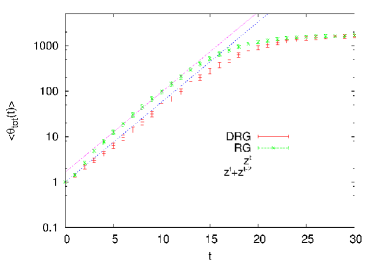
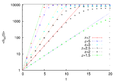
We present in [Fig. 15] the results of numerical simulations of the BDE free model with equal delays on random graphs with a large number of nodes $N=5000\div 10000$, for different values of $z>1$, above the transition point. On the left, we compare the short time behavior of $\langle\theta_{tot}(t)\rangle$ in a directed random graph, and in an undirected one with the same $z=1.5$ average degree. Here, the regime preceding the attainment of the asymptotic constant value is relatively long, and one can appreciate the difference between the DRG case, described by Eq. (43), hence $\langle\theta_{tot}(t)\rangle\simeq z^{t}$, and the RG one, where at not too short times the data are better in agreement with $\langle\theta_{tot}(t)\rangle\simeq z^{t}+z^{t-2}$, which is an approximation of Eq. (46). Notice moreover that one gets compatible asymptotic values in both of the cases. On the right we plot $\langle\theta_{tot}(t)\rangle$, as a function of $t$, in directed random graphs with different $z>1$ values, by comparing the curves with the expected $z^{t}$ short time behaviors. This figure makes also evident that the asymptotic total number of impaired firms is an increasing function of the average in/out-degree; moreover, already for $z$ as small as $z=5$, it practically coincides with the system size $N$, and the damage spreads in a few steps, $t_{trans}\sim\log N/\log z$, to all the firms.

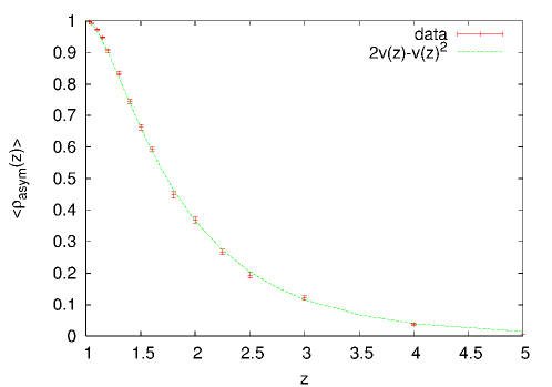
The results on the average asymptotic density, $\langle\rho_{asym}(z)\rangle$, as a function of the average in/out-degree $z$, are presented in [Fig. 16], and they turn out to be in very good agreement with the expected curve (see Eq.(45)), obtained by evaluating numerically the solution $v(z)$ of Eq. (40). The data shown in the figure correspond to the case of directed random graphs, but we checked that in undirected structures with the same average degree one gets definitely compatible results. This agreement does also imply that for the considered number of nodes, $N=10000$, the corrections to the behavior in the limit $N\rightarrow\infty$ of $\langle\rho_{asym}(z)\rangle$ are practically negligible.

Figure 16: Data on free models on directed random graphs, with large network size, $N=10000$, and deterministically chosen delays all equal to $\tau_{0}=1$ day. Here the results are averaged over at least ${\cal N}_{s}=200$ different configurations of the links. We plot the asymptotic average density, $\langle\rho_{asym}(z)\rangle=\lim_{t\rightarrow\infty}\langle\rho(t)\rangle$, as a function of the mean in/out-degree $z$, compared with the expected behavior, given by Eq. (45).

To conclude this section, the present results suggest that the study of these simple BDE systems on more complex random structures could prove useful also for better understanding the topology of the networks themselves, and in particular for evaluating the size of their connected components, which is difficult to be analytically computed in the case of realistic directed networks, where the probability distributions of the out and in degree do not factorize [47]. A first step in this direction would be to consider (directed) “small-world” networks [39], which in some sense interpolate between the topology of the braid chain and the one of the Erdős-Rény random graph.

It is moreover important to stress that the discussed damage spreading in free BDE models is not to be confused with other well known examples of damage spreading, such as in particular the spreading of epidemic diseases or of the effects of node deletions [40, 41]. In fact, on the one hand, here we have assumed that the damage propagates to all the nodes in the out-component of the concerned one, though with possibly different delays, and, on the other hand, a node attained by the consequences of the initial damage is not to be considered removed from the network, since it can recover.

4.3 The free models with random delays

We now turn onto the study of the free BDE model on a directed random graph, when the delays are randomly chosen according to Eq. (4). The system is described by a set of equations analogous to Eq. (42):

$$x_{i}(t)=\mu_{i}(t)\prod_{j\in{\cal I}(i)}x_{j}(t-\tau_{i,j}),\hskip 21.68121pti=1,...,N.$$ (47)

where the $\{\tau_{i,j}\}$ variables are independently uniformly distributed in the interval $[\tau_{min},\tau_{max}]$. Hence the time is in units of $\tau_{min}=1$ day, and we will take as usual $\tau_{max}=10$ days, limiting moreover the analysis to the case in which the duration of the initial damage is $\tau_{c}=\tau_{min}$.

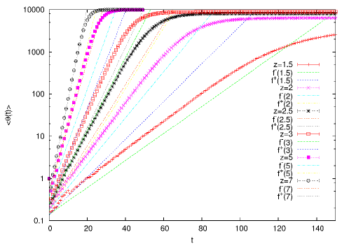
In order to understand the dynamics, we start by noticing that in the first time step the signal propagates in average to $z/\tau_{max}$ other firms. In the next time steps, one still expects to observe an exponential damage spreading, for networks above the transition point $z^{d}_{c}=1$. Moreover, the structure is locally tree-like: this means that, at enough short times, the signal propagates along each given branch (and sub-branch and so on) of the tree independently; correspondingly, since the propagation paths of different time lengths are not concurrent, one expects that the random delays will turn out first of all in a global rescaling of the time of a factor $1/\tau_{av}$, where $\tau_{av}=\langle\tau_{i,j}\rangle$.

Figure 17: The total number of impaired firms, $\theta_{tot}(t)$, as a function of time, in the free model on a directed random graph with a large network size $N=10000$ and different $z$ values. The data are averaged over at least ${\cal N}_{s}=200$ different configurations both of the links and of the random delays, the last being chosen uniformly distributed between $\tau_{min}=1$ day and $\tau_{max}=10$ days. We compare the curves for each $z$ value with the expected short time lower limit $f^{-}(z,t)=f(z^{-}_{eff},t)$ and upper limit $f^{+}(z,t)=f(z^{+}_{eff},t)$, where $f$ is given in Eq. (52). See the text for details.

One obtains:

$$\langle\theta_{tot}(t)\rangle=\frac{z}{\tau_{max}}z_{eff}^{t/\tau_{av}}\mbox{ for }t\ll\log N/\log z_{eff}.$$ (48)

The effective average in/out-degree which appears into this law has to approach $z$ when $z\rightarrow 1^{+}$, hence

$$z_{eff}\geq z^{-}_{eff}=z.$$ (49)

Nevertheless, since the signal from a given node propagates to its customers up to the time $t+\tau_{max}$, one also finds an effective increasing of the average in/out-degree, which can be easily overestimated:

$$z_{eff}\leq z^{+}_{eff}=z\sum_{l=0}^{\infty}\left(\frac{z}{\tau_{max}}\right)^{l}=\frac{z}{1-z/\tau_{max}}.$$ (50)

Summarizing, at short times, for $z>1$, we get:

$$f^{-}(z,t)=f(z_{eff}^{-},t)\leq\langle\theta_{tot}(t)\rangle\leq f(z_{eff}^{+},t)=f^{+}(z,t),$$ (51)

where

$$f(z_{eff},t)=\frac{z}{\tau_{max}}z_{eff}^{t/\tau_{av}}.$$ (52)

We compare in [Fig. 17] the data on $\langle\theta_{tot}(t)\rangle$, for different values of the average in/out-degree $z>1$, and a large system size $N=10000$, with the expected upper and lower limits on the short time behaviors, given by Eq. (51). The curves do always lie between $f^{-}(z,t)$ and $f^{+}(z,t)$ in a large time window; they approach $f^{-}(z,t)$ for $z\rightarrow 1^{+}$, and $f^{+}(z)$ for large $z\gg 1$; in detail, the data at short times nearly coincide with $f^{+}(z,t)$ already for $z=3$.

Figure 18: The density of fully active firms $\rho(t)$ as a function of time in the free model on a directed random graph with different average connectivities $z>1$. Here we consider single typical configurations of the links. We compare the results for delays deterministically taken all equal to $\tau_{0}=1$ day with the ones for a single typical configuration of random delays, chosen uniformly distributed between $\tau_{min}=1$ day and $\tau_{max}=10$ days. We notice that the densities approach exactly the same values in the two cases.

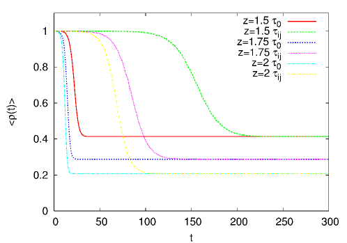
In the large time limit, since in the giant strongly connected component ${\cal S}_{gc}$ there are loops, one expects that at the end the damage will spread to the whole giant out-component ${\cal O}$, with the same probability $1-v(z)$ that in the model with deterministic delays. Correspondingly, we verified numerically that one still observes, for large $N$ values, an asymptotic average density of fully active firms $\langle\rho_{asym}\rangle=2v(z)-v^{2}(z)$, in agreement with Eq. (45). Moreover, for not too small $N$ values, one usually gets the same $\rho_{asym}$ for a given network configuration both for deterministic equal delays and for randomly chosen $\tau_{i,j}$ (see [Fig. 18]). This can be qualitatively understood because, if the initially attained firm is in a connected component where there are no loops, the economy can recover completely in both of the cases, whereas if it is in the giant in-component then the damage spreads to the whole out-component of the particular considered network.

Figure 19: The density of fully active firms $\rho(t)$ as a function of time in a given, quite peculiar, random directed network configuration with $z=0.525$ and $N=100$, after a perturbation of node $i=1$ of duration $\tau_{c}=1$ day. We compare results for deterministically chosen delays, all equal to $\tau_{0}=1$ day (lower curves), to the ones for a typical configuration of random delays, uniformly distributed between $\tau_{min}=1$ day and $\tau_{max}=10$ day (upper curves): notice that the asymptotic solutions display the same behavior of the density, which oscillates around a value definitely smaller than one, though the network is well below the crossover point $z\sim 1$. See the text for details.

Nevertheless, the asymptotic solutions of the considered free BDE systems, for the same directed graph configuration, do not need to be coincident when considering equal or random delays. This effect becomes evident for relatively small $N$, near or below the crossover point, hence for $z\lesssim 1$, since it is related to the presence of loops in connected components which contain an enough large fraction of the nodes, but are not the giant ones. More in detail:

• when the initially attained firm belongs to a component where there are no loops, the asymptotic solutions is given by $x_{i}\equiv 1\>\forall i$ in both of the cases;

• when it belongs to the giant in-component, hence containing an enough large number of loops, the asymptotic solutions is given by $x_{i}\equiv 0\>\forall i\in{\cal O}$, and $x_{i}\equiv 1\>\forall i\in{\cal W}\setminus{\cal O}$, hence the solutions are again the same in both of the cases, apart possibly for a small fraction of nodes which approaches zero in the limit $N\rightarrow\infty$;

• in intermediate situations, one usually finds periodic solutions which can be largely different.

Figure 20: The density of fully active firms $\rho(t)$ as a function of time, after a perturbation of node $i=1$ of duration $\tau_{c}=1$ day, in some quite peculiar random network configurations with $z=0.525$, which probability is not negligible already for the relatively large size $N=100$ that we considered. In all of the cases, we compare results for deterministically chosen equal delays (lower curve) with the ones for a typical configuration of random unequal delays (upper curve), as in the previous figure. Notice that here the densities approach definitely different asymptotic behaviors in the two cases. See the text for details.

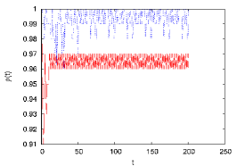
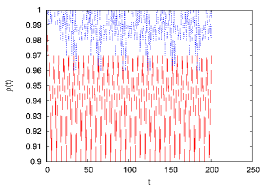
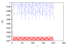
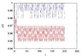
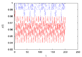
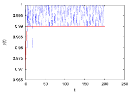
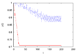
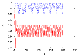
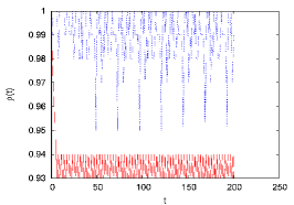
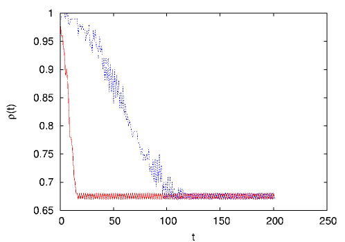
Though a detailed analysis of the finite $N$ behavior of free BDE models on directed random graphs is beyond the scope of the present paper, we show in [Fig. 19] and [Fig. 20] some examples of peculiar configurations of $D(N,p)$, with $N=100$ and $z=0.525$, well below the crossover point.

We note that the observed behavior does also depend on the position of the firm which is initially destroyed, here taken to be $i=1$ in all of the cases. We compare the data on the density of fully active firms $\rho(t)$ for deterministically chosen delays all equal to $\tau_{0}=1$ day with the ones for a typical configuration of random unequal delays, uniformly distributed between $\tau_{min}=1$ day and $\tau_{max}=10$ days; the duration of the initial damage is $\tau_{c}=1$ day in both of the cases. The results confirm that one can observe different asymptotic average densities, which implies largely different periodical solutions of the system; moreover, the probability of these disordered network configurations is not negligible, since we have observed not compatible $\rho_{asym}$ values in $\sim 1/10$ of the considered samples.

4.4 The forced models

We conclude this work by presenting some preliminary results on the forced models, as defined by Eq. (2), on a directed random graphs structure $D(N,p)$. The equation for the variable $x_{i}$ of the system (3) can be written as:

$$x_{i}(t)=\mu_{i}(t)\overline{x}_{i}(t-\tau_{0})\vee\prod_{j\in{\cal I}(i)}x_{j}(t-\tau_{0})\hskip 21.68121pti=1,...,N.$$ (53)

when the delays are deterministically taken all equal to $\tau_{0}=1$ day, and:

$$x_{i}(t)=\mu_{i}(t)\prod_{j\in{\cal I}(i)}[\overline{x}_{i}(t-\tau_{i,j})\vee x_{j}(t-\tau_{i,j})]\hskip 21.68121pti=1,...,N.$$ (54)

for random delays. We study, as usual, the damage spreading after the initial destruction of a single firm, that we take for simplicity of duration $\tau_{c}=1$ day.

As soon as the initial attained firm belongs to a component where there are no loops, the economy will recover completely as in the previously considered free models, hence the asymptotic solution is $x_{i}\equiv 1\>\forall i$. For large $N$, this happens in particular almost surely below the critical point of the directed random graph $z_{c}^{d}=1$, and with probability $v(z)$ for $z>z_{c}^{d}$, where $v(z)$ is the solution of Eq. (40).

Figure 21: The density of fully active firms $\rho(t)$ as a function of time, after an initial perturbation of node $i=1$ of duration $\tau_{c}=1$ day, in the forced model on a directed random graph with a large network size $N=10000$ and average input/output degree $z=7\gg z^{d}_{c}$. Here we consider a single (typical) configuration of the links, and we compare the results for the case of delays taken all equal to $\tau_{0}=1$ day with the ones for a typical configuration of random unequal delays, chosen uniformly distributed between $\tau_{min}=1$ day and $\tau_{max}=10$ days.

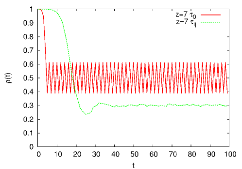
Nevertheless, because of the external rescue inputs, one expects that also in the region $z\gg z_{c}^{d}$, though the damage spreads almost surely ($v(z)\ll 1$) to the whole giant connected out-component, whose size is approximately $N$ in this limit, the average fraction of fully active firms in the asymptotic solution is larger then zero, i.e. the economy can partially recover. More in detail, for deterministically taken equal delays, since each firm recovers both if all of its suppliers did recover and if its activity has been already impaired for a duration $\tau_{0}$, one expects that, in the asymptotic solution, in average the firm is fully active one half of the time. This means $\langle\rho_{asym}\rangle=1-[1-v(z)]^{2}/2\sim 1/2$, for $z\gg 1$. In the presence of random delays, since there is a larger number of concurrent paths of different time lengths, and the activity of a given firm can be impaired for a different duration of time depending on the good which is lacking, the asymptotic average density is expected to be smaller.

We present in [Fig. 21] our numerical results on the behavior of $\rho(t)$, as a function of time, for a single, typical, configuration of the directed random graph, of large size $N=10000$, and average in/out-degree $z=7\gg z_{c}^{d}$. In fact, for deterministically chosen equal delays the asymptotic density oscillates around the average value $1/2$, whereas for random delays it takes the lower average value $\rho_{asym}\simeq 0.3$. Moreover, in the first case the oscillations of the density are quite strong, with lower value $\simeq 0.4$ and upper value $\simeq 0.6$; hence a finite fraction of the firms, of order $0.2N\simeq 2000$, is involved into them.

Figure 22: A qualitative sketch of the expected behavior of the probability distribution of impaired firms as a function of the distance of their position from the center of the connected component of the graph. See the text for details.

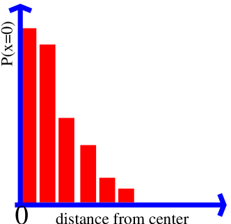
One can explain qualitatively this result by arguing that the damage starts to spread from some firm in the periphery of the connected component of the graph, rapidly propagating into the center. Then, because of the external inputs, the most of the economy recovers, apart from a few firms which are once again in the periphery, and have been reached later by the wave of damage: these will be responsible for the forthcoming impulse. Roughly speaking, the nodes with larger in/out-degree are the ones occupying the more central positions, whereas a small in-degree means that the node is more unlikely reached by the damage propagation and a small out-degree means that it is more unlikely to transmit the damage, so that these nodes are to be considered in the periphery in both of the cases. This picture is sketched in [Fig. 22], and it is quite intriguing, since it implies that there is a large factor of unpredictability in the behavior of the solution of the BDE system. A first step towards a more quantitative analysis could be to look at the modular structure of the directed random graph [48]. Notice however that the random delays have the effect of smoothening this oscillating behavior.

5 Conclusions

We have studied the propagation of an initial damage, which destroys a single firm for a given time, in production networks. In the considered free models, which represent isolated networks, since the local firm dynamics is controlled by a logical AND function of the inputs, the damage can invade a finite fraction of the nodes or the whole network when these two conditions are fulfilled: i) the nodes mean input connectivity is larger than one; ii) the duration of the initial damage is larger than the smallest propagation time between two nodes. In particular, for a braid chain (deterministic and connected) topology, these conditions mean that in the asymptotic solution the production of all the firms is impaired.

Damage spreading velocity strongly depends upon network topology: we have shown that the number of attained firms increases linearly with time for the braid chain and exponentially for the directed random graphs. We have also introduced a distribution of delays, and we have found that the propagation velocity is dominated by the fastest segments (the smallest delay) in the braid chain, while the average delay limits speed on the directed random graph. Moreover, in random networks the saturation level of the fraction of impaired firms does not depend upon the distribution of delays, but only upon the particular network topology through the size of the connected component, which is in average not negligible as soon as the mean in/out-degree is larger than one.

External supplies, modeled here in terms of forced networks, limit damage and the asymptotic solutions are periodic: waves of damage move across the structure. In the considered forced models with distribution of delays, the transient before that these solutions are reached diverges exponentially with the network size, though the average density of fully active firms approaches a nearly constant value after a definitely shorter effective transient. This effective transient corresponds approximately to the duration of the first cycle of propagation of the damage across the connected component of the networks, which happens similarly to that in the free models, with linear or exponential speed depending on the topology. Finally, periodic dynamics are obtained also when the duration of the initial damage is smaller than the smallest propagation time between two nearest neighbor nodes.

The models that we have used are extremely simplified with respect to real production networks, and firms behavior is represented in a very idealized way. Still, results from this simple analysis suggest that:

• Damage spreads in absence of sufficient stocks and flexibility; as a result, production shortages are extended and can survive for periods much longer than the duration of the initial local damage. This result suggests that an affected economy can suffer from disaster consequences even after all physical damages have been repaired.

• The presence of multiple concurrent production paths with different time lengths does not necessarily imply a slowing down of the speed of the signal, which can propagate as fast as the shortest path, depending on the topology. This result suggests that the most vulnerable supply chains control the macroeconomic losses and that vulnerability analysis should focus on the identification of key vulnerabilities.

Appendix A

The average total number of impaired firms $\langle\theta_{tot}(t)\rangle$, in the free model on a braid chain network with $n=1$, defined accordingly to Eq. (8) and Eq. (6), can be expressed as function of the probability ${\cal P}({\cal T}_{k},k)$, where ${\cal T}_{k}$ is the sum of $k$ random variables $\tau_{i,j}$:

$$\langle\theta_{tot}(t)\rangle \equiv \langle\sum_{i=1}^{N}\overline{x}_{i}(t)\rangle\equiv\sum_{i=1}^{N}\int\prod d\tau{\cal P}(\tau)\overline{x}_{i-k}(t-{\cal T}_{k})=$$ (55)

$$= \sum_{k=[t/\tau_{max}]+1}^{[t]\tau_{max}}{\cal P}([t],k)\sum_{i=1}^{N}\delta_{i-k,1}=\sum_{k=[t/\tau_{max}]+1}^{[t]\tau_{max}}{\cal P}([t],k).$$

Here $[v]$ means the integer part of $v$, and we are assuming for simplicity that the duration of the initial damage is $\tau_{c}=\tau_{min}=1$ day, hence we are using the conditions on the initial state of the system, $\{x_{i}(t)=\delta_{i,1}(0)\}$ for $t\in[0,1]$.

One has, from Eq. (4):

$$\langle\tau_{i,j}\rangle = \int_{1}^{\tau_{max}}d\tau_{i,j}{\cal P}(\tau_{i,j})\tau_{i,j}=\frac{(\tau_{max}+1)}{2}$$ (56)

$$\sigma^{2}_{\tau_{i,j}} = \frac{(\tau_{max}+1)(2\tau_{max}+1)}{6}-\frac{(\tau_{max}+1)^{2}}{4},$$ (57)

for the mean value and the variance of the distribution of the delays, respectively. For $k\geq 2$, assuming that the variables are independent (which is clearly an approximation for $k>N$), one can apply the central limit theorem:

$${\cal P}({\cal T}_{k},k)\simeq{\cal P}_{G}(T_{k},k)=\frac{1}{\sqrt{2\pi k\sigma^{2}_{\tau_{i,j}}}}\exp\left(-\frac{({\cal T}_{k}-k\langle\tau_{i,j}\rangle)^{2}}{2k\sigma^{2}_{\tau_{i,j}}}\right).$$ (58)

By using this approach, we find:

$$\langle\theta_{tot}(t)\rangle\simeq\left\{\begin{array}[]{ll}1&t\in[0,1)\\ {\cal P}(1,1)={1}/{\tau_{max}}&t\in[1,2)\\ {1}/{\tau_{max}}+\sum_{k=2}^{([t]\tau_{max})}{\cal P}_{G}([t],k)&t\in[[t],[t]+1),\>2\leq t\leq\tau_{max}\\ \sum_{k=[t/\tau_{max}]+1}^{([t]\tau_{max})}{\cal P}_{G}([t],k)&t\in[[t],[t]+1),\>t>\tau_{max}\end{array}\right.$$ (59)

where the sums are clearly dominated by the terms corresponding to $k^{*}\langle\tau_{i,j}\rangle\simeq[t]$, i.e. the same that are best approximated by the Gaussian distribution. The corresponding average density can be straightaway obtained from Eq. (9).

In the large $t$ limit, $\langle\theta_{tot}(t)\rangle$ approaches quite rapidly a nearly constant value, that in the numerically studied case of $\tau_{max}=10$ is found to be:

$$\lim_{t\rightarrow\infty}\langle\theta_{tot}(t)\rangle\simeq\lim_{t\rightarrow\infty}\sum_{k=[[t]/\tau_{max}]+1}^{[t]\tau_{max}}{\cal P}_{G}([t],k)\simeq 0.182,$$ (60)

which gives, again from Eq. (9):

$$\lim_{t\rightarrow\infty}\langle\rho(t)\rangle=1-\frac{0.182}{N}.$$ (61)

Appendix B

By using the Boolean rule $\overline{a\wedge b}=\overline{a}\vee\overline{b}$, Eq. (13), defining the free model on the circulant matrix, turns out to be equivalent to:

$$\overline{x}_{i}(t)=\sum_{j=1}^{n}\overline{x}_{i-j}(t-\tau_{i,i-j}),$$ (62)

which, in the case of equal delays $\{\tau_{i,j}=\tau_{0}\>\forall i,j\}$, allows the simplification:

$$\overline{x}_{i}(t) = \sum_{j_{1}=1}^{n}\sum_{j_{2}=1}^{n}\overline{x}_{i-j_{1}-j_{2}}(t-2\tau_{0})=$$ (63)

$$= \sum_{j_{1}=1}^{n}\sum_{j_{2}=1}^{n}\cdots\sum_{j_{k}=1}^{n}\overline{x}_{i-j_{1}-j_{2}-...-j_{k}}(t-k\tau_{0})=$$

$$= \sum_{j=k}^{kn}\overline{x}_{i-j}(t-k\tau_{0}),$$

since the different terms containing the same argument are redundant. Hence, by choosing $k=[t/\tau_{0}]=[t]$, one gets:

$$\theta_{tot}(t)=\sum_{i=1}^{N}\overline{x}_{i}(t)=\sum_{j=[t]}^{[t]n}\overline{x}_{i-j}(t-[t])=[t](n-1)+1\mbox{ for }t\in[[t],[t]+1),$$ (64)

where we are assuming $[t](n-1)+1\leq N$, and we used the conditions on the initial state of the system, $\{\overline{x}_{i-j}(t)=\delta_{i-j,1}\mbox{ for }t\in[0,\tau_{c})\}$, by considering for simplicity a duration of the initial damage $\tau_{c}=\tau_{0}$. This analysis confirms that, as soon as $n>1$, the system is dissipative, and in particular the total number of impaired firms (a constant function in each time step) is linearly increasing with time, with slope $n-1$. Correspondingly, for a finite size $N$, the asymptotically stable solution $\{x_{i}\equiv 0\>\forall i\}$, and the zero limit value of the density, are attained after the time $t_{trans}\simeq(N-1)/(n-1)$, in agreement with Eq. (19). One can moreover analogously show that, for $\tau_{c}\neq\tau_{0}$, the density is still linearly decreasing with time, and the asymptotic solution is the same for $\tau_{c}>\tau_{0}$, whereas it is periodic of period $\tau_{0}$ for $\tau_{c}<\tau_{0}$, as described in Section 3.4.

In order to work out the same approach for randomly distributed delays, we label $l_{h}=\sum_{v=1}^{h}j_{v}$. One finds:

$$\overline{x}_{i}(t) = \sum_{j_{1}=1}^{n}\sum_{j_{2}=1}^{n}\cdots\sum_{j_{k}=1}^{n}\overline{x}_{i-l_{k}}\left(t-\sum_{h=0}^{k}\tau_{i-l_{h},i-l_{h+1}}\right)=$$ (65)

$$= \sum_{j=k}^{kn}\sum_{\{l_{1},l_{2},\dots,l_{k}\}:l_{k}=j}\overline{x}_{i-j}\left(t-\sum_{h=0}^{k}\tau_{i-l_{h},i-l_{h+1}}\right).$$

Since the $\{\tau_{i,j}\}$ are independent identically distributed random variables which take integer values (in unities of $\tau_{min}$) in the interval $[1,\tau_{max}]$, it follows that their sums ${\cal T}_{k}=\sum_{h=0}^{k}\tau_{i-l_{h},i-l_{h+1}}$ take integer values in the interval $[k,k\tau_{max}]$ with probability ${\cal P}({\cal T}_{k},k)$; moreover, terms $\overline{x}_{i-j}$ with the same argument are redundant. The average over the disorder can be therefore computed as:

$$\langle\overline{x}_{i}(t)\rangle = \int\prod d\tau{\cal P}(\tau)\overline{x}_{i}(t)=$$ (66)

$$= \sum_{j=k}^{kn}\sum_{{\cal T}_{k}=k}^{k\tau_{max}}{\cal P}({\cal T}_{k},k)\overline{x}_{i-j}(t-{\cal T}_{k}).$$

Then, one can choose in particular $k$ values in the different terms such that $t-{\cal T}_{k}$ is always in the initial interval; in detail, looking for simplicity only at $t$ values which are integer multiple of $\tau_{max}$, one has:

$$\langle\overline{x}_{i}(t)\rangle = \left[\sum_{j=t}^{nt}{\cal P}_{t}(t,t)+\sum_{j=t-1}^{n(t-1)}{\cal P}_{t}(t,t-1)+...\right.$$

$$... + \left.\sum_{j=t/\tau_{max}}^{nt/\tau_{max}}{\cal P}_{t}(t,t/\tau_{max})\right]\overline{x}_{i-j}(0)=$$ (67)

$$= \sum_{j=t/\tau_{max}}^{t}\sum_{k=j}^{nj}{\cal P}_{t}(t,j)\delta_{i-j,1},$$

and therefore, up to the time $t_{trans}$ at which $\langle\theta_{tot}(t_{trans})\rangle\simeq N$, one has:

$$\langle\theta_{tot}(t)\rangle=\sum_{k=t/\tau_{max}}^{t}[(n-1)k+1]{\cal P}_{t}(t,k).$$ (68)

Here, ${\cal P}_{t}(t,k)$ is the probability for the signal to have propagated $k$ steps along the chain at time $t$, which can be approximated by a Gaussian with mean value $k\langle\tau_{i,j}\rangle$ and variance $k\sigma^{2}_{i,j}$ (see Eq. (58)), but needs to be correctly normalized in order to get:

$$\sum_{k=t/\tau_{max}}^{t}{\cal P}_{t}(t,k)=1\hskip 14.45377pt\forall t.$$ (69)

In detail, we take ${\cal P}_{t}(t,k)\simeq C(t){\cal P}_{G}(t,k)$, where the normalization constant $C(t)$ approaches rapidly its large time limit $C_{\infty}\simeq 1/0.182$, in agreement with Eq. (60).

In fact, we notice that one would get straightaway a linear behavior of $\langle\theta_{tot}(t)\rangle$ from Eq. (68), by taking ${\cal P}_{t}(t,k)\equiv 1$; nevertheless, the Gaussian approximation and the use of the correct normalization constant $C(t)$ are essential in order evaluate accurately enough the slope. These results therefore confirm, from a different point of view, the analysis of Section 3.5; in particular, for the considered case of $n=20$ and $\tau_{max}=10$, the density $\langle\rho(t)\rangle=1-\langle\theta_{tot}(t)\rangle/N$ obtained with this approach is in very good agreement with the numerical data, as shown in [Fig. 6].

Appendix C

Here we briefly recall the framework of probability generating functions [43, 44]: this allows to simply evaluate the size of connected components in Erdős-Rényi random graphs, and it is moreover well suitable to be generalized to directed networks and to more complex probability distribution ${\cal P}(k)$ of the node degrees.

One defines:

$${\cal G}_{0}(y)=\sum_{k=0}^{\infty}{\cal P}(k)y^{k},$$ (70)

which implies:

$${\cal P}(k)=\frac{1}{k!}\left.\frac{d^{k}}{dy^{k}}{\cal G}_{0}(y)\right|_{y=0}.$$ (71)

Analogously, the generating function for the probability distribution ${\cal P}_{1}(k)$, to have $k$ edges leaving a node apart the one from which the signal arrived, is given by:

$${\cal G}_{1}(y)=\sum_{k=0}^{\infty}{\cal P}_{1}(k)y^{k}=\frac{\sum_{k=0}^{\infty}(k+1){\cal P}(k+1)y^{k}}{\sum_{k=0}^{\infty}k{\cal P}(k)}=\frac{{\cal G^{\prime}}_{0}(y)}{z},$$ (72)

and in the Erdős Renyi random graph one has:

$${\cal G}_{0}(y)={\cal G}_{1}(y)=e^{z(y-1)}.$$ (73)

One can show in particular that, if ${\cal G}$ is the generating function for the probability of some property of an object, then the probability of the sum of the same property on $l$ independent objects is generated by ${\cal G}^{l}$. Hence, if one defines ${\cal H}_{0}(x)$ (respectively ${\cal H}_{1}(x)$) as the generating function for the distribution probability of the sizes of the connected components (respectively of the clusters), i.e. of the nodes which can be reached from a randomly chosen one (respectively from the end of one of the edges of a randomly chosen one), it is:

$${\cal H}_{1}(y) = y\sum_{k=0}^{\infty}{\cal P}_{1}(k)\left[{\cal H}_{1}(y)\right]^{k}=y{\cal G}_{1}[{\cal H}_{1}(y)]$$

$${\cal H}_{0}(y) = \sum_{k=0}^{\infty}{\cal P}(k)\left[{\cal H}_{1}(y)\right]^{k}=y{\cal G}_{0}[{\cal H}_{1}(y)].$$ (74)

Therefore, one obtains a set of equations which can be in principle solved self-consistently. Most importantly from our present point of view, one gets immediately the mean connected component size:

• below the transition one can show that

  $$\langle s\rangle={\cal H^{\prime}}_{0}(1)=1+{\cal G^{\prime}}_{0}(1){\cal H^{\prime}}_{1}(1)=1+\frac{{\cal G^{\prime}}_{0}(1)}{1-{\cal G^{\prime}}_{1}(1)},$$ (75)

  which means, in the Erdős-Rényi random graph,

  $$\langle s\rangle=\frac{1}{1-z},$$ (76)

  as expected.

• above the transition, ${\cal H}_{0}(x)$ and ${\cal H}_{1}(x)$ can be defined as the generating function for the distribution probability of the finite size connected components, which have still a tree-like structure; correspondingly $H_{0}(1)=v<1$, and one has

  $$\left\{\begin{array}[]{lcl}s_{gc}&=&1-v=1-{\cal G}_{0}(v)\\ v&=&{\cal G}_{1}(v)\\ \end{array}\right.,$$ (77)

  which for Erdős-Rényi random graphs gives $v=e^{z(v-1)}$, i.e. Eq. (40).

References

- [1] Helbing, D., S. Lämmer, U. Witt and T. Brenner, 2004. Network-induced oscillatory behavior in material flow networks and irregular business cycles. Phys. Rev. E 70, 056118-056124.
- [2] Romanoff, E., and S.H. Levine, 1981. Anticipatory and Responsive Sequential Interindustry Models. IEEE Trans. Sys., Man, and Cyber. 11, 181-186.
- [3] Romanoff, E., and S.H. Levine, 1986. Capacity limitations, inventory, and time-phased production in the sequential interindustry model. Papers in Regional Science, 59, 73-91.
- [4] Romanoff, E., and S.H. Levine, 1989. Economic impact dynamics of complex engineering project scheduling. IEEE Trans. Sys., Man and Cyber., 19, 232-240.
- [5] Leung, M., Y.Y. Haimes, and J.R. Santos, 2007. Supply- and output-side extensions to the inoperability input-output model for interdependent infrastructures, J. Infrastructure Sys., 13, 299-310.
- [6] Bak P., K. Chen, J. Scheinkman and M. Woodford, 1993. Aggregate fluctuations from independent sectoral shocks: Self-Organized Criticality in a model of production and inventory dynamics. Ricerche Economiche 47, 3-30.
- [7] Okuyama, Y., G. Hewings, and Sonis, M., 2004. Measuring the economic impacts of disasters: Interregional input-output analysis using the sequential interindustry model. In Modeling Spatial and Economic Impacts of Disasters, Okuyama, Y., and S. Chang, Eds., Springer.
- [8] Barker, K., and J.R. Santos, 2009. Measuring the efficacy of inventory with a dynamic input-output model. Int. J. Production Economics (in press, corrected proofs). doi:10.1016/j.ijpe.2009.08.011.
- [9] Delli Gatti, D., C. Di Guilmi, E. Gaffeo, G. Giulioni, M. Gallegati and A. Palestrini, 2004. A new approach to business fluctuations: heterogeneous interacting agents, scaling laws and financial fragility. Journal of Economic Behavior & Organization 56, 489-512.
- [10] Souma, W., Y. Fujiwara and H. Aoyama, 2001. Small-World Effects in Wealth Distribution. Arxiv preprint cond-mat/0108482 - arxiv.org.
- [11] Weisbuch, G. and S. Battiston, 2007. From production networks to geographical economics. J. Economic Behavior & Organization 64, 448-469.
- [12] Henriet, F., 2007. Représentation d’une économie régionale comme un réseau : évaluation de l’impact économique d’une catastrophe naturelle. Rapport de stage d’option scientifique en Economie de l’Ecole Polythechnique.
- [13] Hallegatte, S., 2008. An adaptive regional input-output model and its application to the assessment of the economic cost of Katrina. Risk Analysis 28, 779-799.
- [14] Henriet, F., and S. Hallegatte, 2008. Assessing the consequences of natural disasters on production networks: A disaggregate approach. Nota di lavoro 100.2008, Fondazione Enrico Mattei, http://ssm.com/abstract=1318335.
- [15] Tierney, K., 1997. Business impacts of the Northridge earthquake. J. of Contingencies and Crisis Management 5, 87-97.
- [16] Webb, G.R., K.J. Tierney, and J.M. Dahlhamer, 2002. Predicting long-term business recover from disaster: a comparison of the Loma Prieta earthquake and hurricane Andrew. University of Delaware, Disaster Research Center, Preliminary paper 328.
- [17] Lian, C., J. Santos, and Y. Haimes, 2007. Extreme risk analysis of interdependent economic and infrastructure sectors. Risk Analysis 27, 1053-1064.
- [18] Okuyama, Y., 2004. Modeling spatial economic impacts of an earthquake: Input-output approaches. Disaster Prevention and Management 13 (4), 297-306.
- [19] Rose, A., and S.-Y. Liao, 2005. Modeling regional economic resilience to disasters: A computable general equilibrium analysis of water service disruptions. J. of Regional Science 45, 75-112.
- [20] Cho, S., P. Gordon, J. Moore, H. Richardson, M. Shinozuka, and S. Chang, 2001. Integrating transportation networks and regional economic models to estimate the costs of a large urban earthquake. Journal of Regional Science 41, 39-65.
- [21] Dee D., and M. Ghil, 1984. Boolean difference equations, I: Formulation and dynamic behavior. SIAM J. Appl. Math. 44, 111-126.
- [22] Mullhaupt, A. P., 1984. Boolean Delay Equations: A Class of Semi-Discrete Dynamical Systems. Ph. D. thesis, New York University [published also as Courant Institute of Mathematical Sciences Report CI-7-84, 193 pp.]
- [23] Ghil, M., and A. P. Mullhaupt, 1985. Boolean delay equations. II: Periodic and aperiodic solutions. J. Stat. Phys. 41, 125-173.
- [24] Thomas, R., Ed., 1979. Kinetic Logic: A Boolean Approach to the Analysis of Complex Regulatory Systems, Springer-Verlag, Berlin/Heidelberg/New York, 507 pp.
- [25] Zhang, R., H.L.D. de S. Cavalcante, Z. Gao, D.J. Gauthier, J.E.S. Socolar, M.M. Adams, and D.P. Lathrop, 2009. Boolean chaos. Phys. Rev. E 80, 045202(R)-045206(R).
- [26] Saunders, A., and M. Ghil, 2001. A Boolean delay equation model of ENSO variability. Physica D 160, 54-78.
- [27] Zaliapin, I., V. Keilis-Borok, and M. Ghil, 2003a. A Boolean delay equation model of colliding cascades. Part I: Multiple seismic regimes. J. Stat. Phys. 111, 815-837.
- [28] Zaliapin, I., V. Keilis-Borok, and M. Ghil, 2003b. A Boolean delay equation model of colliding cascades. Part II: Prediction of critical transitions. J. Stat. Phys. 111, 839-861.
- [29] Öktem, H., R. Pearson, and K. Egiazarian, 2003. An adjustable aperiodic model class of genomic interactions using continuous time Boolean networks (Boolean delay equations). Chaos 13, 1167–1174.
- [30] Gagneur, J., and G. Casari, 2005. From molecular networks to qualitative cell behavior. FEBS Letters 579 (8), Special Issue, 1867-1871.
- [31] Ghil, M., I. Zaliapin and B. Coluzzi, 2008. Boolean delay equations: A simple way of looking at complex systems, Physica D 237, 2967-2986. doi:10.1016/j.physd.2008.07.006.
- [32] Gordon, P., H. Richardson, and B. Davis, 1998. Transport-related impacts of the Northridge earthquake. J. Transp. Stat. 1, 21-36.
- [33] Karp, M.P., 1990. The transitive closure of a random digraph. Random Structures and Algorithms 1, 73-93.
- [34] uczac, T., and T.G. Seierstad, 2009. The critical behavior of random digraphs. Random Structures and Algorithms 35, 271-293.
- [35] Erdős, P., and A. Rényi, 1959. On random graphs. Publ. Math. Debrecen 6, 290–297.
- [36] Erdős, P., and A. Rényi, 1960. On the evolution of random graphs. Magyar Tud. Akad. Mat. Kutaó Int. Közl. 5, 17–51.
- [37] Erdős, P., and A. Rényi, 1961. On the strength of connectedness of a random graph. Acta Math. Acad. Sci. Hungar. 12, 261–267.
- [38] Bollobás, B., 1998. Modern graph theory. Springer, New York, 394 pp.
- [39] Watts, D.J., 1999. Small Worlds. Princeton University Press, Princeton/Oxford, 262 pp.
- [40] Albert, R., and A.-L. Barabási, 2002. Statistical mechanics of complex networks. Rev. Mod. Phys. 74, 47–97.
- [41] Newman, M.E.J., 2003. The structure and function of complex networks. SIAM Reviews 45, 167-256.
- [42] Barbosa, V.C., R. Donangelo, and S.R. Souza, 2003. Directed cycles and related structures in random graphs: I - static properties. Physica A 321, 381-397.
- [43] Newman, M.E.J., S.H.Strogatz, and D.J. Watts, 2001. Random graphs with arbitrary degree distributions and their applications. Phys. Rev. E 64, 026118-026123.
- [44] Dorogovtsev, S.N., J.F.F. Mendes, and A.N. Samukhin, 2001. Giant strongly connected component of directed networks. Phys. Rev. E 64, 025101-025105.
- [45] Broder, A., R. Kumar, F. Maghoul, P. Raghavan, S. Rajagopalan, R. Stata, A. Tomkins, and J. Wiener, 2000. Graph structure in the Web. Computer Networks 39, 309-320.
- [46] Ding, D.W., Y.R. Ding, L.N. Li, Y.J. Cai, and W.B. Xu, 2009. Structural and functional analysis of giant strong component of Bacillus thuringiensis metabolic network. Brazilian J. of Microbiology 40, 411-416.
- [47] Newman, M.E.J., 2007. Component size in networks with arbitrary degree distributions. Phys. Rev. E 74, 045101R-045105R.
- [48] Guimerà, R., and L.A.N. Amaral, 2005. Cartography of complex networks: modules and universal roles. J. Stat. Mech. P02001.