Heterogeneous Voter Models
Abstract
We introduce the heterogeneous voter model (HVM), in which each agent has its own intrinsic rate to change state, reflective of the heterogeneity of real people, and the partisan voter model (PVM), in which each agent has an innate and fixed preference for one of two possible opinion states. For the HVM, the time until consensus is reached is much longer than in the classic voter model. For the PVM in the mean-field limit, a population evolves to a preference-based state, where each agent tends to be aligned with its internal preference. For finite populations, discrete fluctuations ultimately lead to consensus being reached in a time that scales exponentially with population size.
pacs:
02.50.-r, 05.40.-a, 89.75.FbThe paradigmatic voter model L85 describes the evolution toward consensus in a population of agents that possess a discrete set of opinions. In a single update, a random voter is picked and it adopts the opinion state of a randomly-selected neighbor. By repeated updates, a finite and initially diverse population necessarily reaches consensus in a time that typically scales as a power law of the population size L85 ; K02 . In many respects, the voter model resembles the kinetic Ising model with zero-temperature Glauber dynamics. Because of this connection to non-equilibrium spin systems spin and the utility of the voter model for interacting particle L85 and social CFL systems, the voter model is widely-studied in the physics literature (see e.g., BFK96 ; DCCH01 ; SR05 ; SAR08 ). In this work, we generalize the traditional voter model in two simple, but far-reaching ways to incorporate the heterogeneity of real people FDC09 :
-
•
Heterogeneous voter model (HVM): each voter has an intrinsic and distinct “flip” rate.
-
•
Partisan voter model (PVM): each voter has an innate and fixed preference for one opinion state.
The role of heterogeneity was emphasized in classic work by Granovetter G78 , in which collective social behavior is determined by the diversity of individual thresholds to act in response to stimuli. In the context of the voter model, heterogeneity has been studied in the extreme situation where some voters are “zealots” that never change opinion M03 ; GF07 . This attribute prevents consensus from being reached when zealots with different opinions exist. In our HVM, the flip rate of each agent is taken from a continuous distribution that excludes zero. Since every voter can, in principle, change state, a finite system necessarily reaches consensus, albeit slowly. For the PVM, the innate voting preference of each agent leads to a collective state in which the opinion of each voter tends to align with its own preference. This competition between self-interest and consensus has been modeled previously G97 , and was the focus of recent social experiments that attempted to elucidate the role of the preference strength on the dynamics KJTW . Here we investigate basic properties of these two models from a statistical physics perspective.
Heterogeneous Voter Model (HVM): Each agent can be in one of two opinion states that we label as and . We first determine the exit probability that a finite population with initial density of voters ends with consensus. Because the average density of voters is conserved for the classic voter model on regular networks L85 , the final density of voters, which equals , must equal the initial density .
To derive the exit probability for the HVM, we need to construct an analogous conservation law. Let denote the state of a voter at node in a social network, the state of all voters in the system, and the system state derived from when only the voter at flips. The transition probability of a voter at node is given by
| (1) |
where are the neighbors of node , is the intrinsic flip rate of the voter at , and is the number of neighbors of each node in a regular network. The factor guarantees that voters at and have different opinions so that an update actually occurs. The transition probability (1) corresponds to the invasion process on a heterogeneous network (see Eqs. (4) and (5) in SAR08 ), in which a randomly-selected agent imposes its state on a neighbor; in the complementary voter model the agent imports the state of a neighbor.
The average change in equals the difference between the probabilities that changes from 0 to 1 and from 1 to 0. Thus . Using the transition rate (1), it is immediate to see that the factor leads to not being conserved. By construction, however, the rate-weighted density of voters,
| (2) |
is conserved in the HVM. Thus the probability for a system with initial value to reach consensus equals . As a consequence, a tiny fraction of very stubborn voters (those with flip rates ) leads to a probability of reaching consensus that is arbitrarily close to one.

To determine the average consensus time for a population of heterogeneous voters, we focus on the distribution of intrinsic rates , with and in the range so the distribution is normalizable. For convenience in comparing cases with different , we fix the average flip rate of the entire population . These conditions give and . Although the lower limit of the flip rate distribution is zero, the smallest rate among a finite population of voters is non-zero and is determined by the extremal criterion extreme
| (3) |
which gives . As we shall see, these stubbornest voters control the consensus time.
We take the initial condition that each voter is independently in the or the state with probability . For voters on a complete graph of nodes, we now follow the analysis of the closely-related invasion process on heterogeneous networks SAR08 . We partition voters according to their flip rates and denote by the density of voters that have flip rate in the range . The evolution of is governed by a Fokker-Planck equation whose drift velocity drives each of the densities to the common value in a convergence time scale that is of the order of . Subsequently evolves in the same manner as the homogeneous voter model on the complete graph with an effective population size . Because the consensus time of the classic voter model on the complete graph is proportional to this effective size, we obtain, for the HVM:
| (4) |
Heterogeneity hinders the approach to consensus because . The dependence of Eq. (4) arises because a voter with flip rate effectively corresponds to voters with flip rate 1. For the power-law distribution of flip rates , Eq. (4), in conjunction with , yields . Thus
| (5) |
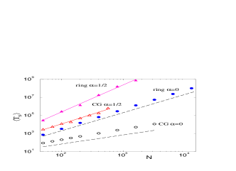
in agreement with simulation results (Fig. 1). Notice that the convergence time for the stubbornest voters, , is of the same order as the consensus time; evidently, this subtlety does not affect our simulation results. Finally, if the lower limit of the distribution of flip rates is strictly greater than zero, then the mean consensus time is linear in .
In one dimension, the HVM organizes into alternating domains of like-minded voters at long times, and consensus is reached when all the intervening (and mobile) domain walls annihilate. This complete annihilation occurs when a single domain wall explores on the order of nodes. Thus consider the motion of a single domain wall between nodes and — all voters to the left of are in state and all other voters are in state . In a time interval , the probabilities that this domain wall hops one step to the right and to the left are, respectively,
| (6) |
The crucial point is that hopping probabilities at adjacent nodes are anti-correlated — if the bias at node is to the right (corresponding to ), then it is more likely that and the bias at node will be to the left. More precisely, for three consecutive rates with the constraint , their relative sizes may equiprobably be SML, SLM, or MLS, where S, M, L denotes the smallest, middle, and largest of these three rates. The latter two cases correspond to a leftward bias between nodes and , which thus occurs with probability 2/3.
With the hopping probabilities and , the mean first-passage time for a particle to travel from to in the finite interval is known NG88 ; L89 ; MK89 :
| (7) |
In the Sinai problem S82 , where the and are independent, identically-distributed random variables, grows as NG88 . For the HVM, the anti-correlated hopping probabilities (6) lead to substantial cancellations in the above product and yields
| (8) |
Using our previous result for , we thus obtain , which agrees well with our numerical simulations shown in Fig. 1(b).
Partisan Voter Model (PVM): Without being pejorative, define state as “democrat” and state as “republican”. In the PVM, each voter has a fixed and innate preference for democrat or republican. Equivalently, each voter experiences its own random field. A voter can therefore exist in one of four states: a “concordant democrat” is a democratic voter in its preferred state, while “discordant democrat” is a democratic voter that happens to be in the state. Complementary definitions apply for “concordant republican” and “discordant republican”.
Denote the densities of these four types of voters as , , , and , respectively. The density of voters that happen to be in the state (current democrats) is . In a single update event, a voter in a social network is randomly selected and it selects a random neighbor. If these two voters are in the same state, nothing happens. If the pair is in different opinion states, the initial voter changes its state as follows:
-
•
if the voter becomes aligned with its preference, the change occurs at rate ;
-
•
if the voter becomes anti-aligned with its preference, the change occurs at rate .
Thus quantifies the strength of the intrinsic preference, or partisanship. If , each voter becomes a zealot that never changes opinion after aligning with its innate preference, while recovers the classic voter model. A similar dichotomous rate arises for catalysis on a disordered surface FKR95 , where surface heterogeneity controls the adsorption rate of different reactants on the surface.
By analyzing the outcomes from all possible pairs of opposite-opinion voters, the rate equations for the densities and in the mean-field limit are:
| (9) | ||||
The equations for and are obtained from (LABEL:ME) by interchanging . Note that , which expresses the conservation of voters of any type.

Let and denote the density of intrinsic democrats and republicans, respectively. For simplicity, we specialize to the symmetric case of , so that the density of democrats of any kind, concordant and discordant, is given by ; similarly, . Using these relations, . In terms of the sum and the difference in the densities of concordant voters, Eqs. (LABEL:ME) simplify to
| (10) | ||||
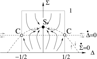
For (classic voter model), , and the average density of voters in either opinion state is conserved. Because , the density of concordant voters is driven to in the final consensus state. For general , there are two fixed points (Fig. 2):
-
•
Self-centered (S): and . Each voter tends to internal concordance at the expense of consensus.
-
•
Consensus (C): and . One half of all the voters are intrinsically concordant.
To infer the global flow in the - plane, we determine the nullclines and (given by and , respectively), and study the linearized rate equations about each fixed point. Both eigenvalues are negative at the self-centered fixed point S, while the eigenvalues have different signs at the consensus fixed points C. Thus if voters have innate preferences, small deviations from the consensus fixed points will grow and the population will be driven to the S fixed point, where each agent tends to align with its innate preference. As the partisanship strength increases, each individual is more likely to be aligned with its innate preference, but with a concomitant lack of consensus.


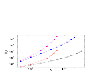
For a finite system, however, the only true fixed points of the stochastic dynamics of the PVM are those that correspond to consensus. Since the flow in the - phase plane is driven away from these fixed points, the time to reach consensus should scale exponentially in the population size. We can understand this behavior easily in one dimension because now the dynamics of single domain walls map exactly to the motion of a particle in a random potential (the Sinai model S82 ). As illustrated in Fig. 3, strings of consecutive democrats or republicans give rise to potential barriers that domain walls have to surmount to annihilate each other and allow the system to reach consensus. In a system of length , the mean time for a domain wall to move a distance therefore scales as S82 ; NG88 ; L89 ; MK89 . Numerical simulations of the PVM on the complete graph and on the one-dimensional periodic lattice (Fig. 4) are consistent with this prediction. We also checked that qualitatively similar behavior arises when the PVM is generalized to allow for heterogeneity in the flip rate of each voter.
To summarize, we extended the voter model to incorporate the realistic features of heterogeneity and partisanship. Both generalizations are characterized by a much slower approach to consensus than in the classic voter model. When voters are partisan, their individual preferences dominate over collectivism, and it is only by exponentially rare events that consensus can ultimately be achieved. These models offer a step toward the quantitative modeling of social phenomena, such as threshold models of collectivism G78 and social experiments on incentive-driven consensus formation KJTW . Particularly interesting behavior seems to arise when the two opinion states are inequivalent; in this situation, partisanship for the unfavorable state may prevent consensus to the favorable state.
Acknowledgements.
We thank James Fowler for a helpful discussion and literature advice, as well as Serge Galam and Gleb Oshanin for relevant references. NM acknowledges financial support by the Grants-in-Aid for Scientific Research (Nos. 20760258 and 20540382) from MEXT, Japan. NG was supported by travel funds from the Direction générale de l’armement. SR acknowledges support from the US National Science Foundation grant DMR0906504.References
- (1) T. M. Liggett, Interacting Particle Systems, (Springer-Verlag, New York, 1985).
- (2) P. L. Krapivsky, Phys. Rev. A 45, 1067 (1992).
- (3) J. D. Gunton, M. San Miguel, and P. S. Sahni, in: Phase Transitions and Critical Phenomena, Vol. 8, eds. C. Domb and J. L. Lebowitz (Academic, NY 1983); A. J. Bray, Adv. Phys. 43, 357 (1994).
- (4) See e.g., C. Castellano, S. Fortunato, and V. Loreto, Rev. Mod. Phys. 81, 591 (2009).
- (5) E. Ben-Naim, L. Frachebourg, and P. L. Krapivsky, Phys. Rev. E 53, 3078 (1996)
- (6) I. Dornic, H. Chaté, J. Chave, and H. Hinrichsen, Phys. Rev. Lett. 87, 045701 (2001).
- (7) V. Sood, S. Redner, Phys. Rev. Lett. 94, 178701 (2005)
- (8) V. Sood, T. Antal, and S. Redner, Phys. Rev. E 77, 041121 (2008).
- (9) J. H. Fowler, C. T. Dawes, and N. A. Christakis, Proc. Natl. Acad. Sci. (USA) 106, 1720 (2009); J. E. Settle, C. T. Dawes, and J. H. Fowler, Polit. Res. Quarterly 62, 601 (2009).
- (10) M. Granovetter, Am. J. Sociol. 83, 1420 (1978).
- (11) M. Mobilia, Phys. Rev. Lett. 91, 028701 (2003); M. Mobilia, A. Petersen, and S. Redner, J. Stat. Mech. P08029, (2007).
- (12) S. Galam and F. Jacobs, Physica A 381, 366 (2007).
- (13) S. Galam, Physica A 238, 66 (1997).
- (14) M. Kearns, S. Judd, J. Tan, and J. Wortman, Proc. Natl. Acad. Sci. (USA) 106, 1347 (2009).
- (15) J. Galambos, The Asymptotic Theory of Extreme Order Statistics (Krieger Publishing Co., Malabar, FL, 1987).
- (16) S. H. Noskowicz and I. Goldhirsch, Phys. Rev. Lett. 61, 500 (1988).
- (17) P. Le Doussal, Phys. Rev. Lett. 62, 3097 (1989).
- (18) K. P. N. Murthy and K. W. Kehr, Phys. Rev. A 40, 2082 (1989).
- (19) Ya. G. Sinai, Theor. Probab. Appl. 27 256 (1982).
- (20) L. Frachebourg, P. L. Krapivsky, and S. Redner, Phys. Rev. Lett. 75, 2891 (1995).