Grafting Rays Fellow Travel Teichmüller Geodesics

Abstract.

Given a measured geodesic lamination on a hyperbolic surface, grafting the surface along multiples of the lamination defines a path in Teichmüller space, called the grafting ray. We show that every grafting ray, after reparameterization, is a Teichmüller quasi-geodesic and stays in a bounded neighborhood of some Teichmüller geodesic.

As part of our approach, we show that grafting rays have controlled dependence on the starting point. That is, for any measured geodesic lamination $\lambda$, the map of Teichmüller space which is defined by grafting along $\lambda$ is ${\tt L}$–Lipschitz with respect to the Teichmüller metric, where ${\tt L}$ is a universal constant. This Lipschitz property follows from an extension of grafting to an open neighborhood of Teichmüller space in the space of quasi-Fuchsian groups.

1. Introduction

Let $S$ be a closed surface with finite genus, possibly with finitely many punctures. Let $X$ be a point in Teichmüller space ${{\mathcal{T}}(S)}$, and let $\lambda$ be a measured geodesic lamination on $X$ of compact support. The pair $X$ and the projective class $[\lambda]$ determines a Teichmüller geodesic ray which starts at $X$ and where the associated vertical foliation is a multiple of $\lambda$ [HM], [Ker1]. Let ${\mathcal{G}}(t,\lambda,X)$, $t\geq 0$, denote the point on this ray whose Teichmüller distance from $X$ is $t$. The pair $X$ and $\lambda$ determines another ray in ${{\mathcal{T}}(S)}$ defined by grafting $X$ along $s\lambda$, for $s\in{\mathbb{R}}_{+}$. We denote the resulting Riemann surface by $\operatorname{gr}(s\lambda,X)$. (See [KT], [Tan], [McM] for background on grafting.)

In this paper we show that each grafting ray stays in a bounded neighborhood of a Teichmüller geodesic:

Theorem A.

Let $X\in{\mathcal{T}}(S)$ be $\epsilon$–thick and let $\lambda$ be a measured geodesic lamination on $X$ with unit hyperbolic length. Then for all $t\geq 0$ we have

$$d_{\mathcal{T}}\Big{(}\operatorname{gr}\big{(}e^{2t}\lambda,X\big{)},{\mathcal{G}}\big{(}t,\lambda,X\big{)}\Big{)}\leq{\tt K}$$

where the constant ${\tt K}$ depends only on $\epsilon$ and the topology of $S$ (it is independent of $\lambda$ and $X$).

Here $d_{\mathcal{T}}$ is the Teichmüller distance and we say that $X\in{\mathcal{T}}(S)$ is $\epsilon$–thick if the injectivity radius of the hyperbolic metric on $X$ is at least $\epsilon$ at every point.

The proof of Theorem A actually produces a bound on the distance that depends continuously on the point in moduli space determined by $X$; the existence of a constant depending only on the injectivity radius is then a consequence of the compactness of the $\epsilon$–thick part of moduli space. However, the dependence on the injectivity radius of $X$ is unavoidable:

Theorem B.

There exists a sequence of points $X_{n}$ in ${{\mathcal{T}}(S)}$ and measured laminations $\lambda_{n}$ with unit hyperbolic length on $X_{n}$ such that for any sequence $Y_{n}$ in ${{\mathcal{T}}(S)}$,

$$\sup_{n,{t\geq 0}}d_{\mathcal{T}}\left(\operatorname{gr}(e^{2t}\lambda_{n},X_{n}),{\mathcal{G}}(t,\lambda_{n},Y_{n})\right)=\infty.$$

We now outline the proof of Theorem A. The main construction (carried out in §§2–4, culminating in Proposition 4.5) produces an explicit family of quasiconformal maps between the Riemann surfaces along a grafting ray and those of a Teichmüller geodesic ray starting from another point $Y\in{\mathcal{T}}(S)$. This is done in the case that $S$ has no punctures. Unfortunately, the quasiconformal constant for these maps and the distance $d_{\mathcal{T}}(X,Y)$ depend on the pair $(X,\lambda)$, whereas for the main theorem we seek a uniform upper bound.

Such a bound is derived from the construction in several steps. First, we show that there exist points $X_{\operatorname{std}}\in{\mathcal{T}}(S)$ for which the quasiconformal constants are uniform over an open set in $\mathcal{ML}(S)$ (§4). Then, using the action of the mapping class group and the co-compactness of the $\epsilon$–thick part of ${\mathcal{T}}(S)$, we show that for any $\epsilon$–thick surface $X$ and any $\lambda\in\mathcal{ML}(S)$ there exists $X_{\operatorname{std}}$ near $X$ for which the uniform estimates apply to $(X_{\operatorname{std}},\lambda)$.

At this point we have proved the main theorem up to moving the base points of both the grafting ray and the Teichmüller geodesic ray by a bounded distance from the given $X\in{\mathcal{T}}(S)$. The proof is concluded by showing that both the grafting and Teichmüller rays starting from these perturbed basepoints fellow travel those starting from the original point $X$.

For the Teichmüller ray case, we use a recent theorem of Rafi [Raf3] (generalizing earlier results of [Mas] and [Iva]) which states that Teichmüller geodesics with the same vertical foliation fellow travel, with a bound on the distance depending only on the thickness $\epsilon$ and the distance between the starting points.

It remains to show that grafting rays in a given direction $\lambda$ fellow travel. In §6 we show that $\lambda$–grafting defines a self-map of Teichmüller space that is uniformly Lipschitz with respect to the Teichmüller metric, and since the Lipschitz constant is independent of $\lambda$, the fellow traveling property of grafting rays follows. The key to this Lipschitz bound is a certain extension of grafting to quasi-Fuchsian groups.

In order describe this extension, we regard grafting as a map

$$\operatorname{gr}:\mathcal{ML}(S)\times{\mathcal{F}}(S)\to{\mathcal{T}}(S),$$

where $\mathcal{ML}(S)$ is the space of measured laminations on $S$ and ${\mathcal{F}}(S)\simeq{\mathcal{T}}(S)$ is the realization of Teichmüller space as the set of marked Fuchsian groups, which is a real-analytic manifold parameterizing hyperbolic structures on $S$. By a construction of Thurston, this map lifts to a projective grafting map $\operatorname{Gr}{\colon\,}\mathcal{ML}(S)\times{\mathcal{F}}(S)\to\mathcal{P}(S)$, where $\mathcal{P}(S)$ is the space of marked complex projective structures.

Interpreting Teichmüller space as the “diagonal” in quasi-Fuchsian space ${\mathcal{QF}}(S)\simeq{\mathcal{T}}(S)\times\overline{{\mathcal{T}}(S)}$, we show that projective grafting extends to a holomorphic map defined on a uniform metric neighborhood of ${\mathcal{F}}(S)$ in ${\mathcal{QF}}(S)$. Here we give ${\mathcal{QF}}(S)$ the Kobayashi metric, which is the sup-product of the Teichmüller metrics on ${\mathcal{T}}(S)$ and $\overline{{\mathcal{T}}(S)}$, and we show:

Theorem C.

There exists ${\tt\delta}>0$ such that projective grafting extends to a map $\operatorname{Gr}{\colon\,}\mathcal{ML}(S)\times{\mathcal{QF}}_{\tt\delta}(S)\to\mathcal{P}(S)$ that is holomorphic with respect to the second parameter, where ${\mathcal{QF}}_{\delta}(S)$ is the open $\delta$–neighborhood of ${\mathcal{F}}(S)$ with respect to the Kobayashi metric on ${\mathcal{QF}}(S)$.

Composing this map $\operatorname{Gr}$ with the forgetful map $\pi{\colon\,}\mathcal{P}(S)\to{\mathcal{T}}(S)$, we also obtain a map $\operatorname{gr}=\pi\circ\operatorname{Gr}{\colon\,}{\mathcal{QF}}_{\tt\delta}(S)\to{\mathcal{T}}(S)$, holomorphic in the first factor, which is the extension that we use in the proof of Theorem A. Note that the original grafting map $\operatorname{gr}{\colon\,}\mathcal{ML}(S)\times{\mathcal{T}}(S)\to{\mathcal{T}}(S)$ is not holomorphic with respect to the usual complex structure on ${\mathcal{T}}(S)$; the holomorphic behavior described in Theorem C can only be seen by considering Teichmüller space as a totally real submanifold of ${\mathcal{QF}}(S)$.

We remark that the existence of a local holomorphic extension of $\operatorname{Gr}(\lambda,{\mathchoice{\mkern 1.0mu\mbox{\raise 2.2pt\hbox{$\centerdot$}}\mkern 1.0mu}{\mkern 1.0mu\mbox{\raise 2.2pt\hbox{$\centerdot$}}\mkern 1.0mu}{\mkern 1.5mu\centerdot\mkern 1.5mu}{\mkern 1.5mu\centerdot\mkern 1.5mu}})$ (or $\operatorname{gr}(\lambda,{\mathchoice{\mkern 1.0mu\mbox{\raise 2.2pt\hbox{$\centerdot$}}\mkern 1.0mu}{\mkern 1.0mu\mbox{\raise 2.2pt\hbox{$\centerdot$}}\mkern 1.0mu}{\mkern 1.5mu\centerdot\mkern 1.5mu}{\mkern 1.5mu\centerdot\mkern 1.5mu}})$) to a neighborhood of a point in ${\mathcal{F}}(S)$ follows easily from results of Kourouniotis or Scannell–Wolf (see §6.1 for details), but that extension to a uniform neighborhood of ${\mathcal{F}}(S)$ (i.e. the existence of ${\tt\delta}$) is essential for application to Theorem A and does not follow immediately from such local considerations.

Using the holomorphic extension of grafting and the contraction of Kobayashi distance by holomorphic maps, we then establish the Lipschitz property for grafting:

Theorem D.

There exists a constant ${\tt L}$ such that for any measured lamination $\lambda\in\mathcal{ML}(S)$, the grafting map $\operatorname{gr}_{\lambda}{\colon\,}{{\mathcal{T}}(S)}\to{{\mathcal{T}}(S)}$ is ${\tt L}$–Lipschitz. That is, given any two points $X$ and $Y$ in ${{\mathcal{T}}(S)}$, we have

$$d_{{\mathcal{T}}}\big{(}\operatorname{gr}(\lambda,X),\operatorname{gr}(\lambda,Y)\big{)}\leq{\tt L}\,d_{{\mathcal{T}}}(X,Y).$$

In §7 we combine the rectangle construction with the fellow traveling properties for grafting and Teichmüller rays to derive the main theorem for compact surfaces. In §8 we show how the preceding argument can be modified to prove Theorem A in the case $S$ has punctures.

Finally, in §9 we construct an example illustrating Theorem B.

Shadows in the curve complex

Given any point $X\in{{\mathcal{T}}(S)}$ and a projective class $[\lambda]$ of a measured geodesic lamination on $X$, there are different ways to geometrically define a ray which starts at $X$ and “heads in the direction of $[\lambda]$”; examples include the Teichmüller ray, the grafting ray, and the line of minima [Ker2]. Given any path in Teichmüller space, by taking the shortest curve on each surface, we get a path in the complex $\mathcal{C}(S)$ of curves of $S$, which is often called the shadow of the original path. Masur and Minsky showed [MM] that the shadow of a Teichmüller geodesic is an unparameterized quasi-geodesic in $\mathcal{C}(S)$. A consequence of Theorem A is that the shadow of a grafting ray remains a bounded distance in $\mathcal{C}(S)$ from the shadow of a Teichmüller geodesic ray. Hence, it follows that the same is true of the grafting ray. In the case of a line of minima, though it may not remain a bounded distance from any Teichmüller geodesic, it was shown [CRS] that its shadow fellow-travels that of its associated Teichmüller geodesic. It is interesting that although these paths are defined in rather different ways, at the level of the curve complex, they are essentially the same.

Related results and references

Using a combinatorial model for the Teichmüller metric, Díaz and Kim showed that the conclusion of Theorem A holds for grafting rays of laminations supported on simple closed geodesics [DK]. However, the resulting bound on distance depends on the geometry of the geodesics in an essential way, obstructing the extension of their method to more general laminations by a limiting argument.

Grafting rays were also studied by Wolf and the second author in [DW], where it was shown that for any $X\in{\mathcal{T}}(S)$, the map $\lambda\mapsto\operatorname{gr}(\lambda,X)$ gives a homeomorphism between $\mathcal{ML}(S)$ and ${\mathcal{T}}(S)$. In particular, Teichmüller space is the union of the grafting rays based at $X$, which are pairwise disjoint. In light of Theorem A, we find that this “polar coordinate system” defined using grafting is a bounded distance from the Teichmüller exponential map at $X$.

Acknowledgments

Some of this work was completed at the Mathematical Sciences Research Institute during the Fall 2007 program “Teichmüller Theory and Kleinian Groups”. The authors thank the institute and the organizers of the program for their hospitality. They also thank the referees for helpful comments which improved the paper.

2. The Orthogonal Foliation to a Lamination

Throughout §§2–7 we assume that $S$ has no punctures. In this section we construct, for every $X\in{\mathcal{T}}(S)$ and every measured lamination $\lambda$, a measured foliation ${\mathcal{H}}(\lambda,X)$ orthogonal to $\lambda$ in $X$. This is a kind of approximation for the horizontal foliation of ${\mathcal{G}}(t,\lambda,X)$, which we do not explicitly know. In the case where $\lambda$ is maximal (that is, the complement of $\lambda$ is a union of ideal triangles) the measured foliation is equivalent to the horocyclic foliation constructed by Thurston in [Thu].

A measured foliation orthogonal to $\lambda$

Let $g$ be a geodesic in ${\mathbb{H}}^{2}$. Consider the closest point projection map onto $g$, which takes each point in ${\mathbb{H}}^{2}$ to the point on $g$ to which it is closest. The fibers of the projection foliate ${\mathbb{H}}^{2}$ by geodesics perpendicular to $g$. Analogously, if $\{g_{i}\}$ is a collection of disjoint geodesics, then the closest point projection to $\cup g_{i}$ is well-defined, except at the points that are equidistant to two or more geodesics in $\{g_{i}\}$. These points form a (possibly disconnected) graph where the edges are geodesic segments, rays, or lines. The fibers of the projection foliate ${\mathbb{H}}^{2}$ by piecewise geodesics.

The lamination $\lambda$ lifts to a set $\widetilde{\lambda}$ of disjoint infinite geodesics which is invariant under deck transformations. Let $\widetilde{\theta}$ be the graph of points where the closest point projection to $\widetilde{\lambda}$ is not well-defined and let $\theta$ be the projection of $\widetilde{\theta}$ to $X$. We call the set $\theta=\theta(\lambda,X)$ the singular locus of the closest point projection map. As above, the fibers defined by the projection provides a foliation of ${\mathbb{H}}^{2}$ which projects down to a foliation of $X$. Thus we obtain a singular foliation ${\mathcal{H}}={\mathcal{H}}(\lambda,X)$ on $X$ orthogonal to $\lambda$. The foliation has singularities at the vertices of $\theta$, where the number of prongs at a singularity coincides with the valence of the vertex. The leaves of ${\mathcal{H}}$ are piecewise geodesics whose non-smooth points lie on $\theta$. For later purposes, we prefer to maintain the non-smooth structure of ${\mathcal{H}}$ along $\theta$. A leaf of ${\mathcal{H}}$ that joins two vertices is called a saddle connection.

Proposition 2.1.

The hyperbolic arc-length along $\lambda$ induces a transverse measure on ${\mathcal{H}}(\lambda,X)$.

Proof.

Let $\eta$ be a smooth embedded arc in $X$. First suppose that the interior of $\eta$ is contained in a component of $X\setminus\theta$ (the endpoints of $\eta$ may be contained in $\theta$) and that at every interior point, $\eta$ is transverse to ${\mathcal{H}}$. Let $\widetilde{\eta}$ be a lift of $\eta$. Then the closest point projection onto $\widetilde{\lambda}$ projects $\widetilde{\eta}$ to an arc on a leaf of $\widetilde{\lambda}$. (In the case that an endpoint of $\widetilde{\eta}$ is in $\widetilde{\theta}$, project the endpoint to the same leaf of $\widetilde{\lambda}$ as the interior points.) Define the measure on $\eta$ to be the length of this arc. In the case that $\eta$ is contained in $\theta$, observe that although the closest point projection of $\widetilde{\eta}$ to $\widetilde{\lambda}$ is not well-defined, any choice of projection has the same length because $\widetilde{\theta}$ is equidistant to the corresponding leaves of $\widetilde{\lambda}$. Define the measure on $\eta$ to be the length of this arc. If the interior of $\eta$ intersects $\theta$ at a point $p$, we say $\eta$ is transverse to ${\mathcal{H}}$ at $p$ if, on a small circle $C$ centered at $p$, the points of $\eta\cap C$ separate the points of $\ell\cap C$, where $\ell$ is the leaf of ${\mathcal{H}}$ through $p$. In general, if $\eta$ is transverse to ${\mathcal{H}}$ at every point, we define the ${\mathcal{H}}$-measure of $\eta$ to be the sum of the ${\mathcal{H}}$–measures of the subarcs $\cup[\eta\cap(X\setminus\theta)]$ and any subarcs in $\eta\cap\theta$. In this way, we equip ${\mathcal{H}}$ with a transverse measure that coincides with arc-length along $\lambda$. ∎

Note that neither ${\mathcal{H}}$ nor its transverse measure depends in any way on the measure on $\lambda$.

3. Rectangle decomposition

We now describe a decomposition of $X$ into rectangles using the orthogonal foliation ${\mathcal{H}}={\mathcal{H}}(\lambda,X)$.

Choose an arc $\omega$ contained in $\theta$ that contains no singularities of $\theta$. For every point $p$ on $\omega$ and a choice of normal direction to $\omega$, consider the arc of ${\mathcal{H}}$ starting from $p$ in that direction. By Poincaré recurrence (see for example [FLP, §5.1]), this arc either ends at a singular point of $\theta$ or intersects $\omega$ again. We call such an arc exceptional if it intersects a singular point of $\theta$ or an endpoint of $\omega$ before intersecting the interior of $\omega$. In particular we consider any arc starting from an endpoint of $\omega$ to be exceptional. Let $P\subset\omega$ denote the set of endpoints of exceptional arcs. Label the normal directions of $\omega$ as $n_{1},n_{2}$. Then $P=P_{1}\cup P_{2}$, where $P_{i}$ corresponds to endpoints of exceptional arcs in the normal direction $n_{i}$.

The first return map of ${\mathcal{H}}$ is defined on the set of pairs $(p,n_{i})$ where $p\in\omega$, $i\in\{1,2\}$, and $p\notin P_{i}$. That is, the first return map is naturally a self-map of

$$\big{(}\omega\setminus P_{1}\big{)}\times\{n_{1}\}\cup\big{(}\omega\setminus P_{2}\big{)}\times\{n_{2}\}.$$

An open interval of $\omega\setminus P_{i}$ flows along ${\mathcal{H}}$ in the direction $n_{i}$ until it returns to another (possibly overlapping) interval of $\omega$ sweeping out a rectangle that has two edges attached to $\omega$ (see Figure 1). We refer to it as a rectangle, despite the fact that the edges along ${\mathcal{H}}$ are jagged, because the endpoints of the edges which are attached to $\omega$ give four distinguished points on the boundary. We call these points the vertices of the rectangle.

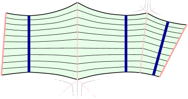
Figure 1. A rectangle $R$ foliated by leaves of ${\mathcal{H}}$ in the case where $\lambda$ is a weighted multicurve (of which three segments are shown in bold). The leaves of ${\mathcal{H}}$ are piecewise geodesics, smooth away from $\theta$ and orthogonal to $\lambda$ at each intersection. The left and right edges of $R$ are contained in $\omega$.

If ${\mathcal{H}}(\lambda,X)$ has no saddle connections, this decomposes $X$ into a union of rectangles. If ${\mathcal{H}}(\lambda,X)$ has saddle connections, then the union of the rectangles may only be a subsurface of $X$, whose boundary is made of saddle connections. We will however, assume below in (H1) that ${\mathcal{H}}(\lambda,X)$ has no saddle connections.

The interiors of the rectangles are disjoint and contain no singularities. For every rectangle $R$, we call the pair of opposite edges that are sub-arcs of $\omega$ the vertical edges of $R$. The refer to the other pair of opposite edges, that are sub-arcs of leaves of ${\mathcal{H}}$, as the horizontal edges of $R$. The rectangle decomposition obtained from a transversal $\omega$ in this way will be denoted by $\mathcal{R}(\omega,\lambda,X)$.

3.1. Topological stability of the decomposition

Suppose $\mu$ is a maximal measured lamination, that is, the complement of $\mu$ is a union of ideal triangles. The foliation $\mathcal{H}(\mu,X)$ has a three-prong singularity at the center of each ideal triangle. If $\lambda$ is close to $\mu$ in the usual weak topology of $\mathcal{ML}(S)$ then, because $\mu$ is maximal, the lamination $\lambda$ is also close to $\mu$ in the Hausdorff topology (see [Thu, pp. 24–25] [Wei]). Since $\mathcal{H}(\lambda,X)$ varies continuously with the support of $\lambda$, the singularities of $\mathcal{H}(\lambda,X)$ remain isolated from one another and are the same in number and type. Similarly, the part of the singular graph $\theta(\mu,X)$ that lies outside a small neighborhood of the support of $\mu$ will be close (in the $C^{1}$ topology of embedded graphs) to the corresponding part of $\theta(\lambda,X)$.

We emphasize that the constructions above are not continuous in any neighborhood of $\mu$ in the measure topology of $\mathcal{ML}(S)$; rather, maximality of $\mu$ implies continuity at $\mu$, since for maximal laminations, convergence in measure and in the Hausdorff sense are the same.

Let us further assume that ${\mathcal{H}}(\mu,X)$ and $\omega$ satisfy:

1. The foliation ${\mathcal{H}}(\mu,X)$ has no saddle connections (and in particular, it is minimal).

2. The horizontal sides of rectangles in ${\mathcal{R}}(\omega,\mu,X)$ containing the endpoints of $\omega$ do not meet the singularities of ${\mathcal{H}}(\mu,X)$.

Then we can conclude that for $\lambda$ sufficiently close to $\mu$ and an arc $\omega_{\lambda}\subset\theta(\lambda,X)$ sufficiently close to $\omega$, the rectangle decomposition ${\mathcal{R}}(\omega_{\lambda},\lambda,X)$ is well-defined and is topologically equivalent (i.e. isotopic) to ${\mathcal{R}}(\omega,\mu,X)$. First, note that $\omega_{\lambda}$ is still disjoint from $\lambda$ and transverse to ${\mathcal{H}}(\lambda,X)$. Moreover, the condition (H1) ensures that every point in $P_{1}$ and $P_{2}$ corresponds to a unique point in $\omega_{\lambda}$. (Note that if ${\mathcal{H}}(\mu,X)$ had a saddle connection, both saddle points would project to the same point in $\omega$. But the corresponding points in ${\mathcal{H}}(\lambda,X)$ may project to different points in $\omega_{\lambda}$.) Thus the rectangle decompositions ${\mathcal{R}}(\omega,\mu,X)$ and ${\mathcal{R}}(\omega_{\lambda},\lambda,X)$ are topologically equivalent.

In order to analyze rectangle decompositions for laminations near a given one, it will be convenient to work with an open neighborhood $U\subset\mathcal{ML}(S)$ of $\mu$ and to extend the transversal $\omega$ to a family of transversals $\{\omega_{\lambda}:\lambda\in U\}$. We require that this family satisfy the conditions:

1. For each $\lambda\in U$, the arc $\omega_{\lambda}$ lies in the singular locus $\theta(\lambda,X)$, and its endpoints are disjoint from the vertices of $\theta(\lambda,X)$.

2. The family of transversals is continuous at $\mu$, meaning that for any $\lambda_{n}\in U$ such that $\lambda_{n}\to\mu$ in the measure topology, the transversals $\omega_{\lambda_{n}}$ converge to $\omega=\omega_{\mu}$ in the $C^{1}$ topology.

Note that for any maximal lamination $\mu\in\mathcal{ML}(S)$, we can start with a transversal $\omega$ in an edge of its associated singular locus and construct a family satisfying the conditions above on some neighborhood of $\lambda$ in $\mathcal{ML}(S)$. For example, we can take $\omega_{\lambda}$ to be the arc in $\theta(\lambda,X)$ whose endpoints are closest to those of $\omega$. The $C^{1}$ convergence of these arcs as $\lambda\to\mu$ follows from the convergence of the singular graphs, once we choose the neighborhood of $\lambda$ in $\mathcal{ML}(S)$ so that the original arc $\omega_{\mu}$ has a definite distance from the support of any lamination in the neighborhood.

3.2. Geometric stability of the decomposition

To quantify the geometry of a rectangle decomposition, rather than its topology, we introduce parameters describing aspects of the shape of a rectangle $R\in{\mathcal{R}}(\omega,\mu,X)$. Let ${\mathcal{H}}={\mathcal{H}}(\mu,X)$ and define

$$0pt_{R}(\mu)=\text{${\mathcal{H}}$--measure of a vertical edge of $R$}.$$

By construction, the vertical edges of $R$ have the same ${\mathcal{H}}$-measure, so this is well-defined, and is equal to the length of any arc in $R\cap\mu$.

Since we are assuming ${\mathcal{H}}(\mu,X)$ has no saddle connections, each horizontal edge of $R$ either contains exactly one singularity of ${\mathcal{H}}$ or does not contain any singularities, but ends at an endpoint of $\omega$. In the former case, the singularity divides the edge into two horizontal half-edges. Although in the latter case, the edge is not divided, we nonetheless refer to it as a horizontal “half-edge” and include it in the set ${\mathcal{I}}_{R}$ of horizontal half-edges of $R$. Define

$${\tt l}_{R}(\mu)=\max_{I\in\mathcal{I}_{R}}\ell(I),$$

where $\ell(I)$ denotes the hyperbolic length of $I$.

Also define

$${\tt m}_{R}(\mu)=\min_{I\in\mathcal{I}_{R}}\operatorname{i}(I,\mu),$$

where $\operatorname{i}({\mathchoice{\mkern 1.0mu\mbox{\raise 2.2pt\hbox{$\centerdot$}}\mkern 1.0mu}{\mkern 1.0mu\mbox{\raise 2.2pt\hbox{$\centerdot$}}\mkern 1.0mu}{\mkern 1.5mu\centerdot\mkern 1.5mu}{\mkern 1.5mu\centerdot\mkern 1.5mu}},{\mathchoice{\mkern 1.0mu\mbox{\raise 2.2pt\hbox{$\centerdot$}}\mkern 1.0mu}{\mkern 1.0mu\mbox{\raise 2.2pt\hbox{$\centerdot$}}\mkern 1.0mu}{\mkern 1.5mu\centerdot\mkern 1.5mu}{\mkern 1.5mu\centerdot\mkern 1.5mu}})$ is the intersection number with the transverse measure of $\mu$.

We consider the variation of the rectangle parameters over $U$, continuing under the assumption that (H1),(H2),(T1),(T2) hold. By construction, the parameters $0pt_{R}(\mu)$ and ${\tt l}_{R}(\mu)$ depend continuously on the foliation ${\mathcal{H}}(\mu,X)$ and on a compact part of the the singular locus $\theta(\mu,X)$, both of which vary continuously with the support of $\mu$ in the Hausdorff topology. Thus both of these parameters are continuous at a maximal lamination. And, ${\tt m}_{R}(\mu)$ varies continuously with $\mu$.

For future reference, we summarize this discussion in the following lemma:

Lemma 3.1.

Suppose $\mu$ is maximal and $\omega$ is a transversal such that the pair satisfy (H1) and (H2) above. Then there is a neighborhood $U$ of $\mu$ in $\mathcal{ML}(S)$ and a family of transversals satisfying (T1) and (T2) such that the associated rectangle decompositions are all topologically equivalent, and such that for any $\lambda\in U$, we have:

(1) $$\begin{split}{\tt l}_{R}(\lambda)&<2\,{\tt l}_{R}(\mu);\\ {\tt m}_{R}(\lambda)&>\frac{{\tt m}_{R}(\mu)}{2};\\ 0pt_{R}(\lambda)&>\frac{0pt_{R}(\mu)}{2}.\end{split}$$

4. Construction of a Quasiconformal Map

Our plan is to use the rectangle decomposition to define a quasiconformal map from the grafting ray to a Teichmüller ray. In order to bound the quasiconformal constant, however, we need control over the shapes of the rectangles. Thus we first consider a standard surface $X_{\operatorname{std}}$ for which the rectangle decomposition is well-behaved.

We will need the following lemma.

Lemma 4.1.

For every maximal lamination $\mu$, the set $V_{\mu}$ of Riemann surfaces $Y\in{\mathcal{T}}(S)$ where ${\mathcal{H}}(\mu,Y)$ has no saddle connections is the intersection of a countable number of open dense subsets of ${\mathcal{T}}(S)$. For each $Y\in V_{\mu}$, there is an arc $\omega$ in $\theta(\mu,Y)$ satisfying (H2) above.

Proof.

Since every point in ${{\mathcal{T}}(S)}$ comes with a marking, we can consider $\mu$ and ${\mathcal{H}}(\mu,X)$ as a measured lamination and a measured foliation on $S$, respectively. Since $\mu$ is maximal, there is one singularity of ${\mathcal{H}}(\mu,X)$ contained in each complementary ideal triangle. Let ${\mathcal{A}}={\mathcal{A}}(\mu)$ be the set of homotopy classes of arcs connecting the singular points of ${\mathcal{H}}(\mu,X)$. For any $Y\in{{\mathcal{T}}(S)}$, the set of homotopy classes of arcs connecting the singular points of ${\mathcal{H}}(\mu,Y)$ is identified with ${\mathcal{A}}$ via the marking map $S\to Y$.

Let $\alpha$ be an arc in ${\mathcal{A}}$, and consider the set $V_{\alpha}$ of points $Y\in{{\mathcal{T}}(S)}$ such that $\alpha$ is not a saddle connection of ${\mathcal{H}}(\mu,Y)$. Suppose that $Z$ is in the complement of this set $V^{c}_{\alpha}$. Let $Z_{t}$ be the image of $Z$ after applying a left earthquake along the measured lamination $t\mu$ and let ${\mathcal{H}}_{t}={\mathcal{H}}(\mu,Z_{t})$. An arc in ${\mathcal{A}}$ appears as a saddle connection of ${\mathcal{H}}_{t}$ if its ${\mathcal{H}}_{t}$–measure is zero. But the ${\mathcal{H}}_{t}$–measure of each arc is a linear function of $t$; by the definition of the earthquake flow, the ${\mathcal{H}}_{t}$–measure of such an arc is equal to its ${\mathcal{H}}_{0}$ measure plus its $\mu$–measure times $t$. Since $\mu$ is maximal, every arc in ${\mathcal{A}}$ has to intersect $\mu$ and hence the ${\mathcal{H}}_{t}$–measure cannot remain constant. Therefore, $Z_{t}$ is in $V_{\alpha}$ for every $t>0$. Since we can apply the same argument for right earthquakes, it follows that $V^{c}_{\alpha}$ is a closed subset of ${{\mathcal{T}}(S)}$ of co-dimension at least one. Thus, $V_{\alpha}$ is an open dense subset of ${{\mathcal{T}}(S)}$. Since ${\mathcal{A}}$ consists of a countable number of elements, the intersection

$$V_{\mu}=\cap_{\alpha\in{\mathcal{A}}}V_{\alpha}$$

is an intersection of a countable number of open dense subset of ${{\mathcal{T}}(S)}$.

For $Y\in V_{\mu}$, choose an arc $\omega_{0}\in\theta(\mu,Y)$. There are finitely many leaves of ${\mathcal{H}}(\mu,Y)$ that contain singularities, and these intersect $\omega_{0}$ in a countable set of points. Any sub-interval $\omega\subset\omega_{0}$ whose endpoints are in the complement of this set will satisfy (H2). ∎

4.1. The standard surface

Consider a pair of pseudo-Anosov maps $\varphi$ and ${\overline{\varphi}}$, so that the associated stable lamination $\nu$ and ${\overline{\nu}}$ are distinct and maximal. We perturb $X$ to a Riemann surface $X_{\operatorname{std}}$ so that both orthogonal foliations ${\mathcal{H}}={\mathcal{H}}(\nu,X_{\operatorname{std}})$ and ${\overline{\mathcal{H}}}={\mathcal{H}}({\overline{\nu}},X_{\operatorname{std}})$ satisfy (H1). This is possible because, by Lemma 4.1, the intersection of $V_{\nu}$ and $V_{{\overline{\nu}}}$ is still dense and hence is non-empty.

Let $\theta$ and ${\overline{\theta}}$ be the singular loci of ${\mathcal{H}}$ and ${\overline{\mathcal{H}}}$ respectively. We choose arcs $\omega_{\operatorname{std}}$ and ${\overline{\omega}_{\operatorname{std}}}$ contained in $\theta$ and ${\overline{\theta}}$ respectively, satisfying (H2). Let $U$ and ${\overline{U}}$ be open neighborhoods of $\nu$ and ${\overline{\nu}}$ as in Lemma 3.1. By making $U$ and ${\overline{U}}$ smaller if necessary, we can assume that they are disjoint. Let $U_{\operatorname{std}}=U\cup{\overline{U}}$, and for $\lambda\in U_{\operatorname{std}}$, let $\mathcal{R}(\lambda)$ denote the rectangle decomposition ${\mathcal{R}}(\omega_{\lambda},\lambda,X_{\operatorname{std}})$.

For $R\in{\mathcal{R}}(\nu)$, we know that ${\tt l}_{R}>0$ and $0pt_{R}>0$ (this is true for any non-degenerate rectangle). An arc contained in a leaf of ${\mathcal{H}}$ connecting two points in $\theta$ must intersect $\lambda$. Therefore, such an arc connecting $\omega_{\operatorname{std}}$ to itself or to a singular point of ${\mathcal{H}}$ (which also lies in $\theta$) has to have a positive $\nu$ measure. Hence, ${\tt m}_{R}$ is also positive. Similar statements are true for ${\overline{\nu}}$. Define

$${\tt L} =\max\big{\{}{\tt l}_{R}:R\in{\mathcal{R}}(\lambda),\ \lambda\in U_{\operatorname{std}}\big{\}};$$

(2) $${\tt M} =\min\big{\{}{\tt m}_{R}:R\in{\mathcal{R}}(\lambda),\ \lambda\in U_{\operatorname{std}}\big{\}};$$

$${\tt H} =\min\,\big{\{}0pt_{R}:R\in{\mathcal{R}}(\lambda),\ \lambda\in U_{\operatorname{std}}\big{\}}.$$

Then, by Lemma 3.1, ${\tt H}$, ${\tt M}$ and ${\tt L}$ are finite and positive. These constants give uniform control over the shapes of all rectangles in any rectangle decomposition ${\mathcal{R}}(\lambda)$ for $\lambda\in U_{\operatorname{std}}$.

For the rest of this section we restrict our attention to laminations $\lambda$ in $U_{\operatorname{std}}$ only. We prove that the grafting ray $\operatorname{gr}(s\lambda,X_{\operatorname{std}})$ fellow travels a Teichmüller geodesic with constants depending on $X_{\operatorname{std}}$, $\omega_{\operatorname{std}}$, ${\overline{\omega}_{\operatorname{std}}}$ and $U_{\operatorname{std}}$ but not on $\lambda$ (Proposition 4.5).

4.2. Rectangle decomposition of $\operatorname{gr}(s\lambda,X_{\operatorname{std}})$.

The rectangle decomposition ${\mathcal{R}}(\lambda)$ can be extended to a rectangle decomposition of the grafted surface $\operatorname{gr}(s\lambda,X_{\operatorname{std}})$ that is adapted to its Thurston metric rather than the hyperbolic metric that uniformizes it. The surface $\operatorname{gr}(s\lambda,X_{\operatorname{std}})$ is obtained by cutting $X_{\operatorname{std}}$ along the isolated leaves of $\lambda$ and attaching a cylinder of the appropriate thickness in their place. That is, the complement of the isolated leaves of $\lambda$ in $X_{\operatorname{std}}$ is canonically homeomorphic to the complement of the corresponding cylinders in the grafted surface. However, when $\lambda$ has leaves that are not isolated, the complement of the cylinders changes as a metric space. The length of an arc in the Thurston metric of $\operatorname{gr}(s\lambda,X_{\operatorname{std}})$ disjoint from the cylinders is its hyperbolic length plus its $s\lambda$–measure.

The rectangle decomposition ${\mathcal{R}}(\lambda)$ defines a rectangle decomposition ${\mathcal{R}}_{s}(\lambda)$ of $\operatorname{gr}(s\lambda,X_{\operatorname{std}})$ as follows. A rectangle $R$ in ${\mathcal{R}}(\lambda)$ is extended to a rectangle $R_{s}$ by cutting along each isolated arc in $\lambda\cap R$ and inserting a Euclidean rectangle of width $s$ times the original $\lambda$–measure carried by the arc, as in Figure 2. Then ${\mathcal{R}}_{s}(\lambda)$ is the collection of rectangles $R_{s}$. The foliation ${\mathcal{H}}$ can be extended to a foliation ${\mathcal{H}}_{s}$ of $\operatorname{gr}(s\lambda,X_{\operatorname{std}})$; inside the cylinders corresponding to isolated leaves, ${\mathcal{H}}_{s}$ is the foliation by geodesic arcs (in the Euclidean metric on the cylinder) that are perpendicular to the boundaries of the cylinder.

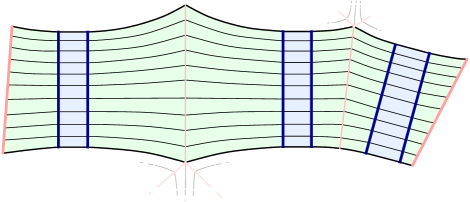
Figure 2. The rectangle decomposition extends naturally to the grafted surface, replacing isolated arcs of $R\cap\lambda$ with Euclidean rectangles contained in the grafted annuli.

4.3. Foliation parallel to $\lambda\cup\theta$

Let $R$ be a rectangle in ${\mathcal{R}}(\lambda)$. We foliate $R$ with geodesic arcs parallel to $\lambda\cup\theta$ as follows. A component of $R\setminus(\lambda\cup\theta)$ is a geodesic quadrilateral that has a pair of opposite sides lying in $\theta$ and $\lambda$ respectively. Consider this quadrilateral in the hyperbolic plane, where these opposite sides are contained in a pair of disjoint infinite geodesics $g_{1}$ and $g_{2}$. If $g_{1}$ and $g_{2}$ do not meet at infinity, the region between them can be foliated by geodesics that are perpendicular to the common perpendicular of $g_{1}$ and $g_{2}$. If $g_{1}$ and $g_{2}$ meet at infinity, the region between them can be foliated by geodesics sharing the same endpoint at infinity. This foliation restricts to a foliation of the quadrilateral by arcs. Applying the same construction for each component in each rectangle, we obtain a foliation ${\mathcal{V}}={\mathcal{V}}(\omega_{\lambda},\lambda,X_{\operatorname{std}})$ of $X_{\operatorname{std}}$ that is transverse to ${\mathcal{H}}$. Note that, unlike ${\mathcal{H}}$, the vertical foliation ${\mathcal{V}}$ does not have a natural transverse measure.

Similar to ${\mathcal{H}}$, the foliation ${\mathcal{V}}$ can be extended to a foliation ${\mathcal{V}}_{s}$ of the grafted surface $\operatorname{gr}(s\lambda,X_{\operatorname{std}})$; inside cylinders corresponding to isolated leaves, ${\mathcal{V}}$ extends as the orthogonal foliation to ${\mathcal{H}}_{s}$.

4.4. Projections along ${\mathcal{V}}_{s}$.

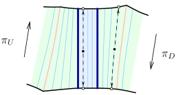
Figure 3. A portion of a rectangle $R_{s}$ foliated by leaves of ${\mathcal{V}}_{s}$ in the case where $\lambda$ is a weighted multi-curve. The central rectangle is part of an annulus that has been grafted along $\lambda$. The top and bottom edges of $R_{s}$ are arcs in the leaves of ${\mathcal{H}}_{s}$.

Let $R$ be a rectangle in ${\mathcal{R}}(\lambda)$. Orient $R$ so that the notions of up, down, left and right are defined; these are still well defined for the grafted rectangle $R_{s}\in{\mathcal{R}}_{s}(\lambda)$. We assume that the top and the bottom edges are horizontal and the left and the right edges are vertical.

Fixing the rectangle $R_{s}$, we define the map $\operatorname{\pi_{D}}$ from $R_{s}$ to the bottom edge of $R_{s}$ to be the projection downward along the leaves of ${\mathcal{V}}_{s}$ and the map $\operatorname{\pi_{U}}$ from $R_{s}$ to the top edge of $R_{s}$ to be the projection upward along the leaves of ${\mathcal{V}}_{s}$ (see Figure 3). Also, define a map $h{\colon\,}R_{s}\to{\mathbb{R}}_{+}$ to be the height. That is, for $p\in R_{s}$, $h(p)$ is the ${\mathcal{H}}_{s}$–measure of any arc (transverse to ${\mathcal{H}}$) connecting $p$ to the bottom edge of $R_{s}$.

Lemma 4.2.

There is a constant ${\tt B}>0$ depending only on $X_{\operatorname{std}}$ such that, for every $\lambda\in U_{\operatorname{std}}$ and $R_{s}\in{\mathcal{R}}_{s}(\lambda)$ equipped with the Thurston metric, the following holds.

1. The maps $\operatorname{\pi_{U}}$ and $\operatorname{\pi_{D}}$ are ${\tt B}$–Lipschitz. Furthermore, the restrictions of these maps to a leaf of ${\mathcal{H}}_{s}$ are ${\tt B}$–bi-Lipschitz.

2. The map $h$ is ${\tt B}$–Lipschitz. Furthermore, the restriction of $h$ to a leaf of ${\mathcal{V}}_{s}$ is ${\tt B}$–bi-Lipschitz.

Proof.

The lemma clearly holds for the interior of added cylinders with ${\tt B}=1$ as $\operatorname{\pi_{U}}$, $\operatorname{\pi_{D}}$ and $h$ are just Euclidean projections. As mentioned before, in the complement of these added cylinders, the Thurston length of an arc in $R_{s}$ is the sum of the hyperbolic length of this arc and its $s\lambda$–transverse measure. As one projects an arc up or down, the $s\lambda$–measure does not change. Therefore, to prove the first part of the lemma, we need only to prove it for the restriction of $\operatorname{\pi_{U}}$ and $\operatorname{\pi_{D}}$ to every component of $R\setminus(\lambda\cup\theta)$. Similarly, proving part two in each component of $R\setminus(\lambda\cup\theta)$ is also sufficient. This is because showing $h$ is Lipschitz with respect to the hyperbolic metric implies that it is Lipschitz with respect to the Thurston metric as well (since the Thurston metric is pointwise larger [Tan, Prop. 2.2]). Also, the leaves of ${\mathcal{V}}$ reside in one component.

Let $Q$ be a component of $R\setminus(\lambda\cup\theta)$. We know that $Q$ is a hyperbolic quadrilateral with one vertical edge $e_{1}$ in $\lambda$ and the other $e_{2}$ in $\theta$. Since ${\mathcal{H}}$ was defined by closest point projection to $\lambda$, the top and bottom edges of $Q$ make an angle of $\pi/2$ with the edge $e_{1}$. The hyperbolic length of $e_{1}$ is bounded by the hyperbolic length of $\omega$ and the maximum distance between $e_{1}$ and $e_{2}$ is bounded above by the diameter of $X_{\operatorname{std}}$. That is, fixing $X_{\operatorname{std}}$ and $\omega$, the space of possible shapes (after including the degenerate cases) is compact in Hausdorff topology. For each possible quadrilateral $Q$, the maps in question are Lipschitz (including the degenerate cases where the length of $e_{1}$ is zero, or, $e_{1}$ and $e_{2}$ coincide) and the Lipschitz constants vary continuously with shape. Hence, the maps $\operatorname{\pi_{U}}$, $\operatorname{\pi_{D}}$ and $h$ are uniformly Lipschitz.

Also, the restriction of $\operatorname{\pi_{U}}$ and $\operatorname{\pi_{D}}$ to leaves of ${\mathcal{H}}$ are always bijections and have positive derivatives and the restriction of $h$ to a leaf of ${\mathcal{V}}$ is a bijection and has a positive derivative. Thus, there is a uniform lower bound for these derivatives and hence they are uniformly bi-Lipschitz maps. ∎

4.5. Mapping to a singular Euclidean surface

For each rectangle $R_{s}$ in ${\mathcal{R}}_{s}(\lambda)$ consider a corresponding Euclidean rectangle $E_{s}$ with width equal to the $s\lambda$–measure of the horizontal edges of $R_{s}$ and height equal to the ${\mathcal{H}}_{s}$–measure of the vertical edge. Recall that a horizontal edge of a rectangle $R_{s}$ is divided into two (or one; see §3.2) horizontal half-edges; the set of horizontal half-edges of $R_{s}$ is denoted by ${\mathcal{I}}_{R_{s}}$. We also mark a special point on each the horizontal edge of $E_{s}$, dividing it into horizontal half-edges, so that the Euclidean length of the interval associated to $I\in{\mathcal{I}}_{R_{s}}$ is equal to $\operatorname{i}(s\lambda,I)$.

We fix a correspondence between horizontal half-edges of $R_{s}$ and $E_{s}$. Glue the rectangles $E_{s}$ along these horizontal half-edges and the vertical edges with Euclidean isometries in the same pattern as the rectangles $R_{s}$ are glued in ${\mathcal{R}}_{s}(\lambda)$. Each horizontal half-edge $I$ appears in two rectangles, but $\operatorname{i}(s\lambda,I)$ is independent of which rectangle we choose. Similarly, the vertical edges appear in two rectangles each, but their ${\mathcal{H}}_{s}$–measures are independent of the choice of the rectangle. Hence the lengths of corresponding intervals in $E_{s}$ match and the gluing is possible; it results in a singular Euclidean surface ${\mathcal{E}}_{s}$. Our goal in this section is to define a quasiconformal map $F$ between $\operatorname{gr}(s\lambda,X_{\operatorname{std}})$ and ${\mathcal{E}}_{s}$.

Consider the rectangles in ${\mathcal{R}}_{s}(\lambda)$ as sitting in $\operatorname{gr}(s\lambda,X_{\operatorname{std}})$ and the corresponding rectangles as sitting in ${\mathcal{E}}_{s}$. The horizontal half-edges and the vertical edges of the rectangles form a graph in $\operatorname{gr}(s\lambda,X_{\operatorname{std}})$. First, we define a map $f_{s}$ from this graph to the associated graph in ${\mathcal{E}}_{s}$. Note that, for the gluing to work, the map should depend on the edge only and not on the choice of rectangle containing it. We map any horizontal half-edge $I\in{\mathcal{I}}_{R_{s}}$ of the rectangle $R_{s}$ linearly onto the associated interval in $E_{s}$, where we take $I$ to be equipped with the induced Thurston metric. We map a vertical edge $J$ to the associated vertical edge in $E_{s}$ so that the ${\mathcal{H}}_{s}$–measure is preserved. Note that $f_{s}$ is distance non-increasing.

Now that the map $f_{s}$ is defined on the $1$–skeleton, we extend it to a map

$$F_{s}{\colon\,}\operatorname{gr}(s\lambda,X_{\operatorname{std}})\to{\mathcal{E}}_{s},$$

as follows: for each rectangle $R_{s}$, we send leaves of ${\mathcal{V}}$ to geodesic segments in $E_{s}$ so that ${\mathcal{H}}_{s}$ is preserved. More precisely, for every point $p\in R_{s}$, consider the points $q=f_{s}(\operatorname{\pi_{U}}(p))$ and $q^{\prime}=f_{s}(\operatorname{\pi_{D}}(p))$. Then, let $F_{s}(p)$ be the point in the segment $[q,q^{\prime}]$ whose distance from the bottom edge of $E_{s}$ is $h(p)$. We observe the following:

Lemma 4.3.

The slope of the segment $[q,q^{\prime}]$ is uniformly bounded below.

Proof.

Consider the rectangle $E_{s}$ in ${\mathbb{R}}^{2}$ with the horizontal and the vertical edges parallel to the $x$–axis and the $y$–axis respectively and the bottom left vertex at the origin. The height of $R_{s}$ is at least ${\tt H}$, so the same is true of $E_{s}$. Hence, we need to show that the $x$–coordinates of $q$ and $q^{\prime}$ differ by at most a bounded amount.

Let $I$ be the interval connecting the top left vertex of $R_{s}$ to $\operatorname{\pi_{U}}(p)$ and let $I^{\prime}$ be the interval connecting the bottom left vertex of $R_{s}$ to $\operatorname{\pi_{D}}(p)$. Note that, $\operatorname{i}(s\lambda,I)=\operatorname{i}(s\lambda,I^{\prime})$. Also, the Thurston length of $I$ is equal to $\operatorname{i}(s\lambda,I)$ plus the hyperbolic length of $I$, which is bounded above by ${\tt L}$ and the same holds for $I^{\prime}$. Therefore, the Thurston lengths of $I$ and $I^{\prime}$ differ by at most $2{\tt L}$. It remains to be shown that the difference between the $x$–coordinate of $q$ and the Thurston length of $I$ and the difference between the $x$–coordinate of $q^{\prime}$ and the Thurston length of $I^{\prime}$ are uniformly bounded.

To see this last assertion note that, as $p$ moves to the right along a leaf of ${\mathcal{H}}$, the difference between the Thurston length of $I$ and the $x$–coordinate of $q$ increases (the derivatives of the map $f_{s}$ are always less than $1$). Thus, this difference is an increasing function that varies from zero to ${\tt l}_{R}$ and hence is uniformly bounded by ${\tt L}$. A similar argument works for $q^{\prime}$ and $I^{\prime}$. This finishes the proof. ∎

4.6. Bounding the quasiconformal constant

We now bound the quasiconformal constant of $F_{s}$. First we introduce some notation.

Given two quantities $A$ and $B$, we say $A$ is comparable to $B$ and write $A\stackrel{{\scriptstyle{}_{\ast}}}{{\asymp}}B$, if

$$\frac{1}{c}B\leq A\leq cB,$$

for a constant $c$ that depends on predetermined values, such as the topology of $S$, or ${\tt H},{\tt L},{\tt M}$ as defined above. Similarly, $A\stackrel{{\scriptstyle{}_{+}}}{{\asymp}}B$ means that there is a constant $c>0$ such that

$$B-c<A<B+c,$$

where the constant $c$ may have similar dependencies. We say, $A$ is of order of $B$ and write $A\stackrel{{\scriptstyle{}_{\ast}}}{{\prec}}B$ if $A\leq cB$, for $c$ as above. The notation $A\stackrel{{\scriptstyle{}_{+}}}{{\prec}}B$ is defined analogously.

Proposition 4.4.

Let $s_{0}>0$. Then there is a constant $k$, depending on $s_{0}$, such that for any $\lambda\in U_{\operatorname{std}}$ and $s\geq s_{0}$, the map

$$F_{s}{\colon\,}\operatorname{gr}(s\lambda,X_{\operatorname{std}})\to{\mathcal{E}}_{s}$$

is $k$–quasiconformal.

Proof.

Let $p_{1}$ and $p_{2}$ be two points in $R_{s}$. We will show:

$$d_{Th}(p_{1},p_{2})\stackrel{{\scriptstyle{}_{\ast}}}{{\asymp}}d_{{\mathbb{R}}^{2}}\big{(}F_{s}(p_{1}),F_{s}(p_{2})\big{)}.$$

Let $\epsilon=d_{Th}(p_{1},p_{2})$. By Lemma 4.2, we have

$$d_{Th}(\operatorname{\pi_{U}}(p_{1}),\operatorname{\pi_{U}}(p_{2}))\stackrel{{\scriptstyle{}_{\ast}}}{{\prec}}\epsilon,\quad d_{Th}(\operatorname{\pi_{D}}(p_{1}),\operatorname{\pi_{D}}(p_{2}))\stackrel{{\scriptstyle{}_{\ast}}}{{\prec}}\epsilon,$$

and

$$|h(p_{1})-h(p_{2})|\stackrel{{\scriptstyle{}_{\ast}}}{{\prec}}\epsilon.$$

For $i=1,2$, let $q_{i}=f_{s}(\operatorname{\pi_{U}}(p_{i}))$ and $q_{i}^{\prime}=f_{s}(\operatorname{\pi_{D}}(p_{i}))$. Note that the points $q_{1},q_{2}$ lie on a horizontal line, the top side of the rectangle $E_{s}$, and similarly $q_{1}^{\prime},q_{2}^{\prime}$ lie on the bottom of the rectangle. Since, $f_{s}$ is distance non-increasing, we have

$$d_{{\mathbb{R}}^{2}}(q_{1},q_{2})\stackrel{{\scriptstyle{}_{\ast}}}{{\prec}}\epsilon\quad\text{and}\quad d_{{\mathbb{R}}^{2}}(q^{\prime}_{1},q^{\prime}_{2})\stackrel{{\scriptstyle{}_{\ast}}}{{\prec}}\epsilon.$$

Hence, the horizontal distance between the lines $[q_{1},q_{1}^{\prime}]$ and $[q_{2},q_{2}^{\prime}]$ is of order of $\epsilon$ at every height. Also, by Lemma 4.3, these lines have slope bounded below. For $i=1,2$, the point $F_{s}(p_{i})$ lies on the line $[q_{i},q_{i}^{\prime}]$ at height $h(p_{i})$, so if we cut the lines $[q_{1},q_{2}^{\prime}]$ and $[q_{2},q_{2}^{\prime}]$ by the pair of horizontal lines corresponding to these heights, then $F_{s}(p_{1})$ and $F_{s}(p_{2})$ are opposite corners of the resulting quadrilateral.

A quadrilateral which has two opposite horizontal sides of length of order $\epsilon$, a height of order $\epsilon$ and a definite angle at each vertex (guaranteed here by the slope condition) has a diameter that is also of order of $\epsilon$, thus the distance between $F_{s}(p_{1})$ and $F_{s}(p_{2})$ is also of order of $\epsilon$.

In the other direction, suppose $\delta=d_{{\mathbb{R}}^{2}}\big{(}F_{s}(p_{1}),F_{s}(p_{2})\big{)}$. The restriction of $F_{s}$ to a horizontal half-edge $I$ is linear, with derivative equal to $\operatorname{i}(s\lambda,I)$ divided by the Thurston length of $I$, and we have

$$\frac{s{\tt M}}{{\tt L}+s{\tt M}}\geq\frac{s_{0}{\tt M}}{{\tt L}+s_{0}{\tt M}},$$

so this derivative is bounded below independent of $s$. The corresponding upper bound for the derivative of the inverse map gives

$$d_{Th}(\operatorname{\pi_{U}}(p_{1}),\operatorname{\pi_{U}}(p_{2}))\stackrel{{\scriptstyle{}_{\ast}}}{{\prec}}\delta,$$

and by Lemma 4.2,

$$|h(p_{1})-h(p_{2})|\stackrel{{\scriptstyle{}_{\ast}}}{{\prec}}\delta.$$

Consider the leaf $l$ of ${\mathcal{H}}$ passing through $p_{1}$ and let $p$ be the intersection of $l$ with the leaf of ${\mathcal{V}}$ passing through $p_{2}$. Since $h$ restricted to a leaf of ${\mathcal{V}}$ is uniformly bi-Lipschitz, the arc $[p_{2},p]$ has a length of order $\delta$. Also, since $\operatorname{\pi_{U}}$ restricted to a leaf of ${\mathcal{H}}$ is uniformly bi-Lipschitz, the arc $[p,p_{1}]$ along a leaf of ${\mathcal{H}}$ has a length of order $\delta$. The triangle inequality implies:

$$d_{\text{Th}}(p_{1},p_{2})\stackrel{{\scriptstyle{}_{\ast}}}{{\prec}}\delta.$$

The same argument works for every rectangle in ${\mathcal{R}}_{s}(\lambda)$. That is, the map $F$ is uniformly bi-Lipschitz and thus uniformly quasiconformal. ∎

4.7. The Teichmüller ray

The map $F_{s}$ provides a marking for ${\mathcal{E}}_{s}$ and thus we can consider ${\mathcal{E}}_{s}$ as a point in ${{\mathcal{T}}(S)}$. We will show that after reparameterization, this family of points traces a Teichmüller geodesic ray. The surface ${\mathcal{E}}_{s}$ defines a quadratic differential $q_{s}$: locally away from the singularities, ${\mathcal{E}}_{s}$ can be identified with a subset of ${\mathbb{R}}^{2}$ sending the horizontal and the vertical foliations to lines parallel to the $x$–axis and $y$–axis respectively. We define $q_{s}$ in this local coordinate to be $dz^{2}$.

The leaves of the horizontal lines on $E_{s}$ (defined locally by $y$=constant) match along the gluing intervals to define a singular foliation on ${\mathcal{E}}_{s}$. Then $|dy|$ defines a transverse measure on this foliation. From the construction, we see that this measured foliation represents ${\mathcal{H}}_{s}$. Similarly, the vertical lines on $E_{s}$ define a singular foliation with transverse measure $|dx|$ to give a measured foliation representing $s\lambda$.

The Euclidean area of ${\mathcal{E}}_{s}$ is $s\cdot\ell_{X_{\operatorname{std}}}(\lambda)$. Thus, scaling by $1/{(s\ell_{X_{\operatorname{std}}}(\lambda))}$, we get a unit-area quadratic differential $q_{s}$ on ${\mathcal{E}}_{s}$ whose vertical and horizontal foliations are respectively, $\sqrt{s}\lambda/\sqrt{\ell_{X_{\operatorname{std}}}(\lambda)}$ and ${\mathcal{H}}/\sqrt{s\ell_{X_{\operatorname{std}}}(\lambda)}$.

Letting $s=e^{2t}$, we obtain the one-parameter family of quadratic differentials

$$q_{s}=\left[\begin{matrix}e^{t}&0\\ 0&e^{-t}\end{matrix}\right]q_{1}.$$

It is well known that the underlying conformal structures of these quadratic differentials traces a Teichmüller geodesic parameterized by arc length with parameter $t$.

We summarize the discussion in the following:

Proposition 4.5.

Let $t_{0}\in{\mathbb{R}}$. Then there is a constant ${\tt q}$, depending on $t_{0}$ such that the following holds: For any $\lambda\in U_{\operatorname{std}}$ there is a Riemann surface $Y_{\lambda}$ such that for all $t\geq t_{0}$

$$d_{\mathcal{T}}\Big{(}\operatorname{gr}(e^{2t}\lambda,X_{\operatorname{std}}),{\mathcal{G}}(t,\lambda,Y_{\lambda})\Big{)}\leq{\tt q}.$$

This proposition is the final result in our study of the orthogonal foliation and rectangle decomposition of a grafted surface, and it provides the basic relation between Teichmüller geodesic rays and grafting rays in the proof of the main theorem.

Before proceeding with this proof, however, we need to estimate the effect (in terms of the Teichmüller metric) of moving the base point of a grafting ray. This is addressed in the next two sections, where we discuss projective grafting and its extension to quasi-Fuchsian groups, leading to the proofs of Theorems C and D. In §7, these results will be combined with Proposition 4.5 in order to prove Theorem A for surfaces without punctures.

5. Projective structures, grafting, and bending

In this section we collect some background material on complex projective structures, grafting, and bending. We also establish some basic compactness results for projective structures and their developing maps, which will be used in the proof of Theorem C. We emphasize that in §§5–6 the argument does not depend on whether or not $S$ has punctures.

5.1. Deformation space

Let $\mathcal{P}(S)$ denote the deformation space of marked complex projective structures on the surface $S$. Each such structure is defined by an atlas of charts with values in $\mathbb{CP}^{1}$ and transition functions in $\mathrm{PSL}_{2}{\mathbb{C}}$. If $S$ has punctures, we also require that a neighborhood of each puncture is projectively isomorphic to a neighborhood of a puncture in a finite-area hyperbolic surface (considered as a projective structure, using a Poincaré conformal model of ${\mathbb{H}}^{2}$). For background on projective structures, see [Gun], [KT], [Tan] [D].

There is a forgetful projection map $\pi{\colon\,}\mathcal{P}(S)\to{\mathcal{T}}(S)$, which gives $\mathcal{P}(S)$ the structure of a complex affine vector bundle modeled on the bundle $\mathcal{Q}(S)\simeq T^{1,0}{\mathcal{T}}(S)$ of integrable holomorphic quadratic differentials. We denote the fiber of $\mathcal{Q}(S)$ over $X\in{\mathcal{T}}(S)$ by $Q(X)$. A projective structure $Z$ with developing map $f{\colon\,}\widetilde{Z}\to\mathbb{CP}^{1}$ is identified with the quadratic differential $S(f)$ on $\pi(Z)$, where

$$S(f)=\left(\frac{f^{\prime\prime}}{f^{\prime}}\right)^{\prime}-\frac{1}{2}\left(\frac{f^{\prime\prime}}{f^{\prime}}\right)^{2}$$

is the Schwarzian derivative. This Schwarzian parameterization gives $\mathcal{P}(S)$ the structure of a complex manifold of complex dimension $3|\chi(S)|=2\dim_{\mathbb{C}}{\mathcal{T}}(S)$.

5.2. Projective grafting and holonomy

A grafted Riemann surface carries a natural projective structure. A local model for this projective grafting construction in the universal cover of a hyperbolic surface $X$ is given by cutting the upper half-plane ${\mathbb{H}}$ along $i{\mathbb{R}}^{+}$ and inserting a sector of angle $t$. The quotient of this construction by a dilation $z\mapsto e^{\ell}z$ corresponds to inserting a cylinder of length $t$ and circumference $\ell$ along the core geodesic $\gamma$ of a hyperbolic cylinder. Using this model to define projective charts on a grafted surface $\operatorname{gr}(t\gamma,X)$ gives a complex projective structure $\operatorname{Gr}(t\gamma,X)\in\mathcal{P}(S)$. As with grafting of complex structures, there is an extension of this projective grafting map to

$$\operatorname{Gr}{\colon\,}\mathcal{ML}(S)\times{\mathcal{T}}(S)\to\mathcal{P}(S),$$

which satisfies $\pi\circ\operatorname{Gr}=\operatorname{gr}$, i.e. the underlying Riemann surface of the projective structure $\operatorname{Gr}(\lambda,X)$ is $\operatorname{gr}(\lambda,X)$.

For projective grafting with small weight along a simple closed curve, the developed image of $\widetilde{\operatorname{Gr}(t\gamma,X)}$ is an open subset of $\hat{{\mathbb{C}}}$ obtained from $\widetilde{X}\simeq{\mathbb{H}}$ by inserting $t$–lunes along the geodesic lifts of $\gamma$, adjusting the complementary regions in ${\mathbb{H}}^{2}$ by Möbius transformations so that these lunes and hyperbolic regions fit together. The picture for larger $t$ is locally similar, but on a larger scale the developing map may fail to be injective.

Let $\mathcal{X}(S)$ denote the $\mathrm{PSL}_{2}({\mathbb{C}})$–character variety of $\pi_{1}(S)$, that is,

$$\mathcal{X}(S)=\operatorname{Hom}(\pi_{1}(S),\mathrm{PSL}_{2}({\mathbb{C}}))/\!\!/\mathrm{PSL}_{2}({\mathbb{C}}),$$

where $\mathrm{PSL}_{2}({\mathbb{C}})$ acts on the variety $\operatorname{Hom}(\pi_{1}(S),\mathrm{PSL}_{2}({\mathbb{C}}))$ by conjugation of representations and $/\!\!/$ denotes the quotient algebraic variety in the sense of geometric invariant theory (see [HP], [MS, §II.4]). Let $\mathrm{hol}{\colon\,}\mathcal{P}(S)\to\mathcal{X}(S)$ be the holonomy map, assigning to each projective structure $Z$ the holonomy representation $\mathrm{hol}(Z){\colon\,}\pi_{1}(S)\to\mathrm{PSL}_{2}({\mathbb{C}})$, well-defined up to conjugacy, which records the obstruction to extending projective charts of $Z$ along homotopically nontrivial loops.

5.3. Bending

The composition of the grafting and holonomy maps,

$$B=\mathrm{hol}\circ\operatorname{Gr}{\colon\,}\mathcal{ML}(S)\times{\mathcal{T}}(S)\to\mathcal{X}(S)$$

is the bending map (or bending holonomy map in [McM, §2], a special case of the quakebend of [EM, Ch. 3]). If $X\in{\mathcal{T}}(S)$ corresponds to a Fuchsian representation $\rho_{X}{\colon\,}\pi_{1}(S)\to\mathrm{PSL}_{2}{\mathbb{R}}$ preserving a totally geodesic plane ${\mathbb{H}}^{2}\subset{\mathbb{H}}^{3}$, then $B(\lambda,X)$ is a deformation of this representation which preserves a pleated plane $\mathrm{Pl}{\colon\,}{\mathbb{H}}^{2}\to{\mathbb{H}}^{3}$ obtained by bending ${\mathbb{H}}^{2}\simeq\widetilde{X}$ along the lift of $\lambda$.

For later use, we describe this pleated plane explicitly in terms of the data $(X,\lambda)$, first in the case where $\lambda=t\gamma$ is supported on a simple closed curve; see [EM] for further details. Lift the closed geodesic $\gamma\subset X$ to a family $\widetilde{\gamma}$ of complete hyperbolic geodesics in ${\mathbb{H}}^{2}$. Given $(x,y)\in({\mathbb{H}}^{2}\setminus\widetilde{\gamma})\times({\mathbb{H}}^{2}\setminus\widetilde{\gamma})$, let $\{g_{1},\ldots g_{n}\}\subset\widetilde{\gamma}$ denote the set of lifts of $\gamma$ that intersect the hyperbolic geodesic segment $\overline{xy}$, ordered so that $g_{1}$ is closest to $x$. Let $(p_{i},q_{i})\in\hat{{\mathbb{R}}}\times\hat{{\mathbb{R}}}$ denote the ideal endpoints of $g_{i}$, with $p_{i}$ chosen so as to lie to the left of the oriented segment $\overrightarrow{{xy}}$. Define the bending cocycle

$$\beta_{\lambda,X}(x,y)=E_{t}(p_{1},q_{1})\cdots E_{t}(p_{n},q_{n})$$

where $E_{\theta}(p,q)\in\mathrm{PSL}_{2}({\mathbb{C}})$ is the elliptic Möbius transformation with fixed points $p,q$, rotating counter-clockwise angle $\theta$ about $p$. If $x$ and $y$ are contained in the same component of $({\mathbb{H}}^{2}\setminus\widetilde{\gamma})$, then we define $\beta_{\lambda,X}(x,y)=\mathrm{id}$.

Thus the map $\beta_{\lambda,X}{\colon\,}({\mathbb{H}}^{2}\setminus\widetilde{\gamma})\times({\mathbb{H}}^{2}\setminus\widetilde{\gamma})\to\mathrm{PSL}_{2}({\mathbb{C}})$ is locally constant in each variable, with a discontinuity along each lift of $\gamma$, where the values on either side of $g\in\widetilde{\gamma}$ differ by an elliptic Möbius transformation fixing the endpoints of $g$. The bending cocycle is related to the bending map $B$ as follows: choose a basepoint $O\in({\mathbb{H}}^{2}\setminus\widetilde{\gamma})$ and for each $\alpha\in\pi_{1}(S)$ define

$$\rho_{X,\lambda}(\alpha)=\beta_{\lambda,X}(O,\rho_{X}(\alpha)O)\cdot\rho_{X}(\alpha).$$

Then $B(\lambda,X)$ and $\rho_{X,\lambda}$ are conjugate, i.e. they represent the same point in $\mathcal{X}(S)$.

The developing map of $\operatorname{Gr}(t\gamma,X)$ has a similar description in terms of the bending cocycle: We define $f{\colon\,}({\mathbb{H}}^{2}\setminus\widetilde{\gamma})\to\hat{{\mathbb{C}}}$ by

$$f(y)=\beta_{\lambda,X}(O,y)\cdot y$$

where in this formula, the Möbius map $\beta_{\lambda,X}(O,y)$ acts on the upper half-plane ${\mathbb{H}}^{2}$ (and thus on $y$) by the usual linear fractional transformation. Unlike the pleating map, the map $f$ is discontinuous along each lift of $\gamma$, where it omits a $t$–lune in $\hat{{\mathbb{C}}}$. The developing map of $\operatorname{Gr}(\lambda,X)$ fills in these lunes with developing maps for the projective annulus $\gamma\times[0,t]$.

The bending map $B$, bending cocycle $\beta$, and the above description of the developing map all extend to the case of a general measured lamination $\lambda\in\mathcal{ML}(S)$.

5.4. Quasi-Fuchsian bending

Let ${\mathcal{QF}}(S)\subset\mathcal{X}(S)$ denote the quasi-Fuchsian space of $S$, consisting of conjugacy classes of faithful quasi-Fuchsian representations of $\pi_{1}(S)$. By the Bers simultaneous uniformization theorem, we have a biholomorphic parameterization

$$Q{\colon\,}{\mathcal{T}}(S)\times\overline{{\mathcal{T}}(S)}\to{\mathcal{QF}}(S).$$

With respect to this parameterization, the space ${\mathcal{F}}(S)\subset{\mathcal{QF}}(S)$ of Fuchsian groups is exactly the diagonal $\{Q(X,\overline{X})\>|\>X\in{{\mathcal{T}}(S)}\}$, and this is a properly embedded totally real submanifold of maximal dimension.

By the uniformization theorem, we can identity the Teichmüller space with the space of Fuchsian groups, ${\mathcal{T}}(S)\simeq{\mathcal{F}}(S)$. We use this identification to regard projective grafting and bending as maps defined on $\mathcal{ML}(S)\times{\mathcal{F}}(S)$. Kourouniotis [Kou1] showed that the bending map extends naturally to a continuous map

$$B{\colon\,}\mathcal{ML}(S)\times{\mathcal{QF}}(S)\to\mathcal{X}(S)$$

which is holomorphic in the second factor (since it is the flow of a holomorphic vector field [Kou2, Thm. 3], see also [Gol, §4]).

5.5. Developing maps and compactness

In the next section, we will need a compactness criterion for sets of complex projective structures. Let $Z\in\mathcal{P}(S)$ be a marked complex projective structure. An open set $U\subset Z$ develops injectively if the developing map of $Z$ is injective on any lift of $U$ to the universal cover.

By the uniformization theorem, the marked complex structure $\pi(Z)\in{\mathcal{T}}(S)$ underlying a projective structure $Z\in\mathcal{P}(S)$ is compatible with a unique hyperbolic metric on $Z$ up to isotopy. We say that $Z$ has an injective $r$–disk if there is an open disk in $Z$ of radius $r$ (with respect to this hyperbolic metric) that develops injectively. Note that we assume here that $r$ is less than the hyperbolic injectivity radius of $Z$.

The following lemma is essentially an adaptation of Nehari’s estimate for univalent functions [Neh]:

Lemma 5.1.

For any compact set $K\subset{\mathcal{T}}(S)$ and any $\delta>0$, the set of projective structures $Z\in\pi^{-1}(K)\subset\mathcal{P}(S)$ that contain an injective $\delta$–disk is compact.

Proof.

The set of such projective structures is closed, so we need only show that it is contained in a compact subset of $\mathcal{P}(S)$.

Because $K\subset{\mathcal{T}}(S)$ is compact, the integrable quadratic differentials on the Riemann surfaces in $K$ have a definite amount of mass in each $\delta$–disk, i.e. there exists a constant $m(K,\delta)>0$ such that

(3) $$\|\phi\|_{L^{1}(D)}\geq m(K,\delta)\|\phi\|_{L^{1}(X)}$$

for all $X\in K$, $\phi\in Q(X)$, and any open disk $D\subset X$ of hyperbolic radius $\delta$. Here $\|\cdot\|_{L^{1}}$ is the conformally natural norm on quadratic differentials:

$$\|\phi\|_{L^{1}(U)}=\int_{U}|\phi|.$$

By Nehari’s theorem, if $Z$ is a projective structure with Schwarzian differential $\phi$, then on any open set $U\subset Z$ that develops injectively, we have

(4) $$|\phi|\leq\frac{3}{2}\rho_{U}$$

where $\rho_{U}$ is the area element of the Poincaré metric of $U$.

Now suppose that $Z$ contains an injective $\delta$–disk $D$, and let $\frac{1}{2}D$ denote the concentric disk with radius $\delta/2$ with respect to the hyperbolic metric of $Z$. Applying (3) to $\frac{1}{2}D$ and (4) to $D$, we have

(5) $$\begin{split}\|\phi\|_{L^{1}(X)}&\leq\frac{1}{m(K,\delta/2)}\|\phi\|_{L^{1}(\frac{1}{2}D)}\\ &\leq\frac{1}{m(K,\delta/2)}\int_{\frac{1}{2}D}\frac{3}{2}\rho_{D}=\frac{3\operatorname{area}(\frac{1}{2}D,\rho_{D})}{2m(K,\delta/2)}\end{split}$$

where we use the notation $\operatorname{area}(\Omega,\rho)$ for the area of a set $\Omega$ with respect to the area form $\rho$. The quantity $A(\delta)=\operatorname{area}(\frac{1}{2}D,\rho_{D})$ depends only on $\delta$, and using elementary hyperbolic geometry we find

$$A(\delta)=\frac{2\pi(1+\cosh(\delta))}{1+2\cosh\left(\frac{\delta}{2}\right)}.$$

Therefore, (5) gives a uniform upper bound $N(\delta,K)=3A(\delta)/(2m(K,\delta/2))$ on the $L^{1}$ norm of $\phi$.

Since $\|{\mathchoice{\mkern 1.0mu\mbox{\raise 2.2pt\hbox{$\centerdot$}}\mkern 1.0mu}{\mkern 1.0mu\mbox{\raise 2.2pt\hbox{$\centerdot$}}\mkern 1.0mu}{\mkern 1.5mu\centerdot\mkern 1.5mu}{\mkern 1.5mu\centerdot\mkern 1.5mu}}\|_{L^{1}(X)}$ gives a continuously varying norm on the fibers of $\mathcal{Q}(S)\simeq\mathcal{P}(S)$, the union of the closed $N(\delta,K)$–balls over the compact set $K\subset{\mathcal{T}}(S)$ is compact. ∎

5.6. Hyperbolic geometry of grafting

By construction, the grafted surface $\operatorname{gr}(t\gamma,X)$ has an open subset that is naturally identified with $(X\setminus\gamma)$. In this subsection with study the geometry of this open set with respect to the hyperbolic metric of $\operatorname{gr}(t\gamma,X)$. We do so by comparing the hyperbolic metric on a grafted surface with the Thurston metric, which is obtained by gluing the Euclidean metric of $\gamma\times[0,t]$ to the hyperbolic metric of $X$ (see [Tan, §2.1]).

Since the Thurston metric is conformally equivalent to the hyperbolic metric on $\operatorname{gr}(t\gamma,X)$, its length element can be expressed as $\rho_{\mathrm{Th}}=e^{u}\rho_{\mathrm{hyp}}$, where $\rho_{\mathrm{hyp}}$ is the hyperbolic length element and $u$ is a real-valued function. The Gaussian curvature of the Thurston metric is well-defined except on the boundary of the grafting cylinder, and wherever defined it is equal to $0$ or $-1$. These bounds on the curvature correspond to the density function $u$ weakly satisfying

(6) $$-1\leq\Delta_{\mathrm{hyp}}u\leq-1+e^{2u}$$

where $\Delta_{\mathrm{hyp}}=\frac{4}{\rho_{\mathrm{hyp}}}\partial\overline{\partial}$ is the Laplace-Beltrami operator of the hyperbolic metric on $\operatorname{gr}(t\gamma,X)$ (see [Hub]). Approximating $u$ by a smooth function and considering its Laplacian at a minimum, it follows easily from the right hand inequality of (6) that $u\geq 0$, i.e. the Thurston metric is pointwise larger than the hyperbolic metric. Thus $u\leq e^{u}$, and since the area of the Thurston metric is $A=\int_{\operatorname{gr}(t\gamma,X)}e^{2u}\rho_{\mathrm{Th}}^{2}=\left(\|e^{u}\|_{2}\right)^{2}$, we have

(7) $$\|u\|_{2}\leq\|e^{u}\|_{2}\leq A^{\frac{1}{2}}.$$

These area and curvature considerations are sufficient to give a pointwise upper bound for $u$:

Lemma 5.2.

If $Y$ is a compact hyperbolic surface and $u:Y\to{\mathbb{R}}^{+}$ is a function satisfying inequalities (6) and (7), then we have

$$\sup u\leq M(A,Y)$$

where $M$ is a continuous function of $A\in{\mathbb{R}}$ and of the image of $Y$ in moduli space.

An equivalent geometric statement of this lemma is: On any compact subset of moduli space, the conformal metrics with bounded area and with curvatures pinched in $[-1,0]$ are uniformly bounded relative to the associated hyperbolic metrics.

Proof.

For any compact Riemannian manifold $(M,g)$ and any nonnegative function $u$ with square-integrable derivatives satisfying $\Delta_{g}u\geq f$, we have the Di Giorgi-Nash-Moser maximum principle (see e.g. [HL, §4.2] [GT, Thm. 9.20]):

(8) $$\sup u\leq C(M,g)\left(\|u\|_{2}+\|f\|_{2}\right),$$

where $C(M,g)$ is a constant that for fixed $M$ can be taken to vary continuously with $g$.

We apply this to the function $u$ in the statement of the lemma, using the hyperbolic metric of $Y$, so $C(M,g)=C(Y)$. By (6) we can use $f\equiv-1$ and

$$\left(\|f\|_{2}\right)^{2}=\operatorname{area}(Y,\rho_{\mathrm{hyp}})=2\pi|\chi(Y)|.$$

Substituting this and (7) into the right hand side of (8) gives

$$\sup u\leq C(Y)\left(A^{\frac{1}{2}}+\left(2\pi|\chi(Y)|\right)^{\frac{1}{2}}\right)=M(A,Y).$$

∎

The following corollary relates Lemma 5.2 to the geometry of grafting.

Corollary 5.3.

There exists a continuous positive function $r:\mathcal{ML}(S)\times{\mathcal{T}}(S)\to{\mathbb{R}}^{+}$ such that for any $(t\gamma,X)\in\mathcal{ML}(S)\times{\mathcal{T}}(S)$, the image of $(X\setminus\gamma)$ in $\operatorname{gr}(t\gamma,X)$ contains a ball of radius $r(t\gamma,X)$ with respect to the hyperbolic metric on $\operatorname{gr}(t\gamma,X)$.

Proof.

An equivalent statement is that there exists a point in $\operatorname{gr}(t\gamma,X)$ whose distance from the grafting cylinder $A$ is at least $r(t\gamma,X)$.

Let $x_{0}\in(X\setminus\gamma)$ be a point whose distance from $\gamma$ in the hyperbolic metric of $X$ is at least $r_{0}$, where $r_{0}$ is the radius of the inscribed disk of a hyperbolic ideal triangle. Such a point always exists, since every complete hyperbolic surface with geodesic boundary contains an isometrically embedded ideal triangle. We identify $x_{0}$ with its image in $\operatorname{gr}(t\gamma,X)$, which is a point whose Thurston distance from the grafting cylinder $A$ is at least $r_{0}$.

We will show that the distance $d_{\mathrm{hyp}}(x_{0},A)$ from $x_{0}$ to $A$ with respect to the hyperbolic metric on $\operatorname{gr}(t\gamma,X)$ is also bounded below.

The Thurston metric on $\operatorname{gr}(t\gamma,X)$ is obtained by gluing a hyperbolic surface of area $2\pi|\chi(S)|$ and a cylinder of area $t\ell_{X}(\gamma)$. Therefore we have

$$\operatorname{area}(X,\rho_{\mathrm{Th}})=2\pi|\chi(S)|+t\ell_{X}(\gamma)=:A(t\gamma,X).$$

By Lemma 5.2, this area bound and the curvature of the Thurston metric imply that

$$\sup e^{u}\leq\exp(M(A(t\gamma,X),\operatorname{gr}(t\gamma,X))).$$

Since the length function is continuous on $\mathcal{ML}(S)\times{\mathcal{T}}(S)$, and $\operatorname{gr}:\mathcal{ML}(S)\times{\mathcal{T}}(S)\to{\mathcal{T}}(S)$ is continuous, the right hand side of this estimate is a continuous function $f(t\gamma,X)$.

Let $\alpha$ be a minimizing geodesic arc from $x_{0}$ to $\partial A$ with respect to the hyperbolic metric of $\operatorname{gr}(t\gamma,X)$. Then the length of this arc with respect to the Thurston metric is

$$\int_{\alpha}e^{u}\rho_{\mathrm{hyp}}\leq(\sup e^{u})\int_{\alpha}\rho_{\mathrm{hyp}}\leq f(t\gamma,X)d_{\mathrm{hyp}}(x_{0},A).$$

Since $x_{0}$ was chosen so that this length is at least $r_{0}$, we have shown that

$$d_{\mathrm{hyp}}(x_{0},A)\geq\frac{r_{0}}{f(t\gamma,X)}.\qed$$

6. Grafting is Lipschitz

In this section we prove Theorems C and D, after developing some preliminary results about quasidisks and quasi-Fuchsian groups.

6.1. Extension theorem

Let ${\mathcal{QF}}_{\delta}(S)\subset{\mathcal{QF}}(S)$ denote the set of $\delta$–almost-Fuchsian groups, i.e. quasi-Fuchsian groups of the form $Q(X,Y)$ where $d_{{\mathcal{T}}}(X,Y)<\delta$. Thus ${\mathcal{QF}}_{\delta}(S)$ is a connected, contractible and open neighborhood of ${\mathcal{F}}(S)$ in ${\mathcal{QF}}(S)$.

Let $d_{{\mathcal{QF}}}$ denote the Kobayashi distance function on

$${\mathcal{QF}}(S)\simeq{\mathcal{T}}(S)\times\overline{{\mathcal{T}}(S)}.$$

T he Kobayashi metric on ${\mathcal{T}}(S)$ (or $\overline{{\mathcal{T}}(S)}$) is equal to the Teichmüller metric, and the Kobayashi metric on a product of manifolds is the sup-metric. Thus we can also describe ${\mathcal{QF}}_{\delta}(S)$ in terms of $d_{{\mathcal{QF}}}$:

$${\mathcal{QF}}_{\delta}(S)=\big{\{}\rho\in{\mathcal{QF}}(S)\>|\>d_{{\mathcal{QF}}}(\rho,{\mathcal{F}}(S))<\delta\big{\}}.$$

As explained in the introduction, our first goal in this section is to show that

$$\operatorname{Gr}{\colon\,}\mathcal{ML}(S)\times{\mathcal{F}}(S)\to\mathcal{P}(S)$$

extends holomorphically to ${\mathcal{QF}}_{\tt\delta}(S)$. The local existence of an extension $\operatorname{Gr}(\lambda,{\mathchoice{\mkern 1.0mu\mbox{\raise 2.2pt\hbox{$\centerdot$}}\mkern 1.0mu}{\mkern 1.0mu\mbox{\raise 2.2pt\hbox{$\centerdot$}}\mkern 1.0mu}{\mkern 1.5mu\centerdot\mkern 1.5mu}{\mkern 1.5mu\centerdot\mkern 1.5mu}})$ near ${\mathcal{F}}(S)$ is clear: The map $\operatorname{Gr}_{\lambda}{\colon\,}{\mathcal{F}}(S)\to{\mathcal{T}}(S)$ is known to be real-analytic (see [SW][McM]), so it has a holomorphic extension in a small neighborhood of the totally real manifold ${\mathcal{F}}(S)\subset{\mathcal{QF}}(S)$. Alternatively, the map $\mathrm{hol}:\mathcal{P}(S)\to\mathcal{X}(S)$ is a local biholomorphism, so the quasi-Fuchsian bending map $B_{\lambda}:{\mathcal{QF}}(S)\to\mathcal{X}(S)$ constructed by Kourouniotis (see [Kou1]) can be locally lifted through $\mathrm{hol}$ to define $\operatorname{Gr}(\lambda,{\mathchoice{\mkern 1.0mu\mbox{\raise 2.2pt\hbox{$\centerdot$}}\mkern 1.0mu}{\mkern 1.0mu\mbox{\raise 2.2pt\hbox{$\centerdot$}}\mkern 1.0mu}{\mkern 1.5mu\centerdot\mkern 1.5mu}{\mkern 1.5mu\centerdot\mkern 1.5mu}})$.

Unfortunately it seems difficult to control the domain of definition of the extensions that arise from these considerations. If using real-analyticity, one would need to control the domain of convergence of a series representation for the grafting map, or to analyze its analytic continuation. When using quasi-Fuchsian bending, the failure of the holonomy map to be a topological covering ([Hej]) is a potential obstruction to lifting the bending map to $\mathcal{P}(S)$ beyond a small neighborhood of a given point in ${\mathcal{T}}(S)$.

However for our purposes the uniformity of this extension as $X$ and $\lambda$ vary (i.e. the existence of the universal constant ${\tt\delta}$) is essential since extension on a smaller neighborhood of a point in ${\mathcal{T}}(S)$ corresponds to a larger Lipschitz constant in the Kobayashi metric argument of §6.4. We will establish such uniformity using a geometric property of $K$–quasi-disks with $K\approx 1$, however we do not know whether the restriction to small $K$ is strictly necessary here. It is natural to ask:

Question.

Does projective grafting extend to all quasi-Fuchsian groups, or further to an open subset $\mathcal{X}(S)$ properly containing ${\mathcal{QF}}(S)$?

This question can also be interpreted in terms of the domain of integrability of an incomplete holomorphic vector field on $\mathcal{P}(S)$, see [Gol].

6.2. Quasidisks

The constant ${\tt\delta}$ in our proof of Theorem C comes from the following lemma about quasidisks. Note that this constant is independent of the topological type of $S$.

Lemma 6.1.

There exists ${\tt\delta}>0$ with the following property: Let $\Omega$ be a $K$–quasidisk, where $K<\frac{1+{\tt\delta}}{1-{\tt\delta}}$. Let $p,q\in\partial\Omega$, and denote by $\gamma(t)$ the Poincaré geodesic with ideal endpoints $p,q$, parameterized by arc length. Then the map $T:{\mathbb{C}}\to\hat{{\mathbb{C}}}$ defined by

$$T(x+iy)=E_{y}(p,q)\cdot\gamma(x)$$

is locally $2$–quasiconformal.

Recall from §5.3 that $E_{t}(p,q)$ is the elliptic Möbius transformation fixing $p$ and $q$, and rotating counterclockwise about $p$ by angle $t$.

Proof of Lemma 6.1..

We need to determine a value of ${\tt\delta}$ such that $T$ is a local diffeomorphism and that its dilatation is bounded by $1/3$ (that is, it is locally $2$–quasiconformal).

In fact we need only study the derivative of $T$ along $y=0$, since $T(z)$ and $T(z+iy)$ differ by composition with an elliptic Möbius transformation, leaving the dilatation (and the property of being locally diffeomorphic) invariant.

Also note that the condition we wish to establish is invariant under applying Möbius transformations to $\Omega$, so we can assume $p=0$, $q=\infty$ and that $i\in\Omega$ lies on the Poincaré geodesic (parameterized so $\gamma(0)=i$), and we must show that $T$ is a local diffeomorphism at $0$, and its dilatation at $0$ is bounded by $1/3$.

Consider the Riemann map $f:{\mathbb{H}}\to\Omega$ normalized to fix $\{0,i,\infty\}$. Then we have

$$\gamma(t)=f\left(ie^{t}\right).$$

By explicit calculation we find

$$D_{0}T=\frac{1}{2}\begin{pmatrix}-\mathrm{Im}f^{\prime}(i)&-1\\ \mathrm{Re}f^{\prime}(i)&0\\ \end{pmatrix}$$

which has dilatation $\mu(0)=\frac{f^{\prime}(i)-1}{f^{\prime}(i)+1}$. The proof will therefore be complete if for some ${\tt\delta}$, the normalized Riemann map satisfies $|f^{\prime}(i)-1|<1/2$ (which, using the formula above, gives $|\mu(0)|<1/3$).

Suppose on the contrary that no such ${\tt\delta}$ exists. Then there is a sequence of $K_{n}$–quasidisks $\Omega_{n}$ with $K_{n}\to 1$, normalized as above, so that the associated Riemann maps satisfy

(9) $$|f_{n}^{\prime}(i)-1|\geq 1/2\text{ for all }n.$$

Since $\Omega_{n}$ is obtained from ${\mathbb{H}}$ by applying a $K_{n}$–quasiconformal homeomorphism fixing $\{0,i,\infty\}$, the boundary $\partial\Omega_{n}$ lies in a $\log(K_{n})$–neighborhood of $\hat{{\mathbb{R}}}$ in the Poincaré metric of $\hat{{\mathbb{C}}}\setminus\{0,i,\infty\}$ (see [Ahl, §3.D]), as pictured in Fig. 4. Since $\log(K_{n})\to 0$, the pointed domains $(\Omega_{n},i)$ converge to $({\mathbb{H}},i)$ in the Carathéodory topology, and thus Riemann maps $f_{n}$ and their derivatives converge to the identity uniformly on compact sets. In particular $f^{\prime}_{n}(i)\to 1$, contradicting (9). This contradiction establishes the lemma. ∎

Figure 4. The image of ${\mathbb{R}}$ under a $K$–quasiconformal deformation of ${\mathbb{R}}$ (normalized to fix $\{0,i,\infty\}$) lies in a $\log(K)$–neighborhood of ${\mathbb{R}}$ with respect to the Poincaré metric of $\hat{\mathbb{C}}\setminus\{0,i\}$.

6.3. Proof of the extension theorem.

Proof of Theorem C..

To fix notation, let $\rho=Q(X,Y)\in{\mathcal{QF}}_{{\tt\delta}}(S)$. We construct the extension of grafting and verify its properties in several steps:

Step 1: Construction for simple closed curves.
We consider the lamination $t\gamma\in\mathcal{ML}(S)$, where $\gamma$ is a simple closed geodesic and $t\in{\mathbb{R}}^{+}$. Recall that $\beta_{t\gamma,X}:({\mathbb{H}}\setminus\widetilde{\gamma})\times({\mathbb{H}}\setminus\widetilde{\gamma})\to\mathrm{PSL}_{2}({\mathbb{C}})$ is the bending cocycle map for $(t\gamma,X)$, and as before fix a basepoint $O\in({\mathbb{H}}\setminus\widetilde{\gamma})$. Abusing notation, we abbreviate $\beta(y)=\beta_{t\gamma,X}(O,y)$.

While $\beta:({\mathbb{H}}\setminus\widetilde{\gamma})\to\mathrm{PSL}_{2}({\mathbb{C}})$ does not extend continuously to ${\mathbb{H}}$, there is a natural way to extend it to a continuous map $\hat{\beta}:\widetilde{Z}\to\mathrm{PSL}_{2}({\mathbb{C}})$, where $Z=\operatorname{gr}(t\gamma,X)$. Recall that $\widetilde{Z}$ is obtained from $\widetilde{X}$ by replacing each lift of $\gamma$ with a Euclidean strip of width $t$ foliated by parallel geodesics. If $z\in\widetilde{Z}$ corresponds to a point $x\in(\widetilde{X}\setminus\widetilde{\gamma})$, then we let $\hat{\beta}(z)=\beta(x)$; otherwise $z$ belongs to a strip that replaces a lift $g$, and we define

$$\hat{\beta}(z)=E_{s}(p,q)\cdot\hat{\beta}(x_{0})$$

where $x_{0}$ is a point in the connected component $P$ of $\widetilde{X}\setminus\widetilde{\gamma}$ adjacent to $g$ and closer to $O$, and where $s$ is the Euclidean distance from $z$ to the edge of the strip meeting $P$. Thus, while $\beta(x)$ jumps discontinuously by an elliptic when $x$ crosses a geodesic lift of $\gamma$ in $\widetilde{X}$, the extension $\hat{\beta}(z)$ gradually accumulates the same elliptic as $z$ crosses the associated strip in $\widetilde{Z}$.

We can now define the developing map of $\operatorname{Gr}(t\gamma,\rho)$ in terms of $\hat{\beta}$: Let $f_{0}:\widetilde{Z}\to\mathbb{CP}^{1}$ be the composition of the lift of the map $Z\to X$ that collapses the grafted cylinder orthogonally onto $\gamma$ with the Riemann map from $\widetilde{X}$ to the domain of discontinuity $\Omega$ of $\rho$ covering $X$. Note that $f_{0}$ is holomorphic on the part of $\widetilde{Z}$ coming from $\widetilde{X}-\widetilde{\gamma}$. Define

$$f(z)=\hat{\beta}(z)f_{0}(z).$$

By Lemma 6.1, the map $f:\widetilde{Z}\to\mathbb{CP}^{1}$ is a local homeomorphism with complex dilatation $\mu$ satisfying $|\mu|\leq\frac{1}{3}$. Identify $\widetilde{Z}$ with the upper half-plane ${\mathbb{H}}$ equipped with a Fuchsian action of $\pi_{1}(S)$. Extend $\mu$ to $\overline{{\mathbb{H}}}$ by reflection and let $w^{\mu}:\mathbb{CP}^{1}\to\mathbb{CP}^{1}$ be the normalized solution to the Beltrami equation.

The quotient of ${\mathbb{H}}$ by the $w^{\mu}$–conjugated Fuchsian action of $\pi_{1}(S)$ gives a Riemann surface $Z^{\mu}$ (a deformation of $Z$) and the holomorphic map $f\circ(w^{\mu})^{-1}:{\mathbb{H}}\to\mathbb{CP}^{1}$ is the developing map of a projective structure $\operatorname{Gr}(t\gamma,\rho)$ on $Z^{\mu}$ with holonomy $B_{t\gamma}$.

Thus we have a map $\operatorname{Gr}_{t\gamma}:{\mathcal{QF}}_{{\tt\delta}}(S)\to\mathcal{P}(S)$ satisfying $\mathrm{hol}\circ\operatorname{Gr}_{t\gamma}=B_{t\gamma}$. Since the developing map is a holomorphic map from $\widetilde{Z^{\mu}}$, the conformal version of this quasi-Fuchsian grafting operation is

$$\operatorname{gr}(t\gamma,\rho)=\pi\left(\operatorname{Gr}(t\gamma,\rho)\right)=Z^{\mu}=\left(\operatorname{gr}(t\gamma,X)\right)^{\mu}\;\;\text{ where }\;\;\rho=Q(X,Y).$$

Note that as in the case of Fuchsian grafting along a simple closed curve, this grafting operation induces a decomposition of the surface $\operatorname{gr}(t\gamma,\rho)$ into a cylinder $A$ and a complementary surface $X_{0}$ equipped with a conformal isomorphism to $X\setminus\gamma$. However in the quasi-Fuchsian case, the natural identification of $A$ with $\gamma\times[0,t]$ is only quasiconformal (rather than conformal).

It is also easy to see that this procedure is a generalization of the usual projective grafting operation, since when $\rho=Q(X,X)$ is Fuchsian, the Poincaré geodesic joining $0$ to $\infty$ in the domain of discontinuity is the imaginary axis, the map $T(z)=e^{z}$ is holomorphic, $\mu\equiv 0$, $Z^{\mu}=Z=\operatorname{gr}(t\gamma,X)$, and $\operatorname{Gr}(t\gamma,Q(X,X))=\operatorname{Gr}(t\gamma,X)$.

Step 2: Continuity and holomorphicity.
We now analyze the continuity of this extension of grafting as $\rho=Q(X,Y)$ is varied in ${\mathcal{QF}}_{\tt\delta}(S)$ (while the lamination $t\gamma$ remains fixed). Recall that Fuchsian grafting is a real-analytic map, so $Z=\operatorname{gr}(t\gamma,X)$ varies smoothly with $\rho$, as does the grafting cylinder $A\subset Z$. The Poincaré geodesic in the domain of discontinuity of $\rho$ also depends real-analytically on $\rho$, since the limit set of $\rho$ undergoes a holomorphic motion as $\rho$ is varies in ${\mathcal{QF}}_{\tt\delta}(S)$ and the Poincaré geodesic is the image of a fixed line in ${\mathbb{H}}$ under the associated holomorphic family of Riemann maps. Thus the Beltrami coefficient $\mu$, which is supported on the grafting cylinder $A\subset Z$, varies smoothly in the interior of $A$. Combining this with the smooth variation of the boundary of $A$ and the continuous dependence of solutions of the Beltrami equation on $\mu$, we conclude that both the deformed domain surface $Z^{\mu}$ and the local charts of the projective structure vary continuously with $\rho$. Thus $\operatorname{Gr}_{t\gamma}:{\mathcal{QF}}_{\tt\delta}(S)\to\mathcal{P}(S)$ and $\operatorname{gr}_{t\gamma}:{\mathcal{QF}}_{\tt\delta}(S)\to{\mathcal{T}}(S)$ are continuous maps.

Since $\mathrm{hol}\circ\operatorname{Gr}_{t\gamma}=B_{t\gamma}$, and $\mathrm{hol}$ is a local homeomorphism, we can locally express the extension of grafting as

$$\operatorname{Gr}_{t\gamma}=\mathrm{hol}^{-1}\circ B_{t\gamma},$$

where $\mathrm{hol}^{-1}$ is a suitable local branch of the inverse of $\mathrm{hol}$. Note that the continuity of $\operatorname{Gr}_{t\gamma}$ ensures that this description is valid on an open neighborhood of any point in ${\mathcal{QF}}_{\tt\delta}(S)$. Since $B_{t\gamma}$ and $\mathrm{hol}$ are holomorphic maps, it follows that $\operatorname{Gr}_{t\gamma}:{\mathcal{QF}}_{\tt\delta}(S)\to\mathcal{P}(S)$ is itself holomorphic.

Step 3: Extension to general measured laminations.
For any $\lambda\in\mathcal{ML}(S)$, let $c_{n}\gamma_{n}\to\lambda$ where $c_{n}\in{\mathbb{R}}^{+}$ and $\gamma_{n}$ are simple closed curves. To study the convergence of grafting maps, realize ${\mathcal{T}}(S)$ as a bounded open set $\Omega\subset{\mathbb{C}}^{N}$, which induces an identification of $\mathcal{P}(S)\simeq T^{1,0}{\mathcal{T}}(S)$ with the set $\Omega\times{\mathbb{C}}^{N}\subset{\mathbb{C}}^{2N}$. In the rest of the proof, we use these identifications to regard the grafting maps as tuples of holomorphic functions.

Since the usual grafting operation extends continuously to measured laminations, the holomorphic maps $\operatorname{Gr}_{c_{n}\gamma_{n}}:{\mathcal{QF}}_{\tt\delta}(S)\to\mathcal{P}(S)$ (and thus also $\operatorname{gr}_{c_{n}\gamma_{n}}=\pi\circ\operatorname{Gr}_{c_{n}\gamma_{n}}$) converge locally uniformly on the set ${\mathcal{F}}(S)$ of Fuchsian representations. To show that $\operatorname{Gr}_{c_{n}\gamma_{n}}$ converges locally uniformly to a holomorphic map $\operatorname{Gr}_{\lambda}:{\mathcal{QF}}_{\tt\delta}(S)\to\mathcal{P}(S)$, we need only show that this family of maps is normal, since any two limit maps of subsequences would then agree on ${\mathcal{F}}(S)$, a maximal totally real submanifold, and hence they would agree throughout ${\mathcal{QF}}_{\tt\delta}(S)$.

Normality is immediate for $\operatorname{gr}_{c_{n}\gamma_{n}}$ by the boundedness of the embedding of ${\mathcal{T}}(S)$ in ${\mathbb{C}}^{N}$, thus these conformal grafting maps converge locally uniformly to $\operatorname{gr}_{\lambda}:{\mathcal{QF}}_{\tt\delta}(S)\to{\mathcal{T}}(S)$.

Remark 6.2.

We have now established the extension of conformal grafting to ${\mathcal{QF}}_{\tt\delta}(S)$. As mentioned in the introduction, this is the only part of Theorem C which is used in the proof of Theorem D.

Suppose $E\subset{\mathcal{QF}}_{\tt\delta}(S)$ is compact. We will show that the restrictions of $\operatorname{Gr}_{c_{n}\gamma_{n}}$ to $E$ are uniformly bounded. Let $K\subset{\mathcal{T}}(S)$ be a compact set in ${\mathcal{T}}(S)$ containing

$$F=\bigcup_{n=1}^{\infty}\operatorname{gr}_{c_{n}\gamma_{n}}(E),$$

which exists by uniform convergence of $\operatorname{gr}_{c_{n}\gamma_{n}}$ on $E$. By Lemma 5.1, in order to construct a compact set $\hat{K}\subset\mathcal{P}(S)$ that contains

$$\hat{F}=\bigcup_{n=1}^{\infty}\operatorname{Gr}_{c_{n}\gamma_{n}}(E),$$

it suffices to show that all projective structures in $\hat{F}$ have a $\delta$–injective disk, for some $\delta>0$.

Recall that the Riemann surface $\operatorname{gr}(c_{n}\gamma_{n},Q(X,Y))$ is a $2$–quasiconformal deformation of $\operatorname{gr}(c_{n}\gamma_{n},X)$, and that the $2$–quasiconformal map $f:\operatorname{gr}(c_{n}\gamma_{n},X)\to\operatorname{gr}(c_{n}\gamma_{n},Q(X,Y))$ respects the inclusion of $X\setminus\gamma_{n}$ into each of these surfaces. The developing map of $\operatorname{Gr}(c_{n}\gamma_{n},Q(X,Y))$ is injective on each connected component of the lift of $(X\setminus\gamma_{n})$ to $\widetilde{\operatorname{Gr}(c_{n}\gamma_{n},Q(X,Y))}$. Since the set of grafted surfaces $\{X\>|Q(X,Y)\in E\}$ is compact, and the sequence $c_{n}\gamma_{n}$ is convergent in $\mathcal{ML}(S)$, Corollary 5.3 provides a uniform radius $r_{1}$ such that the image of $X\setminus\gamma_{n}$ in $\operatorname{gr}(c_{n}\gamma_{n},X)$ contains an $r_{1}$–ball with respect to the hyperbolic metric on $\operatorname{gr}(c_{n}\gamma_{n},X)$.

The $2$–quasiconformal map $f:\operatorname{gr}(c_{n}\gamma_{n},X)\to\operatorname{gr}(c_{n}\gamma_{n},Q(X,Y))$ is uniformly $\frac{1}{2}$–Hölder with respect to the hyperbolic metric [Ahl, § 3C], so the image of $X\setminus\gamma_{n}$ in $\operatorname{gr}(c_{n}\gamma_{n},Q(X,Y))$ contains a hyperbolic ball of radius $r_{2}=C\sqrt{r_{1}}$, for a universal constant $C$. In particular, the developing map of $\operatorname{Gr}(c_{n}\gamma_{n},Q(X,Y))$ has an $r_{2}$–injective disk for all $n\in{\mathbb{N}}$ and $Q(X,Y)\in{\mathcal{QF}}_{\tt\delta}(S)$, and we conclude that the sequence of maps $\operatorname{Gr}_{c_{n}\gamma_{n}}$ converges locally uniformly to a holomorphic map $\operatorname{Gr}_{\lambda}:{\mathcal{QF}}_{\tt\delta}(S)\to\mathcal{P}(S)$. ∎

Remark 6.3.

Tanigawa showed that for projective structures on compact surfaces, the holonomy map is proper when restricted to $\pi^{-1}(K)$, where $K\subset{\mathcal{T}}(S)$ is any compact set [Tan]. Combined with the continuity of the shear-bend map, this provides a shorter (if less elementary) alternative to the last three paragraphs of the proof of Theorem C. However, Tanigawa’s proof does not immediately extend to punctured surfaces, nor do those of the similar properness results of Gallo-Kapovich-Marden [GKM].

6.4. The Kobayashi estimate

Using the extension theorem (C), we now prove the Lipschitz property for the grafting map.

Proof of Theorem D..

We want to find an upper bound for $d(\operatorname{gr}(\lambda,X),\operatorname{gr}(\lambda,Y))$. Let $R=\frac{1}{2}\log\frac{1+{\tt\delta}}{1-{\tt\delta}}$, where ${\tt\delta}$ is as in Theorem C. It is enough to prove the Lipschitz property for $X,Y$ such that $d(X,Y)<R/2$, so we assume this for the rest of the proof.

Let $r_{0},r_{1}<1$ be the radii of Euclidean disks concentric with $\Delta$ that represent hyperbolic disks of radius $R/2$ and $R$, respectively, in the unit disk model of ${\mathbb{H}}^{2}$. Let $\kappa:\Delta\to{\mathcal{T}}(S)$ be the Teichmüller disk such that

1. $X=\kappa(0)$

2. $Y=\kappa(r)$ for some $r\in{\mathbb{R}}^{+}$, $r<r_{0}$

Note that $Q(X,\kappa(z))\in{\mathcal{QF}}_{\delta}(S)$ for all $|z|<r_{1}$

Let $d_{{\mathcal{QF}}}$ denote the Kobayashi metric on ${\mathcal{QF}}_{{\tt\delta}}(S)$. Since $z\mapsto Q(X,\kappa(z))$ is a holomorphic map of $\Delta_{r_{1}}$ into ${\mathcal{QF}}_{\tt\delta}(S)$, we have $d_{{\mathcal{QF}}}(Q(X,X),Q(X,Y))<Cd(X,Y)$ where $C$ depends only on ${\tt\delta}$ (through $r_{0},r_{1}$). Since $\operatorname{gr}_{\lambda}:{\mathcal{QF}}_{\tt\delta}(S)\to{\mathcal{T}}(S)$ is holomorphic, it does not expand the Kobayashi distance, and

$$d(\operatorname{gr}(\lambda,X),\operatorname{gr}(\lambda,Q(X,Y)))<Cd(X,Y).$$

Exchanging the roles of $X$ and $Y$ and using the triangle inequality, we have $d(\operatorname{gr}(\lambda,X),\operatorname{gr}(\lambda,Y))<2Cd(X,Y)$, establishing the theorem for ${\tt L}=2C$. ∎

Remark 6.4.

Since it depends only on ${\tt\delta}$ from Lemma 6.1, the Lipschitz constant ${\tt L}$ in Theorem D is also universal. In particular it does not depend on the genus of the surface $S$.

7. Conclusion of Proof

In terms of comparing Teichmüller geodesic rays and grafting rays, Theorem D allows us to freely move the starting point of a grafting ray by a bounded distance. We will also need a similar result of Rafi for Teichmüller geodesic rays:

Theorem 7.1 ([Raf3, §7]).

For any $\epsilon>0$ and ${\tt d}>0$ there exists a constant ${\tt D}>0$ so that for any $X,Y\in{\mathcal{T}}(S)$ where $X$ is $\epsilon$–thick and $d_{\mathcal{T}}(X,Y)\leq{\tt d}$ and any $\lambda\in\mathcal{ML}(S)$, we have

$$d_{\mathcal{T}}\big{(}{\mathcal{G}}(t,\lambda,X),{\mathcal{G}}(t,\lambda,Y)\big{)}<{\tt D}.$$

for all $t\geq 0$.

We are now ready to prove Theorem A in the case $S$ has no punctures by combining Proposition 4.5, Theorem D, and Theorem 7.1. The action of the mapping class group will be used to bridge the gap between the considerations of section 4, which give uniform estimates only for certain points $X_{\operatorname{std}}\in{\mathcal{T}}(S)$ and for $\lambda$ in an open set $U\subset\mathcal{ML}(S)$, and the general case of arbitrary $\lambda$ and any $\epsilon$–thick $X$.

Theorem 7.2.

Let $S$ be a compact surface, $X\in{\mathcal{T}}(S)$ and let $\lambda$ be a measured geodesic lamination on $X$ with unit hyperbolic length. Then, for all $t\geq 0$ we have

$$d_{\mathcal{T}}\Big{(}\operatorname{gr}\big{(}e^{2t}\lambda,X\big{)},{\mathcal{G}}\big{(}t,\lambda,X\big{)}\Big{)}\leq{\tt K},$$

where ${\tt K}$ is a constant depending on $X$ but not on $\lambda$.

Proof.

Recall from §4.1 that $U$ and ${\overline{U}}$ are disjoint open sets in $\mathcal{ML}(S)$ containing $\nu$ and ${\overline{\nu}}$, where $[\nu]$ and $[\,{\overline{\nu}}\,]$ are the stable laminations for $\varphi$ and ${\overline{\varphi}}$ respectively. We can assume the representatives $\nu$ and ${\overline{\nu}}$ are chosen so that they have unit length on $X_{\operatorname{std}}$. Let $[U]$ and $[\,{\overline{U}}\,]$ be the images of $U$ and ${\overline{U}}$, under the projection of $\mathcal{ML}(S)$ to $\mathcal{PML}(S)$. Then there is a power $n$ such that for every measured lamination $\lambda\in\mathcal{ML}(S)$, either

$$[\varphi^{n}(\lambda)]\in[U]\qquad\text{or}\qquad[\,{\overline{\varphi}}^{\,n}(\lambda)\,]\in[\,{\overline{U}}\,].$$

The key point is that the value of $n$ is independently of $\lambda$ and depends only on sets $U$ and ${\overline{U}}$. For the rest of the proof, assume $[\varphi^{n}(\lambda)]\in[U]$; the case where $[\,{\overline{\varphi}}^{\,n}(\lambda)\,]\in[\,{\overline{U}}\,]$ can be dealt with similarly.

Let $c_{\lambda}$ be a constant such that $c_{\lambda}\cdot\varphi^{n}(\lambda)\in U$. Then it follows from Proposition 4.5 that there is a Riemann surface $Z_{\varphi^{n}(\lambda)}$ and a constant ${\tt q}={\tt q}(t_{0})$ such that for all $t\geq t_{0}$,

$$d_{\mathcal{T}}\Big{(}\operatorname{gr}\big{(}e^{2t}c_{\lambda}\varphi^{n}(\lambda),X_{\operatorname{std}}\big{)},{\mathcal{G}}\big{(}t,\varphi^{n}(\lambda),Z_{\varphi^{n}(\lambda)}\big{)}\Big{)}\leq{\tt q}.$$

To get rid of $c_{\lambda}$, choose $t_{\lambda}$ so that $e^{2t_{\lambda}}=c_{\lambda}$ and reparameterize using the parameter $(t+t_{\lambda})$. Since $\nu$ has unit length on $X_{\operatorname{std}}$, all the measured laminations in $U$ have length close to $1$. Hence

$$\ell_{X_{\operatorname{std}}}\big{(}c_{\lambda}\varphi^{n}(\lambda)\big{)}=c_{\lambda}\ell_{X_{\operatorname{std}}}\big{(}\varphi^{n}(\lambda)\big{)}$$

is close to $1$. On the other hand, $\ell_{X_{\operatorname{std}}}(\varphi^{n}({\mathchoice{\mkern 1.0mu\mbox{\raise 2.2pt\hbox{$\centerdot$}}\mkern 1.0mu}{\mkern 1.0mu\mbox{\raise 2.2pt\hbox{$\centerdot$}}\mkern 1.0mu}{\mkern 1.5mu\centerdot\mkern 1.5mu}{\mkern 1.5mu\centerdot\mkern 1.5mu}}))$, as a function on all measured laminations of unit length on $X_{\operatorname{std}}$, attains a maximum and minimum value. Therefore, the $c_{\lambda}$ are bounded above and below, independently of $\lambda$, and so the same is true of $t_{\lambda}$. Thus, there is a surface $Y_{\varphi^{n}(\lambda)}$ (the marked conformal structure determined by the pair of measured foliations $e^{-t_{\lambda}}\varphi^{n}(\lambda)$ and $e^{t_{\lambda}}{\mathcal{H}}(\varphi^{n}(\lambda),X_{\operatorname{std}}$)) and a constant ${\tt q}$ such that for all $t\geq 0$,

$$d_{\mathcal{T}}\Big{(}\operatorname{gr}\big{(}e^{2t}\varphi^{n}(\lambda),X_{\operatorname{std}}\big{)},{\mathcal{G}}\big{(}t,\varphi^{n}(\lambda),Y_{\varphi^{n}(\lambda)}\big{)}\Big{)}\leq{\tt q}.$$

Let $Y=\varphi^{-n}(Y_{\varphi^{n}(\lambda)})$ and $\hat{X}=\varphi^{-n}(X_{\operatorname{std}})$. After moving the above Teichmüller ray and grafting ray by $\varphi^{-n}$ we have

$$d_{\mathcal{T}}\Big{(}\operatorname{gr}\big{(}e^{2t}\,\lambda,\hat{X}\,\big{)},{\mathcal{G}}\big{(}t,\lambda,Y\big{)}\Big{)}\leq{\tt q}.$$

From Theorem D we have

$$d_{\mathcal{T}}\Big{(}\operatorname{gr}\big{(}e^{2t}\lambda,X\big{)},\operatorname{gr}\big{(}e^{2t}\lambda,\hat{X}\,\big{)}\Big{)}\leq{\tt L}\ d_{\mathcal{T}}(X,\hat{X}),$$

and by Theorem 7.1 we have

$$d_{\mathcal{T}}\big{(}{\mathcal{G}}(t,\lambda,Y),{\mathcal{G}}(t,\lambda,X))<{\tt D}$$

Now, combining these three inequalities and the triangle inequality, we have:

$$d_{\mathcal{T}}\Big{(}\operatorname{gr}\big{(}e^{2t}\lambda,X\big{)},{\mathcal{G}}\big{(}t,\lambda,X)\Big{)}\leq{\tt L}\,d_{\mathcal{T}}(X,\hat{X})+{\tt q}+{\tt D}.$$

Note that $\hat{X}$ is chosen independently of $\lambda$; the same $n$ works for all $\lambda$. Therefore, $d_{\mathcal{T}}(X,\hat{X})$ depends only on $X$ and choosing

$${\tt K}={\tt L}\,d_{\mathcal{T}}(X,\hat{X})+{\tt q}+{\tt D}$$

concludes the proof. The constant ${\tt K}$ depends on $X$ only. ∎

8. The case of punctures

Here we sketch how the argument of §§2–4 can be modified to prove Proposition 4.5 when the surface $S$ has finitely many punctures. By truncating small neighborhoods of the punctures and doubling the resulting surface along its boundary, we obtain a closed surface $S^{D}$. For $X\in{{\mathcal{T}}(S)}$, the basic strategy is to truncate horoball neighborhoods of the punctures and deform the complement slightly to a hyperbolic surface with geodesic boundary, and then geometrically double this across the boundary to get a surface in ${\mathcal{T}}(S^{D})$. For a measured lamination $\lambda$ with compact support on $S$, let $\lambda_{D}$ be the measured lamination on $S^{D}$ which is the union of $\lambda$ and its mirror image. Then Theorem 7.2 provides a map between the graftings along $\lambda_{D}$ of the double and a Teichmüller geodesic ray in ${\mathcal{T}}(S^{D})$. One can assure that this map is symmetric and obtain a map from $\operatorname{gr}(e^{2t}\lambda,X)$ to a Teichmüller geodesic. However, one needs to be careful so that deforming the surface commutes with grafting.

8.1. Projection of a geodesic

We first recall a theorem which we will use here and in §9.

Let $Q$ be a surface of finite genus, possibly with finitely many punctures. Let $\Gamma$ be a collection of disjoint, homotopically distinct simple closed curves on $Q$. Let $R$ be the closure of a component of $S\setminus\Gamma$. Extend $\Gamma$ to a pants decomposition and define associated Fenchel-Nielsen length and twist coordinates. By forgetting the Fenchel-Nielsen length and twist coordinates associated to the curves in $\Gamma$ but retaining all remaining Fenchel-Nielsen coordinates, we obtain a projection

$$\pi_{R}:{\mathcal{T}}(Q)\to{\mathcal{T}}(R).$$

Here, ${\mathcal{T}}(R)$ is the space of analytically finite, marked conformal structures on the interior of $R$ (so the boundary of $R$ is pinched).

Let $q_{0}$ be a unit area quadratic differential (see [Str] for definition and background information) and let $q_{t}=\begin{bmatrix}e^{t}&0\\ 0&e^{-t}\\ \end{bmatrix}q_{0}$ be the image of $q_{0}$ under the Teichmüller geodesic flow. Then, the map ${\mathcal{G}}:[a,b]\to{\mathcal{T}}(Q)$ sending $t$ to the underlying conformal structure of $q_{t}$ is a Teichmüller geodesic in ${\mathcal{T}}(Q)$. A description of a the behavior of a Teichmüller geodesic is given in [Raf3]. We recall from [Raf3] the following theorem that gives a sufficient condition for $\pi_{R}({\mathcal{G}}(t))$ to fellow travel a Teichmüller geodesic in ${\mathcal{T}}(R)$.

Let $\gamma$ be a boundary component of $R$, and let $\beta$ be an essential arc in $R$ with both endpoints in $\gamma$. By the $q_{t}$–length of $\beta$, we mean the $q_{t}$–length of the shortest arc representing $\beta$ that starts and ends on a $q_{t}$–geodesic representative of $\gamma$. Denote this length by $\ell_{q_{t}}(\beta)$. Define

$$M_{t}(\gamma,R)=\min_{\beta}\frac{\ell_{q_{t}}(\beta)}{\ell_{q_{t}}(\gamma)},$$

where $\beta$ ranges over all arcs in $R$ with both endpoints on $\gamma$. If this quantity is large, then there is an annulus round $\gamma$ in ${\mathcal{G}}(t)$ that has large modulus.

Theorem 8.1 (Rafi [Raf3]).

Let ${\mathcal{G}}:[a,b]\to{\mathcal{T}}(Q)$ be a Teichmüller geodesic, and let $q_{t}$ and $R$ be as above. Then there exists a constant $M>0$ such that if

(10) $$M_{t}(\gamma,R)>M$$

for all $t\in[a,b]$ and for every boundary curve $\gamma$ of $R$, then there is a geodesic ${\mathcal{G}}_{R}{\colon\,}[a,b]\to{\mathcal{T}}(R)$ such that

$$d_{{\mathcal{T}}(R)}\big{(}\pi_{R}({\mathcal{G}}(t)),{\mathcal{G}}_{R}(t)\big{)}=O(1).$$

Furthermore, if $R$ is a thick component of the thick-thin decomposition of ${\mathcal{G}}(t)$ for every $t\in[a,b]$, then the condition (10) can be replaced with

(11) $$\frac{\operatorname{diam}_{q_{t}}(R)}{\ell_{q_{t}}(\gamma)}>M.$$

8.2. The doubling argument

Let $\epsilon>0$ be a constant smaller than the Margulis constant and let $X^{T}$ be the surface obtained from $X$ by truncating horoball neighborhoods of the punctures, which are bounded by horocycles of lengths $\epsilon$.

Lemma 8.2.

There is a constant $K_{0}$ such that the following holds: For any $X\in{{\mathcal{T}}(S)}$, any measured lamination $\lambda$ of compact support on $S$, and any sufficiently small $\epsilon$, there is a hyperbolic surface $X^{B}$ with geodesic boundaries of length $\epsilon$ and a $K_{0}$–quasiconformal homeomorphism $\phi{\colon\,}X^{T}\to X^{B}$ that sends the geodesic representative of $\lambda$ in $X^{T}$ isometrically to the geodesic representative of $\lambda$ in $X^{B}$.

Proof.

By adding finitely many leaves, extend the support of $\lambda$ to a maximal compact geodesic lamination $\Lambda\subset X$. Note that $\Lambda$ no longer supports a measure. Each connected component of $X\setminus\Lambda$ that contains a puncture is isometric to a punctured monogon (the result of symmetrically gluing two edges of an ideal triangle). We describe how to construct the desired map on a truncated monogon.

Figure 5. On the left is the truncated ideal triangle $P^{T}$ and on the right is the polygon $P^{B}$ to which it is mapped. A horocyclic segment around $1$ or $-1$ of length $c<1$ is mapped to a horocylic segment of length $c\cosh(\epsilon/2)$ on the same horocycle.

Take a punctured monogon and cut it into an ideal triangle. Let $P^{T}$ be the truncated ideal triangle, bounded by the horocyclic segment of length $\epsilon$, as shown in Fig. 5. In the figure, the leaf of $\Lambda$ is represented by the geodesic $g$ joining $-1$ and $1$. Now consider the two geodesics with endpoints at $-1$ and $1$ respectively, that are symmetric across the geodesic joining $0$ and $\infty$, such that their common perpendicular has length $\epsilon$, as shown on the right in Fig. 5. Let $P^{B}$ be the polygon bounded by $g$, these two geodesics, and their common perpendicular. To prove the lemma, it is sufficient to show that there is a bi-Lipschitz homeomorphism $h:P^{T}\to P^{B}$ which is the identity on $g$. We need to take care defining $h$ in the horoball neighborhoods of $-1$ and $1$, since in the surface $X$, the leaf of $\Lambda$ corresponding to $g$ accumulates.

Denote the left and right vertical edges of $P^{T}$ by $g_{-}^{T}$ and $g_{+}^{T}$, respectively, and denote the left and right edges of $P^{B}$ by $g_{-}^{B}$ and $g_{+}^{B}$, respectively. Consider the horocyclic segments of length $1$, that joins $g$ to $g_{-}^{T}$ and $g$ to $g_{+}^{T}$. Foliate the horoball neighborhoods they bound, with horocyclic segments, as indicated partially in the figure. If $J$ is such a segment which joins a point $p$ on $g$ to $g_{+}^{T}$, then define $h$ to map $J$ linearly onto the horocyclic segment in $P^{B}$ that joins $p$ to $g_{+}^{B}$. As a result, the portion of $g_{+}^{T}$ contained in the horoball neighborhood $H$ of $1$ is mapped isometrically (by a parabolic isometry fixing $1$) onto $g_{+}^{B}\cap H$. The analogous statement holds for $g_{-}^{T}$. Note that the construction is symmetric with respect to the geodesic joining $0$ and $\infty$.

If $J$ has length $c$, then it follows from elementary calculations that $h(J)$ has length $c\cosh(\epsilon/2).$ Thus, for any sufficiently small $\epsilon$, it follows that the map $h$ is bi-Lipschitz on the two horoball neighborhoods so that the Lipschitz constant is uniformly bounded.

It is easy to extend $h$ to a symmetric bi-Lipschitz map on the remainder of $P^{T}$; a horoball neighborhood of the $\epsilon$–horocycle in $P^{T}$ can be mapped to a quadrilateral in $P^{B}$ whose one edge is the common perpendicular in $P^{B}$ and whose adjacent edges are contained in $g_{-}^{B}$ and $g_{+}^{B}$. The map can be further extended to the remaining compact part easily. ∎

For $t>0$, let

$$X_{t}=\operatorname{gr}\big{(}e^{2t}\lambda,X\big{)}.$$

The surface $X_{t}$ can also be truncated to a surface $X_{t}^{T}$ and the map $\phi$ in Lemma 8.2 extends by identity to a $K_{0}$–quasiconformal map $\phi_{t}$ from $X_{t}^{T}$ to a surface $X_{t}^{B}$ with geodesic boundary. Now double the surface $X^{B}$ along its boundaries to obtain a closed surface $X^{D}$. Then the marking map $S\to X$ extends naturally (up to a Dehn twists around the boundary) to a homeomorphism $S^{D}\to X^{D}$. We fix this marking map and consider $X^{D}$ as an element of ${\mathcal{T}}(S^{D})$.

We argue as in §4, but this time we choose $\omega$ to be a disjoint union of two arcs with a component in each half of $X^{D}$ that is preserved under the reflection. Then by Theorem 7.2, for all $t\geq 0$, we have uniformly quasiconformal maps between

$$X_{t}^{D}=\operatorname{gr}(e^{2t}\lambda_{D},X^{D})\qquad\text{and}\qquad Y_{t}^{D}={\mathcal{G}}(t,\lambda_{D},Y^{D})$$

for some surface $Y^{D}\in{\mathcal{T}}(S^{D})$. But since all the initial data is symmetric, from the construction, we can conclude that this map is symmetric as well. That is, if $Y_{t}^{B}$ is one half of $Y_{t}^{D}$, then there are uniformly quasiconformal maps

$$f_{t}{\colon\,}X_{t}^{B}\to Y_{t}^{B}.$$

Let $\Gamma$ be the set of curves in $S^{D}$ preserved by the reflection, i.e., the curves corresponding to $\partial X^{B}$. Every curve in $\Gamma$ has length $\epsilon$ in the Thurston metric of $X_{t}^{D}$. Since the hyperbolic metric on $X_{t}^{D}$ is pointwise smaller than the Thurston metric, it follows that every curve in $\Gamma$ has length less than $\epsilon$ in $X_{t}^{D}$. Since the distance between $X_{t}^{D}$ and $Y_{t}^{D}$ is bounded by some constant ${\tt q}$, the curves in $\Gamma$ have length less than $e^{2{\tt q}}\epsilon$ in $Y_{t}^{D}$ [Wol]. In particular, by choosing $\epsilon$ small enough, we can ensure that the lengths of curves in $\Gamma$ are small as we like in $Y_{t}^{D}$.

As discussed above, we have a projection

$$\pi:{\mathcal{T}}(S^{D})\to{{\mathcal{T}}(S)}$$

which pinches all the curves in $\Gamma$. Let $Y_{t}=\pi(Y_{t}^{D})$. We can again truncate $Y_{t}$ to a surface $Y_{t}^{T}$. It follows from the proof of Lemma 8.2 that there is a $K_{0}$–quasiconformal map $\psi_{t}{\colon\,}Y^{T}_{t}\to Y^{B}_{t}$. To summarize, we have:

$$\operatorname{gr}(e^{2t}\lambda,X)=X_{t}\stackrel{{\scriptstyle\text{\tiny cut}}}{{\leadsto}}X_{t}^{T}\stackrel{{\scriptstyle\!\phi_{t}}}{{\longrightarrow}}X_{t}^{B}\stackrel{{\scriptstyle\!f_{t}}}{{\longrightarrow}}Y_{t}^{B}\stackrel{{\scriptstyle\>\>\psi_{t}}}{{\longleftarrow}}Y_{t}^{T}\stackrel{{\scriptstyle\text{\tiny glue}}}{{\leadsto}}Y_{t}$$

After gluing back the neighborhoods of the punctures, the map

$$\psi_{t}^{-1}\circ f_{t}\circ\phi_{t}:X_{t}^{T}\to Y_{t}^{T}$$

can be extended to a quasiconformal map between $X_{t}$ and $Y_{t}$ whose quasiconformal constants are uniformly bounded for all $t\geq 0$.

It remains to be shown that $Y_{t}$ fellow travels a geodesic in ${\mathcal{T}}(S)$. For this, we use Theorem 8.1. Consider the family of quadratic differentials $q_{t}^{D}$ associated to the geodesic $Y_{t}^{D}$ and let $\gamma$ be a curve in $\Gamma$. We need to show $M_{t}(\gamma,S)$ is large. Here, $S$ is considered as one component of $S^{D}\setminus\Gamma$. Let $S^{\prime}$ be the other component. Note that since $\gamma$ is disjoint from $\lambda_{D}$ (it is completely vertical) it has a unique geodesic representative in $q_{t}$. Since the hyperbolic length of $\gamma$ is small in $Y_{t}^{D}$, there are a pair of annuli with large modulus on either side of the $q_{t}$ geodesic representative of $\gamma$ [Min2]. More precisely, we have (see [CRS, §5])

$$\frac{1}{\ell_{Y_{t}^{D}}(\gamma)}\asymp\log\max\big{\{}M_{t}(\gamma,S),M_{t}(\gamma,S^{\prime})\big{\}},$$

but by symmetry, the right-hand side can be replaced by $\log M_{t}(\gamma,S)$. Hence, if $\epsilon$ is sufficiently small, then $M_{t}(\gamma,S)$ is sufficiently large. Thus it follows from Theorem 8.1 that $Y_{t}$, $t\geq 0$, fellow travels a Teichmüller geodesic. This finishes the proof.

9. Example showing that theorem is sharp

In this section we prove Theorem B. We will use Minsky’s product region theorem as stated below.

9.1. Product region theorem

Let $S$ be a surface of finite genus, possibly with finitely many punctures. Let $\Gamma$ be a collection of disjoint, homotopically distinct simple closed curves on $S$ and let $R$ be a component of $S\setminus\Gamma$. As discussed in §8.1, we have a projection $\pi_{R}:{\mathcal{T}}(S)\to{\mathcal{T}}(R)$. In addition, for each $\gamma\in\Gamma$, take $\mathbb{H}_{\gamma}$ to be a copy of the hyperbolic upper-half plane, and define $\pi_{\gamma}:{{\mathcal{T}}(S)}\to\mathbb{H}_{\gamma}$ to be

$$\pi_{\gamma}(X)=s_{\gamma}(X)+i/{\ell_{X}(\gamma)},$$

where $s_{\gamma}$ is the Fenchel-Nielsen twist coordinate associated to $\gamma$. Let $\epsilon>0$ be a constant smaller than the Margulis constant and let ${\mathcal{T}}_{\text{thin}}(\Gamma,\epsilon)\subset{{\mathcal{T}}(S)}$ be the subset in which all curves $\gamma\in\Gamma$ have hyperbolic length at most $\epsilon>0$.

Theorem 9.1 (Minsky [Min1]).

For $\epsilon$ sufficiently small, if $X,Y\in{\mathcal{T}}_{\text{thin}}({\mathcal{A}},\epsilon)$, then

$$d_{{{\mathcal{T}}(S)}}(X,Y)\stackrel{{\scriptstyle{}_{+}}}{{\asymp}}\max_{R,\gamma}\big{\{}d_{{\mathcal{T}}(R)}\big{(}\pi_{R}(X),\pi_{R}(Y),\;d_{\mathbb{H}_{\gamma}}(\pi_{\gamma}(X),\pi_{\gamma}(Y))\big{\}}$$

where the additive constant depends only on $\epsilon$ and the topological type of $S$.

9.2. Construction of the example

Theorem B.

There exists a sequence of points $X_{n}$ in ${{\mathcal{T}}(S)}$ and measured laminations $\lambda_{n}$ with unit hyperbolic length on $X_{n}$ such that for any sequence $Y_{n}$ in ${{\mathcal{T}}(S)}$,

$$\sup_{n,{t\geq 0}}d_{\mathcal{T}}\left(\operatorname{gr}(e^{2t}\lambda_{n},X_{n}),{\mathcal{G}}(t,\lambda_{n},Y_{n})\right)=\infty.$$

Proof.

Let $S$ be a surface of genus $2$. First we construct the sequences $X_{n}$ and $\lambda_{n}$. Let $\gamma$ be a separating curve on $S$ and denote the components of $S\setminus\gamma$ by $R$ and $R^{\prime}$. Fix a pair of curves $\alpha$ and $\beta$ in $R$ that intersect exactly once and a pair of curves $\alpha^{\prime}$ and $\beta^{\prime}$ in $R^{\prime}$ intersecting exactly once. Let $X_{n}$ be any hyperbolic surface where

$$\ell_{X_{n}}(\gamma)=1/n\quad\text{and}\quad\ell_{X_{n}}(\alpha)\stackrel{{\scriptstyle{}_{\ast}}}{{\asymp}}\ell_{X_{n}}(\beta)\stackrel{{\scriptstyle{}_{\ast}}}{{\asymp}}\ell_{X_{n}}(\alpha^{\prime})\stackrel{{\scriptstyle{}_{\ast}}}{{\asymp}}\ell_{X_{n}}(\beta^{\prime})\stackrel{{\scriptstyle{}_{\ast}}}{{\asymp}}1.$$

In particular, this implies that $R$ and $R^{\prime}$ are thick parts in the thick-thin decomposition of $X_{n}$ for all sufficiently large $n$.

Now choose $\lambda$ and $\lambda^{\prime}$ to be measured laminations with supports in $R$ and $R^{\prime}$ respectively, so that

$$\ell_{X_{n}}(\lambda)=\ell_{X_{n}}(\lambda^{\prime})=1.$$

Note that this implies in particular that the intersection numbers $\operatorname{i}(\alpha,\lambda),\operatorname{i}(\beta,\lambda)$ are bounded above. We also assume that $\lambda$ and $\lambda^{\prime}$ are co-bounded. That is, the relative twisting (see for example [CRS, §4.2]) of $\lambda$ and $\alpha$, and that of $\lambda$ and $\beta$ around any curve in $R$ is uniformly bounded. And assume that the analogous statement holds for $\alpha^{\prime},\beta^{\prime}$ and $\lambda^{\prime}$ in $R^{\prime}$. Define

$$\lambda_{n}=\left(\frac{1}{n}\right)\lambda+\left(\frac{n-1}{n}\right)\lambda^{\prime}.$$

Now we examine the grafting ray $\operatorname{gr}(e^{2t}\lambda_{n},X_{n})$ and will show that at $t=(\log n)/2$ the hyperbolic metric of $\operatorname{gr}(e^{2t}\lambda_{n},X_{n})$, when restricted to $R$, does not differ much from the metric of $X_{n}$. For convenience, let $\operatorname{gr}_{n}=\operatorname{gr}(n\lambda_{n},X_{n})$. Recall that for any curve $\delta$, its hyperbolic length on $\ell_{gr_{n}}(\delta)$ on $\operatorname{gr}_{n}$ is less than its length in the Thurston metric. And, the length of $\delta$ in the Thurston metric is less than $\ell_{X_{n}}(\delta)+n\,\operatorname{i}(\delta,\lambda_{n})$ [McM]. Therefore,

$$\ell_{gr_{n}}(\alpha)\leq\ell_{X_{n}}(\alpha)+n\operatorname{i}(\alpha,\lambda_{n})\stackrel{{\scriptstyle{}_{\ast}}}{{\prec}}1+n\cdot\frac{1}{n}\operatorname{i}(\alpha,\lambda)\stackrel{{\scriptstyle{}_{\ast}}}{{\prec}}1.$$

Similarly,

$$\ell_{gr_{n}}(\beta)\prec 1.$$

Since $\alpha$ and $\beta$ intersect once, an upper-bound for the length of one provides a lower-bound for the length of the other. Hence,

$$\ell_{\operatorname{gr}_{n}}(\alpha)\stackrel{{\scriptstyle{}_{\ast}}}{{\asymp}}\ell_{gr_{n}}(\beta)\stackrel{{\scriptstyle{}_{\ast}}}{{\asymp}}1.$$

This implies that the restrictions of the hyperbolic metrics of $X_{n}$ and $gr_{n}$ to $R$ are not far apart. Then it follows from Theorem 9.1 that:

(12) $$d_{{\mathcal{T}}(R)}\big{(}\pi(X_{n}),\pi(gr_{n})\big{)}=O(1),$$

where $\pi:{\mathcal{T}}(S)\to{\mathcal{T}}(R)$ is the projection as defined above.

Let $Y_{n}$ be any sequence of points in Teichmüller space. If $d_{\mathcal{T}}(X_{n},Y_{n})\to\infty$, then we are done. Otherwise, there is a constant ${\tt C}$ such that

$$\sup_{n}d_{\mathcal{T}}(X_{n},Y_{n})\leq{\tt C}.$$

We examine the behavior of the Teichmüller geodesic ${\mathcal{G}}(t,\lambda_{n},Y_{n})$ and will use Theorem 8.1 to show that for ${\mathcal{G}}_{n}={\mathcal{G}}((\log n)/2,\lambda_{n},Y_{n})$ we have

$$d_{{\mathcal{T}}(R)}\big{(}\pi(Y_{n}),\pi({\mathcal{G}}_{n})\big{)}\stackrel{{\scriptstyle{}_{+}}}{{\asymp}}\frac{\log n}{2}.$$

First, on $Y_{n}$, for any simple closed curve $\delta$ we have [Wol]

$$e^{-2{\tt C}}\leq\frac{\ell_{Y_{n}}(\delta)}{\ell_{X_{n}}(\delta)}\leq e^{2{\tt C}},$$

so that

(13) $$\ell_{X_{n}}(\delta)\stackrel{{\scriptstyle{}_{\ast}}}{{\asymp}}\ell_{Y_{n}}(\delta)$$

with multiplicative constants depending on ${\tt C}$. In particular this implies that $\ell_{Y_{n}}(\gamma)\stackrel{{\scriptstyle{}_{\ast}}}{{\asymp}}1/n$, and $R$ and $R^{\prime}$ are thick components in the thick-thin decomposition of $Y_{n}$ for all sufficiently large $n$. Furthermore, because $\lambda$ and $\lambda^{\prime}$ were chosen to be co-bounded, it follows from [Raf1] that along the geodesic ray ${\mathcal{G}}(t,\lambda_{n},Y_{n})$, $t\geq 0$, the curve $\gamma$ is the only curve that is very short, and $R$ and $R^{\prime}$ remain thick.

Let $q_{t,n}$ be the unit-area quadratic differential on ${\mathcal{G}}(t,\lambda_{n},Y_{n})$ with vertical foliation in the class of $\lambda_{n}$. Consider the representatives of $R$ and $R^{\prime}$ with $q_{t,n}$–geodesic boundaries and let $d_{t,n}$ and $d_{t,n}^{\prime}$ be their $q_{t,n}$–diameters respectively. In order to apply Theorem 8.1, we need to show that $d_{t,n}/\ell_{q_{t,n}}(\gamma)$ is very large. For convenience, let $q=q_{0,n}$, $d=d_{0,n}$, and $d^{\prime}=d^{\prime}_{0,n}$. Since $\gamma$ is disjoint from $\lambda_{n}$, its $q$–geodesic representative is unique and is a union of vertical saddle connections. We have (see [CRS, §5.2])

$$n\asymp\frac{1}{\ell_{Y_{n}}(\gamma)}\asymp\log\frac{\max\{d,d^{\prime}\}}{\ell_{q}(\gamma)}.$$

If $d\geq d^{\prime}$, then it follows that

$$n\asymp\log\frac{d}{\ell_{q}(\gamma)}.$$

If $d\leq d^{\prime}$, then let $\eta$ denote the horizontal foliation of $q$. Since $R^{\prime}$ is thick in $Y_{n}$, it follows from [Raf2] and (13) that

$$\ell_{q}(\lambda^{\prime})\stackrel{{\scriptstyle{}_{\ast}}}{{\asymp}}d^{\prime}\,\ell_{Y_{n}}(\lambda^{\prime})\stackrel{{\scriptstyle{}_{\ast}}}{{\asymp}}d^{\prime}\,\ell_{X_{n}}(\lambda^{\prime}).$$

Then we have

$$1=\operatorname{i}(\lambda_{n},\eta)>\frac{n-1}{n}\ell_{q}(\lambda^{\prime})\stackrel{{\scriptstyle{}_{\ast}}}{{\asymp}}d^{\prime}\ell_{X_{n}}(\lambda^{\prime})\stackrel{{\scriptstyle{}_{\ast}}}{{\asymp}}d^{\prime}.$$

Hence we get

$$n\asymp\log\frac{\max\{d,d^{\prime}\}}{l_{q}(\gamma)}\prec\log\frac{1}{\ell_{q}(\gamma)}.$$

Therefore, $\ell_{q}(\gamma)\stackrel{{\scriptstyle{}_{\ast}}}{{\prec}}e^{-O(n)}$. Thus, for $n$ large enough, $d/\ell_{q}(\gamma)$ is large.

Since the horizontal length of $\gamma$ is zero, $\ell_{q_{t,n}}(\gamma)=e^{-t}\ell_{q}(\gamma)$. On the other hand, since $d_{t,n}$ can decrease at most exponentially fast (in fact, in this example, it is basically constant), we have $d_{t,n}\stackrel{{\scriptstyle{}_{\ast}}}{{\succ}}e^{-t}d$. Thus $d_{t,n}/\ell_{q_{t,n}}(\gamma)$ remains large for all $t\geq 0$, as desired.

Then, it follows from Theorem 8.1 that for all $t\geq 0$

$$d_{{\mathcal{T}}(R)}\big{(}\pi(Y_{n}),\pi({\mathcal{G}}(t,\lambda_{n},Y_{n})\big{)}\stackrel{{\scriptstyle{}_{+}}}{{\asymp}}t.$$

In particular,

(14) $$d_{{\mathcal{T}}(R)}\big{(}\pi(Y_{n}),\pi({\mathcal{G}}_{n})\big{)}\stackrel{{\scriptstyle{}_{+}}}{{\asymp}}\frac{\log n}{2}.$$

By Theorem 9.1, $d_{\mathcal{T}}(X_{n},Y_{n})\leq{\tt C}$ implies

(15) $$d_{{\mathcal{T}}(R)}\big{(}\pi(Y_{n}),\pi_{R}(X_{n})\big{)}=O(1).$$

Also by Theorem 9.1, we have

(16) $$d_{\mathcal{T}}(\operatorname{gr}_{n},{\mathcal{G}}_{n})\stackrel{{\scriptstyle{}_{+}}}{{\succ}}d_{{\mathcal{T}}(R)}\big{(}\pi(\operatorname{gr}_{n}),\pi({\mathcal{G}}_{n})\big{)}$$

Now, applying the triangle inequality and using Equations (12), (14), (15) and (16) we have

$$d_{\mathcal{T}}(\operatorname{gr}_{n},{\mathcal{G}}_{n})\stackrel{{\scriptstyle{}_{+}}}{{\succ}}\frac{\log n}{2},$$

which goes to infinity as $n\to\infty$. This finishes the proof. ∎

References

- [Ahl] L. Ahlfors. Lectures on quasiconformal mappings. Manuscript prepared with the assistance of Clifford J. Earle, Jr. Van Nostrand Mathematical Studies, No. 10. D. Van Nostrand Co., Inc., Toronto, Ont.-New York-London, 1966.
- [CRS] Y.-E. Choi, K. Rafi, and C. Series. Lines of minima and Teichmüller geodesics. Geom. Funct. Anal. 18(2008), 698–754.
- [DK] R. Díaz and I. Kim. Asymptotic behavior of grafting rays. Preprint. arXiv:0709.0638
- [D] D. Dumas. Complex Projective Structures. In Handbook of Teichmüller Theory, Volume II, pages 455–508. EMS Publishing House, Zürich, 2009.
- [DW] D. Dumas and M. Wolf. Projective structures, grafting, and measured laminations. Geometry and Topology 12(2008), 351–386.
- [EM] D. Epstein and A. Marden. Convex hulls in hyperbolic space, a theorem of Sullivan, and measured pleated surfaces. In Analytical and geometric aspects of hyperbolic space (Coventry/Durham, 1984), volume 111 of London Math. Soc. Lecture Note Ser., pages 113–253. Cambridge Univ. Press, Cambridge, 1987.
- [FLP] A. Fathi, F. Laudenbach, and V. et al Poenaru. Travaux de Thurston sur les surfaces, volume 66 of Astérisque. Société Mathématique de France, Paris, 1979. Séminaire Orsay, With an English summary.
- [GKM] D. Gallo, M. Kapovich, and A. Marden. The monodromy groups of Schwarzian equations on closed Riemann surfaces. Ann. of Math. (2) 151(2000), 625–704.
- [GT] D. Gilbarg and N. Trudinger. Elliptic partial differential equations of second order, volume 224 of Grundlehren der Mathematischen Wissenschaften. Springer-Verlag, Berlin, second edition, 1983.
- [Gol] W. Goldman. The complex-symplectic geometry of -characters over surfaces. In Algebraic groups and arithmetic, pages 375–407. Tata Inst. Fund. Res., Mumbai, 2004.
- [Gun] R. Gunning. Affine and projective structures on Riemann surfaces. In Riemann surfaces and related topics: Proceedings of the 1978 Stony Brook Conference (State Univ. New York, Stony Brook, N.Y., 1978), volume 97 of Ann. of Math. Stud., pages 225–244, Princeton, N.J., 1981. Princeton Univ. Press.
- [HL] Q. Han and F. Lin. Elliptic partial differential equations, volume 1 of Courant Lecture Notes in Mathematics. New York University Courant Institute of Mathematical Sciences, New York, 1997.
- [Hej] D. Hejhal. Monodromy groups and linearly polymorphic functions. Acta Math. 135(1975), 1–55.
- [HP] M. Heusener and J. Porti. The variety of characters in . Bol. Soc. Mat. Mexicana (3) 10(2004), 221–237.
- [HM] J. Hubbard and H. Masur. Quadratic differentials and foliations. Acta Math. 142(1978), 221–274.
- [Hub] A. Huber. On subharmonic functions and differential geometry in the large. Comment. Math. Helv. 32(1957), 13–72.
- [Iva] N. Ivanov. Isometries of Teichmüller spaces from the point of view of Mostow rigidity. In Topology, ergodic theory, real algebraic geometry, volume 202 of Amer. Math. Soc. Transl. Ser. 2, pages 131–149. Amer. Math. Soc., Providence, RI, 2001.
- [KT] Y. Kamishima and S. Tan. Deformation spaces on geometric structures. In Aspects of low-dimensional manifolds, volume 20 of Adv. Stud. Pure Math., pages 263–299. Kinokuniya, Tokyo, 1992.
- [Ker1] S. Kerckhoff. Asymptotic geometry of Teichmüller space. Topology 19(1980), 23–41.
- [Ker2] S. Kerckhoff. Lines of minima in Teichmüller space. Duke Math. J. 65(1992), 187–213.
- [Kou1] C. Kourouniotis. Bending in the space of quasi-Fuchsian structures. Glasgow Math. J. 33(1991), 41–49.
- [Kou2] C. Kourouniotis. On the continuity of bending. In The Epstein birthday schrift, volume 1 of Geom. Topol. Monogr., pages 317–334 (electronic). Geom. Topol. Publ., Coventry, 1998.
- [Mas] H. Masur. Uniquely ergodic quadratic differentials. Comment. Math. Helv. 55(1980), 255–266.
- [MM] H. Masur and Y. Minsky. Geometry of the complex of curves I: Hyperbolicity. Invent. Math. 35(1992), 151–217.
- [McM] C. McMullen. Complex earthquakes and Teichmüller theory. J. Amer. Math. Soc. 11(1998), 283–320.
- [Min1] Y. Minsky. Extremal length estimates and product regions in Teichmüller space. Duke Math J. 83(1996), 249–286.
- [Min2] Y. Minsky. Harmonic maps, length, and energy in Teichmüller space. J. Differential Geom. 138(1999), 103–149.
- [MS] J. Morgan and P. Shalen. Valuations, trees, and degenerations of hyperbolic structures. I. Ann. of Math. (2) 120(1984), 401–476.
- [Neh] Z. Nehari. The Schwarzian derivative and schlicht functions. Bull. Amer. Math. Soc. 55(1949), 545–551.
- [Raf1] K. Rafi. A characterization of short curves of a Teichmüller geodesic. Geom. Topol. 9(2005), 179–202 (electronic).
- [Raf2] K. Rafi. Thick-thin decomposition of quadratic differentials. Math. Res. Lett. 14(2007), 333–341.
- [Raf3] K. Rafi. Hyperbolicity in Teichmüller space. arXiv:1011.6004 (2010).
- [SW] K. Scannell and M. Wolf. The grafting map of Teichmüller space. J. Amer. Math. Soc. 15(2002), 893–927 (electronic).
- [Str] K. Strebel. Quadratic differentials, volume 5 of Ergebnisse der Mathematik und ihrer Grenzgebiete (3) [Results in Mathematics and Related Areas (3)]. Springer-Verlag, Berlin, 1984.
- [Tan] H. Tanigawa. Grafting, harmonic maps and projective structures on surfaces. J. Differential Geom. 47(1997), 399–419.
- [Thu] W. Thurston. Minimal stretch maps between hyperbolic surfaces. Unpublished preprint, 1986. arXiv:math.GT/9801039
- [Wei] H. Weiss. The geometry of measured geodesic laminations and measured train tracks. Ergodic Theory Dynam. Systems 9(1989), 587–604.
- [Wol] S. Wolpert. The length spectra as moduli for compact Riemann surfaces. Ann. of Math. 109(1979), 323–351.