Centrality scaling in large networks

Abstract

Betweenness centrality lies at the core of both transport and structural vulnerability properties of complex networks, however, it is computationally costly, and its measurement for networks with millions of nodes is nearly impossible. By introducing a multiscale decomposition of shortest paths, we show that the contributions to betweenness coming from geodesics not longer than $L$ obey a characteristic scaling vs $L$, which can be used to predict the distribution of the full centralities. The method is also illustrated on a real-world social network of $5.5\times 10^{6}$ nodes and $2.7\times 10^{7}$ links.

Many complex networks are organically evolving without any centralized control or design, and for this reason intense research has been devoted to understand their performance properties and more importantly, their vulnerabilities and failure modes. In these studies, a fundamental role is played by centrality measures (originally introduced in social sciences Wasserman and Faust (1994); Scott (1991); Sabidussi (1966); Friedkin (1991); Borgatti and Everett (2006)), and in particular betweenness centrality Freeman (1977); Borgatti (2005); Anthonisse (1971); Sreenivasan et al. (2002). Betweenness centrality (BC) of a node (edge) is defined as the fraction of all geodesics (shortest paths) passing through that node (edge). Since transport tends to minimize the cost/time of the route from source to destination, geodesics, and hence centrality measures and their distributions will strongly determine overall transport performance. Interestingly, geodesics are not only important for network flows but also for structural connectivity: removing nodes (edges) with high centrality one obtains a rapid increase in diameter, and eventually the structural breakup of the graph. Analysis of traffic, or information flow Borgatti (2005); Dall’Asta et al. (2006, 2005); Goh et al. (2002); Sreenivasan et al. (2002); Danila et al. (2002); Guimera et al. (2002), network vulnerability in face of attacks Holme et al. (2002), cascading failures Motter (2002); Vespignani (2002) or epidemics DallAsta et al. (2006), all involve betweenness calculations.

Unfortunately, computation of betweenness is very costly Brandes (2001); Newman (2001); Brandes (2008); Guimera et al. (2002); Noh,Rieger (2008); Danila et al. (2002) and for large networks with millions to billions of nodes it is near impossible, hence approximation methods are needed. Existing approximations Brandes and Pich (2007); Geisberger et al. (2008), however, are sampling based, and ill controlled.

Here we show that when geodesics are restricted to a maximum length $L$, the corresponding range-limited $L$-betweenness (introduced by Borgatti and Everett as bounded-distance betweenness Borgatti and Everett (2006)) for large graphs assumes a characteristic scaling form as function of $L$. This scaling can then be used to predict the betweenness distribution in the (usually unattainable) diameter limit, and with good approximation, to predict the ranking of nodes/edges by betweenness. Additionally, the range-limited method generates $l$-betweenness values for all nodes and edges and for all $1\leq l\leq L$, providing systematic information on geodesics on all length-scales. This is of interest in its own right, when the transported entity has a small transmission probability (rumors, viruses) and thus high attrition rate, not exploring longer geodesics. As we show, the $L$-betweenness scaling is already achieved for relatively small $L$ values and there is increasingly less new information obtained on BC distribution and ranking when going from $L$ to $L+1$. The computational overhead, however, involved in the $L\mapsto L+1$ step is usually immense. The range-limited centrality algorithm presented here, even in the diameter limit ($L=D$), has no larger complexity than the currently known fastest algorithms by Brandes Brandes (2001) and Newman Newman (2001), that is $O(NM)$, where $N$ is the number of nodes and $M$ is the number of (directed) edges, and it is fully parallelizable. For $L<D$ our algorithm runs sublinearly in $O(NM)$, making it possible to study networks with millions of nodes. As an illustration, we analyzed a social network (SocNet) inferred from mobile phone trace-logs González et al. (2008) having a giant cluster with $N=5,568,785$ and $M=26,822,764$. For this network we calculated all $L$-betweenness centralities ($L$-BCs) for all nodes and edges up to $L=5$ in $6$ days, on $10$ processors. With increasing $L$ the ranking of the highest BC nodes freezes and one can predict the top nodes early. The number of geodesics running through these nodes, however, explodes with $L$. For example, while the node with highest centrality for $L=4$ has $40,084,702$ geodesics, for $L=5$ it has $500,903,498$ of them passing through.

Calculating betweenness centrality of a node or edge in a directed graph $\bm{G}(V,\bm{E})$ requires to count the number of all-pair shortest directed paths incident on it. Here we include end-points, however, the algorithm can easily be changed to exclude them, or produce other variants. The stress centrality (SC) $S(i)$ of a node $i\in V$ is simply the sum of the total number $\sigma_{mn}(i)$ of shortest directed paths from node $m$ to $n$ going through $i$, $S(i)=\sum_{m,n\in V}\sigma_{mn}(i)$. Betweenness centrality (BC) Freeman (1977); Anthonisse (1971) normalizes the number of paths through a node by the total number of paths ($\sigma_{mn}$) for a given source-destination pair $(m,n)$: $B(i)=\sum_{m,n\in V}\sigma_{mn}(i)/\sigma_{mn}$. Similar quantities can be defined for an edge $(j,k)\in\bm{E}$: $S(j,k)=\sum_{m,n\in V}\sigma_{mn}(j,k)$ and $B(j,k)=\sum_{m,n\in V}\sigma_{mn}(j,k)/\sigma_{mn}$.

Figure 1: a) Shells of the $\bm{C}_{3}$ subgraph of node $i$ (black) are colored red, blue, green. Grey elements are not part of the subgraph. b) Eq. (1) calculates SC of a node in $G_{l}$ (blue) by summing the SC of all its predecessors from $G_{l-1}(i)$ (red), e.g., $s_{l}^{l}(i|j)=s_{l-1}^{l-1}(i|k)+s_{l-1}^{l-1}(i|m)$. c) Eqs.(2),(3) are based on the observations: $\sigma_{in}(j,k)=s_{r}^{r}(i|j)\sigma_{kn}$ and $\sigma_{in}(k)=s_{r+1}^{r+1}(i|k)\sigma_{kn}$. Eq.(4) calculates the fixed-$l$ centralities for a node (red) in $G_{r}(i)$ by summing the corresponding centralities of its outgoing links (blue) in $G_{r+1}(i)$, e.g., $s_{l}^{r}(i|j)=s_{l}^{r+1}(i|j,k)+s_{l}^{r+1}(i|j,m)$.

In order to define range-limited quantities, let $s_{l}(j)$ and $b_{l}(j)$ denote the stress and betweenness centralities of a node $j$ for all-pair shortest directed paths of fixed length $l$. Then $S_{L}(j)=\sum_{l=1}^{L}s_{l}(j)$ and $B_{L}(j)=\sum_{l=1}^{L}b_{l}(j)$ represent centralities from paths not longer than $L$. Similar measures for an edge are defined in the same way. Just as virtually all centrality algorithms, our method calculates these quantities for a node $j$ for shortest directed paths all emanating from a “root” node $i$, then it sums the obtained values for all $i\in V$ to get the final centralities for $j$ (similarly for edges). While the basic concept of our algorithm is similar to Brandes’ Brandes (2001) and Newman’s Newman (2001), we derive recursions that simultaneously compute both SC and BC for all nodes and edges and for all values $l=1,\ldots,L$. The algorithm’s output thus generates detailed and systematic information about shortest paths in a graph on all length-scales, providing a tool for multiscale network analysis.

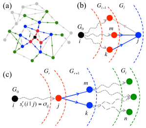
The algorithm starts from a given root $i$ and builds the $L$-range subgraph $\bm{C}_{L}$ containing all nodes which can be reached in at most $L$ steps from $i$. Only links which are part of the shortest paths starting from the root are included in $\bm{C}_{L}$. We decompose $\bm{C}_{L}$ into shells $G_{l}(i)$ containing all the nodes at shortest path distance $l$ from the root, and all incoming edges from shell $l-1$, Fig. 1a). The root itself is considered to be shell $0$ ($G_{0}(i)$).

Let $s_{l}^{r}(i|j)=\sum_{n\in G_{l}}\sigma_{in}(j)$ denote the number of shortest directed paths of length $l$ from the root through node $j$ in the $r$-th shell $j\in G_{r}(i)$, and let $s_{l}^{r}(i|j,k)=\sum_{n\in G_{l}}\sigma_{in}(j,k)$ describe the same quantity for an edge $(j,k)$ in the $r$-th shell, $(j,k)\in G_{r}(i)$. We define similar quantities for betweenness, as $b_{l}^{r}(i|j)=\sum_{n\in G_{l}}\sigma_{in}(j)/\sigma_{in}$, and $b_{l}^{r}(i|j,k)=\sum_{n\in G_{l}}\sigma_{in}(j,k)/\sigma_{in}$. Then $s_{l}(j)=\sum_{i\in V}s_{l}^{r}(i|j)$ and $b_{l}(j)=\sum_{i\in V}b_{l}^{r}(i|j)$, with similar equations for edges. In these sums $r$ is not an independent variable. Given $i$ and $j$, it is the radius of shell $G_{r}(i)$ centered on $i$ and containing $j$. One can show that the following recursions hold, (see also Fig. 1):

$$\!\!\!\!\!\!s_{l}^{l}(i|j)=\mbox{$\sum_{k}$}s_{l-1}^{l-1}(i|k)\;,\;b_{l}^{l}(i|j)=1,$$ (1)

$$\!\!\!\!\!\!s_{l}^{r+1}(i|j,k)=s_{l}^{r+1}(i|k)s_{r}^{r}(i|j)/s_{r+1}^{r+1}(i|k),$$ (2)

$$\!\!\!\!\!\!b_{l}^{r+1}(i|j,k)=b_{l}^{r+1}(i|k)s_{r}^{r}(i|j)/s_{r+1}^{r+1}(i|k),$$ (3)

$$\!\!\!\!\!\!s_{l}^{r}(i|j)=\mbox{$\sum_{k}$}s_{l}^{r+1}(i|j,k),\;b_{l}^{r}(i|j)=\mbox{$\sum_{k}$}b_{l}^{r+1}(i|j,k).$$ (4)

The steps below are repeated for $l=1,\dots,L$: 1) Build $G_{l}(i)$, using breadth-first search. 2) Calculate the $l$-centrality measures ($s_{l}^{l}(i|j)$, $b_{l}^{l}(i|j)$) of all nodes in $G_{l}(i)$. 3) Moving backwards, through $r=l-1,...,1,0$, calculate the fixed-$l$ centralities of links in $G_{r+1}(i)$ and of nodes in $G_{r}(i)$, using recursions (1-4). Finally, return to step 1) until the last shell $G_{L}(i)$ is reached. In the end, we obtained the fixed-$l$ betweenness values of all nodes and edges in $\bm{C}_{L}$. This concludes the basic algorithm, which can be modified to compute different variants of BC and SC, such as excluding endpoints. Similar recursions can also be derived for load and closeness centrality Brandes (2008); Borgatti (2005).

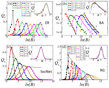
The $L$-betweenness values on large networks obey a scaling behavior as function of $L$. On Fig. 2 we plot the distribution of node betweenness values measured on the Erdős-Rényi (ER) random graph Erdős and Rényi (1960), the Barabási-Albert (BA) scale-free model Barabási and Albert (1999), the random geometric graph (RG) Dall and Christensen (2002) and the large social network (SocNet) González et al. (2008). Since in large networks $B_{L}$ grows quickly, it is better to work with the distribution $Q_{L}$ of the $\ln B_{L}$ values than with the distribution $P_{L}$ of $B_{L}$ values. However, note that $Q_{L}(\ln B)=BP_{L}(B)$. As shown on the insets of Fig. 2, the distributions $Q_{L}(\ln B)$ for different $L$ can be rescaled onto each other by plotting $Q=\sigma_{L}Q_{L}$ vs $u=[\ln(B)-\mu_{L}]/\sigma_{L}$, where $\mu_{L}$ and $\sigma_{L}$ are the mean and the standard deviation for $\ln B_{L}$. These networks were chosen to represent very different graph classes: the ER, BA and SocNet have small diameters, while the RG has no shortcuts. The RG is spatially embedded ($d=2$) unlike ER and BA; the SocNet, however, is influenced by the spatial embedding of people’s motility González et al. (2008). While BA has a power-law degree distribution $P(k)\sim k^{-3}$, both ER and RG have a Poissonian for $P(k)$, and the SocNet’s $P(k)$ resembles a log-normal Seshadri et al. (2008); Onnela et al. (2007). Both RG and SocNet have high clustering, unlike the others.

Figure 2: Distribution $Q_{L}$ of $L$-betweeness for different values of $L$. a) ER, $N=5\times 10^{4}$, $\langle k\rangle=4$, diameter $D=16$, b) BA, $N=5\times 10^{4}$, $m=3$, $D=8$, c) SocNet, $N=5,568,785$, $M=26,822,764$ and the distributions are fitted by a lognormal (black dashed curves), d) RG, $N=10^{4}$, $\langle k\rangle=15$, $D=79$. The insets show the rescaled distributions, see text.

Next we show that the scaling behavior observed for range-limited centralities in large graphs is a consequence of the scaling for shell sizes shown to exist for e.g., in random graphs with arbitrary degree distributions Newman et al. (2001); Shao et al. (2009). Here we present arguments for undirected, uncorrelated graphs and only deal with BC, extensions to other centralities mentioned above being straightforward. Let us define $\langle\cdot\rangle$ as an average over all root nodes $i$ in the graph. If $z_{l}(i)$ denotes the number of nodes on shell $G_{l}(i)$, then we model the growth of shell sizes by a branching-like process $z_{l+1}(i)=z_{l}(i)\alpha_{l}\big{[}1+\epsilon_{l}(i)\big{]}$, where $\alpha_{l}=\langle z_{l+1}\rangle/\langle z_{l}\rangle$ is the branching factor at an $l$-th shell, and $\epsilon_{l}(i)$ is a per-node, shell occupancy noise term, $|\epsilon_{l}|\ll 1$, considered to obey $\langle\epsilon_{l}(i)\rangle=0$ and $\langle\epsilon_{l}(i)\epsilon_{m}(i)\rangle=2A_{l}\delta_{l,m}$, with $A_{l}$ decreasing with $l$, supported by numerical evidence.

Figure 3: a) $b_{l}$ (circles) and $B_{l}$ (stars) vs. $l$ for some node $j$ in SocNet (red) and ER (blue). b) same as a) for RG for two arbitrary nodes $i$ and $j$. $B_{L+1}$ vs. $B_{L}$ for c) SocNet and d) RG. Each dot corresponds to a node. Ranking by BC vs $L$ for the top $10$ nodes in e) SocNet and f) RG (from Fig 4).

For undirected paths we can write $b_{l+1}(j)=(1/2)\sum_{i\in V}b_{l+1}(i|j)=z_{l+1}(j)+(1/2)\sum_{m=1}^{l}\sum_{i\in G_{m}(j)}b_{l+1}^{m}(i|j)\equiv z_{l+1}(j)+(1/2)u_{l+1}(j)$, where we used the fact that in undirected graphs $i\in G_{m}(j)\Leftrightarrow j\in G_{m}(i)$. Note that the number of terms in the inner sum $\sum_{i\in G_{m}(j)}b_{l+1}^{m}(i|j)$ is $z_{m}(j)$, which is rapidly increasing with $m$, and thus $u_{l+1}(j)$ is expected to have a weak dependence on $j$. Accordingly, we may approximate $u_{l+1}(j)\simeq\sum_{m=1}^{l}\sum_{i\in G_{m}(j)}v^{m}_{l+1}(i)$, where $v^{m}_{l+1}(i)$ is an average betweenness computed on a shell of radius $m$, centered on node $i$ : $v^{m}_{l+1}(i)=\big{[}\sum_{k\in G_{m}(i)}b_{l+1}^{m}(i|k)\big{]}/z_{m}(i)$. Based on the observation that $\sum_{k\in G_{m}(i)}b_{l}^{m}(i|k)=z_{l}(i)$, we can write that $v^{m}_{l+1}(i)\simeq z_{l+1}(i)/z_{m}(i)$. Using the recursion defined above for $z_{l+1}(i)$ as a branching process, and neglecting the small noise term, we obtain that $u_{l+1}(j)\simeq\alpha_{l}\sum_{m=1}^{l}\sum_{i\in G_{m}(j)}z_{l}(i)/z_{m}(i)$. This allows us to write a recursion for $b_{l+1}(j)$ as $b_{l+1}(j)\simeq\alpha_{l}[b_{l}(j)+z_{l}(j)/2+z_{l}(j)\epsilon_{l}(j)]$, which can be iterated down to $l=1$, where $b_{1}(j)=z_{1}(j)=k_{j}$ is the degree of $j$:

$$b_{l}(j)\simeq\beta_{l}k_{j}e^{\xi_{l}(j)}\;,$$ (5)

with $\beta_{l}=\frac{l+1}{2}\prod_{m=1}^{l-1}\alpha_{m}=\frac{l+1}{2}\langle z_{l}\rangle/\langle k\rangle$, and $\xi_{l}(j)=\sum_{n=1}^{l-1}\!\frac{l+1-n}{l+1}\;\epsilon_{n}(j)$. Eq (5) allows to relate the statistics of fixed-$l$ betweenness to the statistics of shell occupancies. Since the noise term (calculated from per-node occupancy deviations on a shell) is independent on root degree, the distribution of fixed-$l$ betweenness can be expressed as:

$$\rho_{l}(b)=\frac{1}{b}\int_{1}^{N-1}\!\!\!\!\!\!\!dk\;P(k)\Phi_{l}(\ln b-\ln\beta_{l}-\ln k)\;,$$ (6)

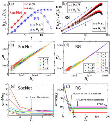
where $P(k)$ is the degree distribution and $\Phi_{l}(\xi)$ is the distribution for the noise $\xi_{l}(j)$, peaked at $\xi=0$, with fast decaying tails and $\Phi_{1}(x)=\delta(x)$. From (6) follows that the natural scaling variable for betweenness distribution is $u=\ln b-\ln\beta_{l}$. An extra $l$-dependence comes from the noise through the width $\sigma_{l}$ of $\Phi_{l}$ (for $l>1$), which can be easily accounted for by the rescaling $u\mapsto u/\sigma_{l}$, $\rho_{l}\mapsto\rho_{l}\sigma_{l}$, collapsing the distributions for different $l$-values onto the same functional form. As $\Phi_{l}$ is sharply peaked around 0, the most significant contribution to the integral (6) for a given $b$ comes from degrees $k\simeq b/\beta_{l}$. Since $k\geq 1$, we have a rapid decay of $\rho_{l}(b)$ in the range $b<\beta_{l}$, a maximum at $\overline{b}=\beta_{l}\overline{k}$ where $\overline{k}$ is the degree at which $P(k)$ is maximum, and a sharp decay for $b>(N-1)\beta_{l}$. In many networks, shell-size grows exponentially (ER, AB, and also in the SocNet), that is $\alpha_{l}\simeq\alpha=\langle z_{2}\rangle/\langle k\rangle$, until $l$ reaches the average shortest path distance. This implies that $\beta_{l}\sim\alpha^{l}$ and $b_{l}$ grows exponentially with $l$ (Fig. 3a). In this case, since $b_{l}$ is rapidly increasing with $l$, the cumulative $B_{L}(j)=\sum_{l}b_{l}(j)$ will be dominated by the largest $l$ values and thus, $B_{L}$ obeys a similar scaling supporting the observations in Fig. 2. For pure scale-free networks $P(k)=ck^{-\gamma}$, and $\rho_{l}(b)\propto(b/\beta_{l})^{1-\gamma}$ for $l>1$. In networks where the shell size grows as a power law (spatially embedded networks without shortcuts), such as RG, roadways, etc., $\beta_{l}\sim l^{d}$, where $d$ is the embedding dimension, $b_{l}(j)\sim l^{d}$ and $B_{L}\sim l^{d+1}$ (Fig.3.b).

As the contributions of the noise terms $\epsilon_{l}(j)$ to $\xi_{l}(j)$ coming from larger shells are decreasing with increasing $l$ (their weight decreases as $(l+1)^{-1}$ in addition to the decreasing of their magnitude $|\epsilon_{l}(j)|$) the $\xi_{l}(j)$ quantities rapidly converge to a constant. From (5), for a pair of nodes $i,j$: $\ln[b_{l}(i)/b_{l}(j)]=\ln(k_{i}/k_{j})+\xi_{l}(i)-\xi_{l}(j)$ showing that their relative ranking by $l$-betweenness freezes with increasing $l$. Consequently, $B_{L}$ and $B_{L+1}$ become more correlated with increasing $L$ (Fig3c,d) and the ranking of the nodes by their BC also freezes (Fig.3e,f), allowing early prediction of top betweenness nodes. Spatially embedded networks (RG) without shortcuts represent the worst case, but relative to their diameter the convergence of ranking is still fast (Fig.3f).

Figure 4: Vulnerability backbone in a RG graph ($N=5\times 10^{3}$, $\langle k\rangle=5$) for a) $L=5$, b) $L=15$, c) $L=45$, d) $L=D=195$. Darker red indicates nodes with higher $B_{L}$. In agreement with Fig.3f, VB is already well approximated at $L=45$, c).

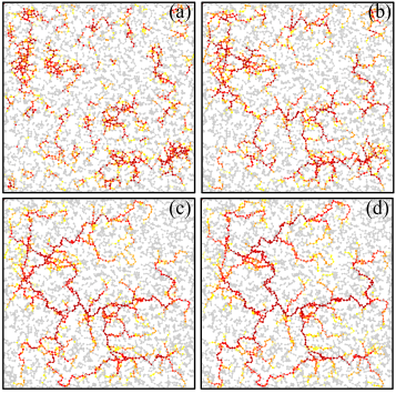
An important application of top betweenness predictability is determining the “vulnerability backbone” (VB) of a graph (crucial for network defense purposes Holme et al. (2002); DallAsta et al. (2006)) which is made by the smallest fraction of highest betweenness nodes forming a percolating cluster through the network. Fig.4 for RG (worst case) shows that the VB (red subgraph) can accurately be predicted already from $L=45$ betweenness values (Fig.4c) compared to the diameter ($D=195)$ based full betwennesses (Fig.4d).

Finally, we note that the scaling behavior can be used to provide a lower bound $L^{*}$ of the diameter, from observing that finite size effects appear when the sum of average shell sizes hits $N$: $\sum_{l=1}^{L^{*}}\langle z_{l}\rangle=\sum_{l=1}^{L^{*}}\frac{2}{l+1}\beta_{l}\langle k\rangle\simeq N$. This allows to find $L^{*}$ from the scaling behavior of $\beta_{l}$. In particular, for the SocNet $L^{*}=10$.

In summary, we have shown that the contributions to centrality measures coming from different length scales of the geodesics exhibit characteristic scaling in large graphs. Exploiting this universal property with the methods presented here makes it possible to predict betweenness values, distributions and ranking with relatively low computational costs.

This project was supported in part by the NSF BCS-0826958, HDTRA 201473-35045 and by the Army Research Laboratory, W911NF-09-2-0053. Views and conclusions are those of the authors, not representing those of the ARL or U.S. Govt.

References

- Wasserman and Faust (1994) S. Wasserman and K. Faust, Social Network Analysis: methods and applications (Cambridge Univ. Press, 1994).
- Scott (1991) J. Scott, Social Network Analysis: A Handbook (Sage Publications, 1991).
- Sabidussi (1966) G. Sabidussi, Psychometrika 31, 581 (1966).
- Friedkin (1991) N. E. Friedkin, Amer. J. of Soc. 96, 1478 (1991).
- Borgatti and Everett (2006) S. P. Borgatti and M. G. Everett, Soc. Netw. 28, 466 (2006).
- Freeman (1977) L. C. Freeman, Sociometry 40, 35 (1977).
- Borgatti (2005) S. P. Borgatti, Soc. Netw. 27, 55 (2005).
- Anthonisse (1971) J. M. Anthonisse, Tech. Rep. BN 9/71, Stichting Math. Centr., Amsterdam (1971).
- Sreenivasan et al. (2002) S. Sreenivasan et al., Phys. Rev. E 75, 036105 (2007).
- Dall’Asta et al. (2006) L. Dall’Asta et al., Theor. Comp. Sci. 355, 6 (2006).
- Dall’Asta et al. (2005) L. Dall’Asta et al., Phys. Rev. E 71, 036135 (2005).
- Goh et al. (2002) K.-I. Goh et al., Phys. Rev. Lett. 87, 278701 (2001).
- Danila et al. (2002) B. Danila et al., Phys. Rev. E 74, 046114 (2006).
- Guimera et al. (2002) R. Guimerà et al., Phys. Rev. Lett. 89, 248701 (2001).
- Holme et al. (2002) P. Holme et al., Phys. Rev. E 65, 056109 (2002).
- Motter (2002) A.E. Motter, Phys. Rev. Lett. 93, 098701 (2004).
- Vespignani (2002) A. Vespignani, Science 325, 425 (2009).
- DallAsta et al. (2006) L. Dall’Asta et al., J.Stat.Mech., P04006, (2006).
- Brandes (2001) U. Brandes, J. of Math. Sociology 25, 163 (2001).
- Newman (2001) M. E. J. Newman, Phys. Rev. E 64, 016132 (2001).
- Brandes (2008) U. Brandes, Soc. Netw. 30, 136 (2008).
- Noh,Rieger (2008) J.D. Noh and H. Rieger, Phys. Rev. Lett. 92, 118701 (2004).
- Brandes and Pich (2007) U. Brandes and C. Pich, I. J. Bif. Chaos 17, 2303 (2007).
- Geisberger et al. (2008) R. Geisberger et al., in ALENEX , 90 (2008).
- González et al. (2008) M. C. González et al., Nature 453, 779 (2008).
- Erdős and Rényi (1960) P. Erdős and A. Rényi, Publ. Math. Inst. Hung. Acad. Sci 5, 17 (1960).
- Barabási and Albert (1999) A. L. Barabási and R. Albert, Science 286, 509 (1999).
- Dall and Christensen (2002) J. Dall and M. Christensen, Phys. Rev. E 66, 016121 (2002).
- Newman et al. (2001) M. E. J. Newman et al., Phys. Rev. E 64, 026118 (2001).
- Shao et al. (2009) J. Shao et al., Phys. Rev. E 80, 036105 (2009).
- Onnela et al. (2007) J. P. Onnela et al., PNAS, 104, 7332 (2007).
- Seshadri et al. (2008) M. Seshadri et al., SIGKDD-08 (2008).