Simple Vortex States in Films of Type-I Ginzburg-Landau Superconductor

Abstract

Sufficiently thin films of type-I superconductor in a perpendicular magnetic field exhibit a triangular vortex lattice, while thick films develop an intermediate state. To elucidate what happens between these two regimes, precise numerical calculations have been made within Ginzburg-Landau theory at $\kappa=0.5$ and 0.25 for a variety of vortex lattice structures with one flux quantum per unit cell. The phase diagram in the space of mean induction and film thickness includes a narrow wedge in which a square lattice is stable, surrounded by the domain of stability of the triangular lattice at thinner films/lower fields and, on the other side, rectangular lattices with continuously varying aspect ratio. The vortex lattice has an anomalously small shear modulus within and close to the square lattice phase.

I Introduction

Thin films of a bulk type-I superconductor subject to a perpendicular magnetic field can behave like bulk type-II superconductors, in that they develop a vortex lattice. The pioneering theoretical treatments in the area, by TinkhamTinkham (1963) and MakiMaki (1965) applied Ginzburg-Landau (GL) theory in the vicinity of the critical field where the order parameter vanishes. Pearl’sPearl (1964, 1965) treatment of isolated vortices within London theory, appropriate in the low-field limit, shows that vortices in a sufficiently thin film have a long-range repulsion. This repulsion should lead to the development of a triangular vortex lattice at small fields, and it was shown by LasherLasher (1967) that a triangular vortex lattice is also favored near the upper critical field for sufficiently thin films.

On the other hand, sufficiently thick films of type-I superconductors exhibit the intermediate state. How does the magnetic flux structure evolve from triangular vortex lattice to intermediate state with increasing film thickness? In other words, what is the equilibrium phase diagram for magnetic flux structures, as a function of film thickness and magnetic field? In real superconductors the picture will necessarily be complicated by disorder and anisotropy, but the question is interesting enough within GL theory. LasherLasher (1967) was the first to address it. He showed that, within linearized GL theory, between the triangular vortex lattice and the intermediate state there were a large number of distinct vortex phases, with the triangular lattice first replaced by a square vortex lattice. Some years later CallawayCallaway (1992) pointed out that Lasher had not considered the most general Abrikosov-type solutions to the linearized first GL equation, and he carried out a comprehensive analysis of periodic vortex arrays, valid close to the upper critical field.

While theoretical analyses of the magnetic flux structure phase diagram have been restricted to the highest possible fields, interesting experimental results have appeared at very low fields. Hasegawa et al.Hasegawa et al. (1991) applied electron holography to examine the magnetic field in the space above flux structures in Pb films. They found evidence for vortices with more than one flux quantum (which they denoted MQF-A) as well as flux structures that seemed more likely to be associated with normal regions of finite cross-section (which they denoted MQF-B). “Multiply-quantized” (also known as “giant”) vortices are known to arise in various circumstances. Holes in a superconductor parallel to the field trap vortices with greater fluxoid number as their radii increase;Mkrtchyan and Shmidt (1972) the repulsion of vortices from a film edge can lead to the formation of a equilibrium giant vortex in the center of a small, thin disk;Schweigert et al. (1998) metastable giant vortices develop in field-cooling of small cylinders.Moshchalkov et al. (1997) None of these seem relevant to the experiment of Hasegawa et al., and the search for stable lattices of multiply-quantized vortex in the phase diagram for type-I films was one of the motivations for the present work.

The magnetic flux structure phase diagram is also of fundamental interest, because vortices in a film with GL parameter $\kappa<1/\sqrt{2}$ comprise an archetypical system with competing interactions. It is not obvious whether the vortex structures found by Lasher and Callaway at intermediate thicknesses survive on reducing the magnetic field, and attempts to experimentally observe such structures would benefit from theoretical guidance.

It is also noteworthy that a bulk GL superconductor with $\kappa=1/\sqrt{2}$ and at the critical field exhibits massive (in fact complete) degeneracy with respect to vortex configurations.Bogomolnyi (1976) Luk’yanchukLukyanchuk (2001) has carried out a thorough analysis of corrections to the GL functional, together with deviations of $\kappa$ and the magnetic field from their critical values, in breaking the degeneracy. He noted that demagnetization effects also break the degeneracy, but did no calculations along those lines. A film geometry corresponds to maximum demagnetization, so it may be interesting to compare the vortex phase diagram for films with $\kappa\approx 1/\sqrt{2}$ with the phase diagrams that follow from the analysis by Luk’yanchuk.

In this paper we take the first steps towards filling out the magnetic flux structure phase diagram for the minimal model, isotropic Ginzburg-Landau theory, of thin film type-I superconductors. The competition between various phases is delicate at the upper critical field, so accurate free-energy calculations for different flux structures are necessary. Consequently, we have followed the approach pioneered by Brandt for vortex lattices in bulkBrandt (1972) and, more recently, thin filmBrandt (2005) GL superconductors. The squared magnitude of the order parameter, the supervelocity, and the magnetic field are represented as linear combinations of appropriate basis functions. The GL equations then become a set of nonlinear equations for the coefficients, which are solved by iteration.

Sec. II describes the computational method in more detail. Brandt’s papers are quite explicit, so we may be brief, and highlight the modest changes we made to Brandt’s algorithm for thin films superconductors. The present calculations are restricted to magnetic flux structures consisting of singly-quantized vortices in periodic structures with one vortex per unit cell. We have found that the functional form chosen for the magnetic field in Ref. Brandt, 2005 limits the accuracy of the magnetic field and consequently the free energy, and we offer a correct and computationally convenient alternative. Sec. III presents the principal results of the calculations, which are based on evaluating the free energy for a large number of points in the space of vortex lattices structures, film thickness, and applied magnetic fields (or, equivalently, mean inductions). Phase diagrams, free energy densities, and vortex lattice shear moduli are given for $\kappa=0.5$ and 0.25. Other values of the GL parameter could have been considered but the calculations become significantly more challenging at smaller values of $\kappa$; and with results for just two values, some trends with variation of $\kappa$ may be deduced. Sec. IV offers various decompositions of the free energy density to facilitate the physical interpretation of the flux structure phase diagram. In Sec. V we summarize the results and note their limitations, indicate some directions for future theoretical work, and offer suggestions for experiments.

II Computational Method

In order to avoid unnecessary repetition of material presented in Ref. Brandt, 2005, we will start by presenting only as much of it needed to make our further developments intelligible.

The standard reduced units are employed, in which lengths are in units of the penetration depth $\lambda$, energy densities are in units of $\mu_{0}H_{c}^{2}$ (with $H_{c}$ the thermodynamic critical field) and magnetic induction is in units of $\sqrt{2}\mu_{0}H_{c}$. Note that in these units the upper critical mean induction is $\kappa$. We consider infinite films with $-d/2<z<d/2$. The GL free energy can be expressed in gauge-invariant form (rather than in terms of the GL order parameter $\psi=fe^{i\varphi}$ and vector potential $\mathbf{A}$) by writing it in terms of the square of the order parameter, $\omega=f^{2}$, the supervelocity,

$$\mathbf{Q}=\mathbf{A}-\kappa^{-1}\nabla\varphi$$ (1)

and the deviation from mean induction,

$$\mathbf{b}=\mathbf{B}-\hat{z}\bar{B}$$ (2)

We let $S$ denote both the unit cell area and the unit cell itself, depending on context; for the former, $S=\bar{B}/\Phi_{0}$ with $\Phi_{0}=2\pi/\kappa$. The free energy per unit volume of superconductor referenced to the normal state is

$$F=\frac{1}{Sd}\int_{S}\mathrm{d}x\mathrm{d}y\int_{-d/2}^{d/2}\mathrm{dz}\left[-\omega+\frac{1}{2}\omega^{2}+\frac{\left|\nabla\omega\right|^{2}}{4\kappa^{2}\omega}+\omega Q^{2}+b^{2}\right]+\frac{2}{Sd}\int_{S}\mathrm{d}x\mathrm{d}y\int_{d/2}^{\infty}\mathrm{dz}[B^{2}-\bar{B}^{2}]$$ (3)

where the contribution of the first two terms in the first integral is the condensation free energy $F_{\mathrm{cond}}$, that of the next two terms is the kinetic energy of the supercurrent $F_{\mathrm{kin}}$, that of the last term is the internal field energy $F_{\mathrm{mag}}$, and that of the second integral is the stray field energy $F_{\mathrm{stray}}$. In order to determine the phase diagram we will compare the minimum $F$ for different vortex lattice structures with the same value of $\bar{B}$ (and hence $S$). For a particular vortex lattice structure, minimizing the GL free energy with respect to variations in the order parameter yields the first GL equation

$$\frac{1}{2\kappa^{2}}\left(\nabla^{2}\omega-\frac{\left|\nabla\omega\right|^{2}}{2\omega}\right)=-\omega+\omega^{2}+\omega Q^{2}$$ (4)

The second GL equation is

$$\nabla\times\mathbf{B}=-\omega\mathbf{Q}$$ (5)

which is identical to Ampere’s law in reduced units because the supercurrent $\mathbf{j}$ is

$$\mathbf{j}=-\omega\mathbf{Q}$$ (6)

A key step in Brandt’s approach is to decompose the supervelocity as

$$\mathbf{Q}=\mathbf{Q}_{A}+\mathbf{q}$$ (7)

where $\mathbf{Q}_{A}$ is the supervelocity of the Abrikosov solution corresponding to the given vortex lattice, which satisfies

$$\nabla\times\mathbf{Q}_{A}=\left[\bar{B}-\Phi_{0}\sum\delta_{2}\left(\mathbf{r}_{\bot}-\mathbf{R}_{\mathrm{vortex}}\right)\right]\hat{z}$$ (8)

where $\mathbf{r}_{\bot}=(x,y)$, $\delta_{2}$ is the two-dimensional Dirac delta function, and the sum runs over all vortices. Inside the film,

$$\mathbf{b}=\nabla\times\mathbf{q}$$ (9)

With these definitions and relations, the problem is to determine $\omega$, $\mathbf{q}$ and $\mathbf{b}$ that minimize the free energy. Brandt’s Ansatz for these fields is as follows:

$$\omega\left(\mathbf{r}\right)=\sum_{\mathbf{K}_{\bot},K_{z}}a_{\mathbf{K}_{\bot}K_{z}}\left[1-\cos\mathbf{K}_{\bot}\cdot\mathbf{r}_{\bot}\right]\cos\left(K_{z}z\right)$$ (10)

$$\mathbf{q}\left(\mathbf{r}\right)=\sum_{\mathbf{K}_{\bot},K_{z}}b_{\mathbf{K}_{\bot}K_{z}}\frac{\hat{z}\times\mathbf{K_{\bot}}}{K_{\bot}^{2}}\sin\mathbf{K_{\bot}}\cdot\mathbf{r_{\bot}}\cos K_{z}z$$ (11)

$$b_{z}\left(\mathbf{r}\right)=\sum_{\mathbf{K}_{\bot},K_{z}}b_{\mathbf{K}_{\bot}K_{z}}\cos\mathbf{K}_{\bot}\cdot\mathbf{r}_{\bot}\cos K_{z}z$$ (12)

$$\mathbf{b_{\bot}}\left(\mathbf{r}\right)=\sum_{\mathbf{K}_{\bot},K_{z}}b_{\mathbf{K}_{\bot}K_{z}}\frac{\mathbf{K}_{\bot}K_{z}}{\left|\mathbf{K}_{\bot}\right|^{2}}\sin\mathbf{K}_{\bot}\cdot\mathbf{r}_{\bot}\sin K_{z}z$$ (13)

Here $\mathbf{K}_{\bot}$ is the set of reciprocal lattice vectors for the vortex lattice and $K_{z}=\left(2\pi/d\right)n$ with $n$ running over the whole numbers. Several features of this Ansatz are worth noting. Only two sets of expansion coefficients, $a_{\mathbf{K}_{\bot}K_{z}}$ and $b_{\mathbf{K}_{\bot}K_{z}}$, are required because $\mathbf{b}$ and $\mathbf{q}$ are linked by (9). The periodicity of the $\omega$ combined with the quadratic behavior of $\omega$ near the vortices suggests the form of expansion for the $\mathbf{r}_{\bot}$ dependence in (10), while the boundary condition for the order parameter at a superconductor-insulator interface makes the cosine expansion natural for the $z$ dependence. Eq. (11) leads to supercurrents with, as one would anticipate, only in-plane components, as well as with the appropriate periodicity and behavior near vortex lines. The motivation for the $z$ dependence of the expansions for $\mathbf{b}$ and $\mathbf{q}$ is that $\mathbf{q}$ and $b_{z}$ are even functions of $z$ while $\mathbf{b_{\bot}}$ is an odd function.

Inserting (10) and (11) into the first GL equation and applying orthogonality of trigonometric functions leads to coupled nonlinear equations for the expansion coefficients $a_{\mathbf{K}_{\bot}K_{z}}$ and $b_{\mathbf{K}_{\bot}K_{z}}$ which can be readily cast in the form of equations for the $a_{\mathbf{K}_{\bot}K_{z}}$ suitable for solution by iteration: see Eq. (21) below. More equations must come from the second GL equation inside the film, together with $\nabla\times\mathbf{b}=0$ outside the film and the boundary conditions on the induction. The induction above the film satisfies

$$B_{z}=\bar{B}+\sum_{\mathbf{K}_{\bot}}b_{\mathbf{K_{\bot}}}^{\mathrm{s}}\cos\mathbf{K}_{\bot}\cdot\mathbf{r}_{\bot}e^{-K_{\perp}(z-d/2)}$$ (14)

$$\mathbf{B}_{\perp}=\sum_{\mathbf{K}_{\bot}}b_{\mathbf{K_{\bot}}}^{\mathrm{s}}\frac{\mathbf{K}_{\bot}}{K_{\perp}}\sin\mathbf{K}_{\bot}\cdot\mathbf{r}_{\bot}e^{-K_{\perp}(z-d/2)}$$ (15)

and the continuity-of-$B_{z}$ boundary condition may be expressed as

$$b_{\mathbf{K_{\bot}}}^{\mathrm{s}}=\sum_{K_{z}}b_{\mathbf{K}_{\bot}K_{z}}\cos dK_{z}/2$$ (16)

It is convenient to derive the equations for the expansion coefficients by direct minimization of the free energy (including the stray field energy) with respect to the $b_{\mathbf{K}_{\bot}K_{z}}$, which leads to Eqs. (19) through (23) of Ref. Brandt, 2005, which we will not reproduce here.

In order to carry out a calculation of the expansion coefficients it is necessary to truncate the expansion, setting $a_{\mathbf{K}_{\bot}K_{z}}$ and $b_{\mathbf{K}_{\bot}K_{z}}$ to zero for $\mathbf{K}_{\bot}K_{z}$ outside some range. It is also necessary to approximate the integrals that appear in the iteration equations as finite sums. Those integrals arise from applying orthogonality relations and, ideally, the coefficient truncation and numerical integration could be done consistently, so that the trigonometric functions retained in the expansion are orthogonal with respect to the numerical integration. This is done naturally for the $z$ coordinates of the integration, by making the simplest choice of uniform spacing. In the $xy$ plane Brandt employs a rectangular grid for integration but a circular domain for the allowed $\mathbf{K}_{\bot}$ values. Though a rectilinear domain for $\mathbf{K}_{\bot}$ would be more consistent we have followed Brandt’s choice, on the grounds that when $K_{\perp}$ is large the expansion coefficients ought to be small.

What is there to object to in the method described above? In brief, Eq. (11) (and its corollaries Eqs. (12) and (13)) impose periodic boundary conditions in the $z$ direction which are not physically appropriate. According to (13), as the film surface is approached from within, $\mathbf{b_{\bot}}\left(\mathbf{r}\right)\rightarrow 0$. This leads to a discontinuity in $\mathbf{b_{\bot}}$ across the film boundary, as can be seen from Eq. (15), and that discontinuity implies a surface current which does not exist.

The consequences of this flaw in the Ansatz are surprisingly difficult to see—no clear sign of it appears in the results presented by Brandt in Ref. Brandt, 2005, many of which we reproduced independently. When we implemented that method the first suggestion of a problem came when we compared two calculations of the supercurrent which should have given the same results, namely $\mathbf{j}=-\omega\mathbf{Q}$ and $\mathbf{j}=\nabla\times\mathbf{B}=\nabla\times\mathbf{b}$. An example is shown in Fig. 1, for a system at fairly low mean induction. Note that the supercurrent calculated according to $\nabla\times\mathbf{B}$ actually circulates in the wrong direction for some values of $z$. A hint that the problem was the form of the $z$ dependence in Eqs. (11)–(13), and not simply an error in our implementation as we first supposed, was that the disagreement become more evident as the maximum value of $K_{z}$ was increased.

Our solution is to replace the cosine expansion for the $z$-dependence of $\mathbf{q}$ with an expansion in terms of Legendre polynomials of even order. Instead of Eqs. (11)–(13), take

$$\mathbf{q}\left(\mathbf{r}\right)=\sum_{\mathbf{K_{\bot}},l}b_{\mathbf{K_{\bot}}l}\frac{\hat{z}\times\mathbf{K_{\bot}}}{K_{\bot}^{2}}\sin\mathbf{K_{\bot}}\cdot\mathbf{r_{\bot}}P_{2l}\left(2z/d\right)$$ (17)

$$b_{z}\left(\mathbf{r}\right)=\sum_{\mathbf{K_{\bot}},l}b_{\mathbf{K_{\bot}}l}\cos\mathbf{K_{\bot}}\cdot\mathbf{r_{\bot}}P_{2l}\left(2z/d\right)$$ (18)

$$\mathbf{b}_{\bot}\left(\mathbf{r}\right)=\sum_{\mathbf{K_{\bot}},l}b_{\mathbf{K_{\bot}}l}\frac{-\mathbf{K_{\bot}}}{K_{\bot}^{2}}\sin\mathbf{K_{\bot}}\cdot\mathbf{r_{\bot}}\frac{2}{d}P^{\prime}_{2l}\left(2z/d\right)$$ (19)

There is an additional benefit of the Legendre polynomial expansion for the accuracy of the calculations. A numerical scheme for $z$-integration which maintains orthogonality of the Legendre polynomials is appropriate for the iterative calculation of the $b$ coefficients, namely, Gauss-Legendre quadrature. The abscissas for Gauss-Legendre quadrature are at zeros of $P_{n}$ (where $n$ is larger than the highest order used in the Ansatz), and these zeros are more numerous near the film surfaces where the most rapid changes occur for $\mathbf{b}$ and $\mathbf{q}$.

We now present the full scheme for generating solutions to the GL equations for films. We use $\langle\cdots\rangle_{\mathrm{U}}$ to denote the volume average over a unit cell by numerical quadrature in which the $z$ abscissas are uniformly spaced, while $\langle\cdots\rangle_{\mathrm{G}}$ is the same, except it employs Gauss-Legendre quadrature for the $z$ coordinate. Angle brackets without a subscript refers to an analytic expression for the volume average over the unit cell. Before beginning the iterative calculations a set of initial $a_{\mathbf{K}_{\bot}K_{z}}$ and $b_{\mathbf{K}_{\perp}l}$ coefficients must be chosen; we will discuss that choice following the iteration scheme.

For the order parameter coefficients we use Brandt’s iteration scheme, without modification, but for completeness we include it here. Defining

$$g=|\nabla\omega|^{2}/4\kappa^{2}\omega$$ (20)

the first GL equation leads to the iteration

$$a_{\mathbf{K}_{\bot}K_{z}}:=\frac{4\langle(\omega^{2}-2\omega+\omega Q^{2}+g)\cos\mathbf{K_{\bot}\cdot r_{\bot}}\cos K_{z}z\rangle_{\mathrm{U}}}{(\delta_{K_{z},0}+1)((K_{\perp}^{2}+K_{z}^{2})/2\kappa^{2}+1)}$$ (21)

This is always followed by an iteration to minimize $F$ by multiplying all the $a_{\mathbf{K}_{\bot}K_{z}}$ by the same factor,

$$a_{\mathbf{K}_{\bot}K_{z}}:=a_{\mathbf{K}_{\bot}K_{z}}\langle\omega-g-\omega Q^{2}\rangle_{\mathrm{U}}/\langle\omega^{2}\rangle_{\mathrm{U}}$$ (22)

This step was introduced by Brandt in solving the GL equations in bulk superconductors; if omitted, the calculations generally do not converge.

Next comes the iteration for the $b_{\mathbf{K}_{\perp}l}$ . Our modification of the expansions for $\mathbf{b}$ and $\mathbf{q}$ require corresponding changes to the iteration scheme compared to Ref. Brandt, 2005. It is convenient to construct some auxiliary quantities such as the stray-field expansion coefficients

$$b_{\mathbf{K_{\bot}}}^{\mathrm{s}}=\sum_{l}b_{\mathbf{K_{\bot}}l}$$ (23)

(compare Ref. Brandt, 2005 Eqs. (10) and (21)); a quantity that arises from $\partial\langle\omega Q^{2}\rangle/\partial b_{\mathbf{K_{\bot}}l}$,

$$D_{\mathbf{K_{\bot}}l}=\left\langle\omega\left[Q_{y}K_{x}-Q_{x}K_{y}\right]\sin\mathbf{K_{\bot}\cdot r_{\bot}}P_{2l}\left(2z/d\right)\right\rangle_{\mathrm{G}}$$ (24)

(compare Ref. Brandt, 2005 Eqs. (20) and (22)); and

$$S_{\mathbf{K_{\bot}}l}=\sum_{l^{\prime}=0}^{l}b_{\mathbf{K_{\bot}}l^{\prime}}2l^{\prime}\left(2l^{\prime}+1\right)+\sum_{l^{\prime}=l+1}b_{\mathbf{K_{\bot}}l^{\prime}}2l\left(2l+1\right)$$ (25)

which appears in

$$\partial\langle b^{2}\rangle/\partial b_{\mathbf{K_{\bot}}l}=2S_{\mathbf{K_{\bot}}l}/(dK_{\perp})^{2}+b_{\mathbf{K_{\bot}}l}/(4l+1)$$ (26)

These last two expressions are rather more complicated than the corresponding Eq. (19) of Ref. Brandt, 2005 because, unlike sines and cosines, the $P_{2l}$ and $P^{\prime}_{2l}$ are not mutually orthogonal. The second sum in Eq. (25) is finite on account of the truncation of the expansion.

With these definitions the revised iteration scheme is

$$b_{\mathbf{K_{\bot}}l}:=\frac{-2S_{\mathbf{K_{\bot}}l}-2D_{\mathbf{K_{\bot}}l}-2K_{\bot}b_{\mathbf{K_{\bot}}}^{\mathrm{s}}/d+c\left\langle\omega\right\rangle b_{\mathbf{K_{\bot}}l}}{K_{\perp}^{2}/(4l+1)+c\left\langle\omega\right\rangle}$$ (27)

where the constant $c$ and the order parameter mean $\left\langle\omega\right\rangle=\sum_{\mathbf{K_{\bot}}}a_{\mathbf{K_{\bot}}0}$ are included to stabilize the iterations (compare Ref. Brandt, 2005 Eq. (23)).

The algorithm is started with an initial guess for the $a_{\mathbf{K}_{\bot}K_{z}}$ and $b_{\mathbf{K_{\bot}}l}$ coefficients. Convergence to the physical solutions is not guaranteed, and in fact it is essential to have good initial values. We have used bulk solutionsBrandt (1997) as initial values for $a_{\mathbf{K}_{\bot}0}$ and $b_{\mathbf{K_{\bot}}0}$, with the other coefficients initially zero. One repeatedly cycles through Eqs. (21), (22), and (27) until $F$ has converged to an absolute tolerance of $1\times 10^{-10}$ or better, which typically requires about 200 iterations. This is slower convergence than is achieved with the cosine Ansatz for the $z$ dependence for the supervelocity. A possibly related matter is that we have not found a suitable expression for the “mixing parameter” $c$ that works well—large enough to maintain stability of the iteration scheme, small enough to allow for reasonably quick convergence—over the entire range of parameters that we have studied. What we do instead is to adjust $c$ during the iteration cycle by monitoring the evolution of $F_{\mathrm{mag}}$ and $F_{\mathrm{stray}}$. We have found when either of those field energies increases excessively it is a sign that an instability is developing. A scheme that works reliably is that when either $F_{\mathrm{mag}}$ and $F_{\mathrm{stray}}$ increases by more than 50% following (27) then $c$ is multiplied by 10 and the $b$-iteration is re-run; independently, every 30 iterations $c$ is divided by 2.

Although our calculations do not converge as rapidly as those reported in Ref. Brandt, 2005 they always lead to solutions with lower free energies, typically by 0.5% or less (with the same number of coefficients included in both calculations). These small differences are enough to produce noticeable changes in the phase boundaries. Our calculations also have the appealing feature that increasing the $l$ cutoff for the $b_{\mathbf{K_{\bot}}l}$ always gives an improved solution; the same is not true of increasing the $K_{z}$ cutoff for the $b_{\mathbf{K_{\bot}}K_{z}}$. Repeating the calculations presented in Fig. 1 yields supercurrent densities from $-\omega\mathbf{Q}$ and $\nabla\times\mathbf{B}$ which are nearly coincident, and which are close to the $-\omega\mathbf{Q}$ values displayed in that figure.

All of the results presented in the following sections are for calculations at $\kappa=0.5$ and 0.25; even with just those two values for the GL parameter some trends with decreasing $\kappa$ are evident. Calculations at small $\kappa$ are considerably more challenging: we have not yet been able to obtained converged solutions at $\kappa=0.1$.

III Phase Diagrams and Physical Properties

We have carried out a series of calculations at various values of $\bar{B}$ and $d$, and for several kinds of vortex lattices including triangular, square, rectangular (at various aspect ratios) and two classes of oblique lattices which we will refer to as rhombohedral (which interpolate between triangular and square at fixed unit cell area, maintaining equality of the primitive vector lengths) and sheared-triangular (which interpolate between triangular and rectangular at fixed unit cell area, keeping one primitive vector fixed). The common feature of the structures considered is that they have one vortex per unit cell, and consequently the coefficients in the expansion of the order parameter (10) are known for a bulk system just below the upper critical field.Brandt (1969) The vortex structure with lowest free energy turns out to be either triangular, square, or rectangular.

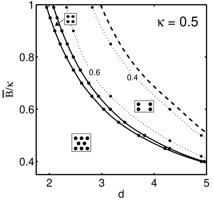
Figure 2: Vortex lattice phase diagram for $\kappa=0.5$. The triangular-square transition is discontinuous while the square-rectangular transition is continuous. Inside the rectangular phase, the dotted lines labeled 0.6 and 0.4 are contours of constant aspect ratio. The dashed line corresponds to the aspect ratio of 0.36, which is the smallest aspect ratio for which a rectangular lattice is stable at the upper critical field ($\bar{B}/\kappa=1$), following Callaway.Callaway (1992)

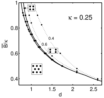
Figure 3: Same as Fig. 2, but for $\kappa=0.25$. Note the critical endpoint for the square-rectangular transition at $d\approx 2.1$.

Figs. 2 and 3 show the resulting phase diagrams for $\kappa=0.5$ and 0.25. The phases found at the upper critical field extend to lower fields, but with the phase boundaries shifting to larger thicknesses as $\bar{B}$ is reduced. At sufficiently low $\bar{B}$ the interval of thickness where the square lattice is stable is seen to vanish on the $\kappa=0.25$ phase diagram; and the same almost certainly holds for $\kappa=0.5$, but at a lower value of $\bar{B}$ than we have considered. Contours of constant aspect ratio within the rectangular phase are shown as dotted lines. On the $\kappa=0.5$ phase diagram we have included a dashed line where we speculate that the rectangular phase ends and more complicated structures with more than one flux quantum per unit cell begin; in drawing that line we are assuming that the aspect ratio within the rectangular phase is constant at the boundary with the adjacent phase.

Within linearized GL theory $d\bar{B}^{1/2}$ is constant on every phase boundary.Lasher (1967) That is not a terrible approximation, but the numerical results are noticeably different, with the domain of stability of the triangular phase reduced compared to the linearized GL theory. The critical endpoint for the square to rectangular transition is a qualitative feature that only emerges from the full GL treatment.

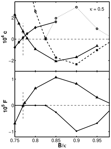
Figure 4: Shear moduli and free energies per unit volume for triangular, square, and rectangular lattices, at $\kappa=0.5$ and $d=2.4$, for mean inductions around the domain of stability of the square lattice. Free energies are referenced to value for the square lattice; on that graph the triangular lattice values are the triangles and the minimum-$F$ rectangular lattice values are the circles. The vertical dashed segments in both plots indicate the transition between triangular and square lattices, to make clear the discontinuity in shear modulus. On the shear modulus plot, triangles are $c_{66}$ for the triangular lattice, diamonds are $c_{66}$ for the square lattice, squares are $\frac{1}{2}(c_{11}-c_{12})$ for the square lattice, and circles are $\frac{1}{2}((c_{11}+c_{22})/2-c_{12})$ for the minimum-$F$ rectangular lattice. Both $F$ and $c$ are in units of $\mu_{0}H_{C}^{2}$.

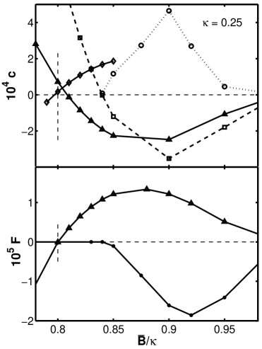
Figure 5: Same as Fig. 4, but for $\kappa=0.25$ and $d=0.94$.

It is of interest to look at the free energies that underlie the phase diagrams, to see the scale of the free energy differences. In the lower panel of Fig. 4, $F$ is presented as a function of mean induction for $\kappa=0.5$ and $d=2.4$, while Fig. 5 does the same for $\kappa=0.25$ and $d=0.94$ (the latter thickness is chosen so that the phase transitions in the two figures are at roughly the same values of $\bar{B}/\kappa$). The rhombohedral lattice free energies, not shown in those figures, are nearly degenerate with the free energies of square and triangular lattices at phase transition between them, and close to the transition their free energies almost linearly interpolate between square and triangular lattice free energies.

Shear moduli have been evaluated for the three lattice structures which appear on the phase diagram: see the upper panels of Figs. 4 and 5. For triangular lattices the only shear modulus is $c_{66}=\frac{1}{2}(c_{11}-c_{12})$. For square lattices there are two distinct types of shear, with moduli $c_{66}$ and $\frac{1}{2}(c_{11}-c_{12})$: the former preserves equality of primitive lattice vector length, while the latter preserves orthogonality of primitive lattice vectors. We present both on the figures because the latter vanishes at the continuous square-rectangular transition and the former is anomalously small at the discontinuous triangular-square transition. For the rectangular lattices we considered only the shear mode which preserves orthogonality of primitive lattice vectors; the corresponding modulus is $\frac{1}{2}((c_{11}+c_{22})/2-c_{12})$. In every case the shear modulus is calculated by evaluating the energy difference between the reference lattice structure and a slightly sheared lattice. One can see in the figures the small domains of metastability for the triangular and square lattice phases. It is also apparent that the vortex lattices at these values of $\kappa$ and $d$ are anomalously soft for a wide range of mean inductions.

IV Free Energy Decompositions

The preceding section presented the main physical results of the calculations, but further insight might be gained by comparing not just $F$ for different lattice structures but also various “components” of the free energy.

One decomposition is into the condensation, kinetic, and magnetic terms described following Eq. (3). Let us first consider $\kappa=0.5$, $\bar{B}/\kappa=0.825$, and $d=2.0$, which is in the triangular phase but not far from the square phase. For a bulk system at the same GL parameter and mean induction, the square lattice has lower free energy density than the triangular lattice. Why is the relative stability reversed? In Table 1 we present the differences in free energy density components between the film and the bulk system for both triangular and square vortex lattices. The signs of all those differences may be understood as a consequence of suppression of the order parameter in the film compared to the bulk. However, the exchange of stability is a more subtle matter, since that depends on the difference (triangular minus square lattice values) of those free energy density differences. Alternatively, we can compare the triangular and square lattice free energy density components for films of different thickness, as presented in Table 2. It is then evident that with increasing thickness, the transition to the square vortex lattice is favored only by the condensation term.

We can also examine the $z$-dependence of the free energy density, integrating in Eq. (3) only over $x$ and $y$ and dividing only by $S$ to define $F(z)$. ($F_{\mathrm{stray}}$ is taken as a $z$-independent contribution to $F(z)$.) Figure 6 compares square and triangular vortex lattices for $\kappa=0.5$ just below the upper critical field for $d=1.5$, 2.0, and 2.5. The triangular lattice has lower total free energy only for $d=1.5$. However, in every case $F(z)$ is lower for the triangular lattice when $z\approx d/2$, and, with decreasing $z$, $F(z)$ decreases more rapidly for the square lattice than for the triangular lattice. Figure 6 is thus consistent with the interior of the film being more bulk-like than the surface; and in fact $F(0)$ approaches $F$ for a bulk system with as $d$ increases. In terms of the free energy components, the condensation term is nearly independent of $z$, as is $\omega$ (as pointed out by Brandt for films of type-II superconductorsBrandt (2005)). The kinetic term is responsible for the $z$-dependence seen in Figure 6, since the magnetic term is smaller at the surface, where the field lines spread out, than in the center of the film.

V Conclusions

We have improved Brandt’s methodBrandt (2005) for solving the GL equations for thin-film superconductors in perpendicular magnetic fields, and applied it to a series of calculations for various vortex lattice structures with one vortex per primitive cell in type-I superconductor films of intermediate thickness ($d\sim\lambda$). The phase diagrams presented in Sec. (III) are the first step beyond the linearized theory towards the development of an accurate equilibrium flux structure phase diagram for films of type-I GL superconductors. The results suggest that non-triangular flux lattice structures (square and rectangular) may arise at mean inductions well below the upper critical value. For future work we wish to carry out similar calculations for flux structures with more that one vortex per primitive cell, as well as lattices of multiply-quantized vortices and various intermediate state models; these will require different expansions for the in-plane variation of $\omega$, $\mathbf{q}$ and $\mathbf{b}$ but Legendre function expansions for the $z$ dependence should still be applicable.

The anomalous softness of the vortex lattice in and near the domain of stability for the square vortex lattice offers hope that some features of the theoretical phase diagram might be observed in critical current measurements, in the form of a “peak effect”Pippard (1969) well below the upper critical field. However, quantitative comparison between the theoretical phase diagrams and experimental results will necessarily be complicated by anisotropy and, possibly, thermal fluctuations.Hove et al. (2002)

Figure 1: Supercurrent density components $j_{x}$ and $j_{y}$ calculated from $-\omega\mathbf{Q}$ (crosses) and $\nabla\times\mathbf{B}$ (circles) from solutions by the method of Ref. Brandt, 2005 for a system with $\kappa=0.5$, $\bar{B}=0.4/\kappa$, $d=4.3$, and a $32\times 13\times 9$ grid for real-space sampling. The vortex lattice is triangular, with one primitive translation being $x_{1}\hat{x}$. In these plots $y=0.017x_{1}$, with $z=0.89d/2$ for (a) and (b) and $z=0$ for (c) and (d).

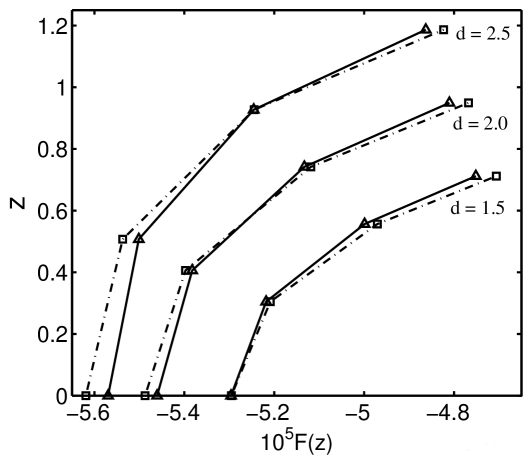
Figure 6: Free energy density dependence on $z$ for films of various thickness with $\kappa=0.5$ and $\bar{B}=0.99/\kappa$, for square and triangular vortex lattices (indicated by the squares and triangles, lines are guides for the eye).

Table 1: Film minus bulk free energy density terms for $\kappa=0.5$, $\bar{B}/\kappa=0.825$, and $d=2.0$.

	$\mathrm{Triangular}$	$\mathrm{Square}$
$10^{4}\,\Delta F_{\mathrm{cond}}$	$161.$	$180.$
$10^{4}\,\Delta F_{\mathrm{kin}}$	$-116.$	$-129.$
$10^{4}(\Delta F_{\mathrm{mag}}+\Delta F_{\mathrm{stray}})$	$-25.5$	$-29.0$

Table 2: Differences in free energy density terms (triangular lattice minus square lattice) at $\kappa=0.5$ and $\bar{B}/\kappa=0.825$ for several values of $d$. Note that $\Delta F<0$ for $d=2.0$ but is positive at the other thicknesses.

$d$	$2.0$	$2.33$	$2.6$
$10^{4}\,\Delta F_{\mathrm{cond}}$	$-4.44$	$-2.64$	$-1.37$
$10^{4}\,\Delta F_{\mathrm{kin}}$	$6.55$	$5.29$	$4.42$
$10^{4}(\Delta F_{\mathrm{mag}}+\Delta F_{\mathrm{stray}})$	$-2.31$	$-2.60$	$-2.81$