Detailed Classification of Swift’s Gamma-Ray Bursts

Abstract

Earlier classification analyses found three types of gamma-ray bursts (short, long and intermediate in duration) in the BATSE sample. Recent works have shown that these three groups are also present in the RHESSI and the BeppoSaX databases. The duration distribution analysis of the bursts observed by the Swift satellite also favors the three-component model. In this paper, we extend the analysis of the Swift data with spectral information. We show, using the spectral hardness and the duration simultaneously, that the maximum likelihood method favors the three-component against the two-component model. The likelihood also shows that a fourth component is not needed.

1 Introduction

Decades ago Mazets et al. (1981) and Norris et al. (1984) suggested that there might be a separation in the duration distribution of gamma-ray bursts (GRBs). Kouveliotou et al. (1993) found bimodality in the distribution of the logarithms of the durations. Today it is widely accepted that the physics of these two groups (short and long bursts — called also as Type I and Type II classes (Zhang et al., 2007; Kann et al., 2008; Zhang et al., 2009; Lü et al., 2010)) — are different, and these two kinds of GRBs are different phenomena (Norris et al., 2001; Balázs et al., 2003; Fox et al., 2005; Kann et al., 2008). The angular sky distribution of the short BATSE’s GRBs is anisotropic (Vavrek et al., 2008). In the Swift database (Sakamoto et al., 2008), the measured redshift distributions for the two groups are also different: for short bursts the median is 0.4 (O’Shaughnessy et al., 2008) and for the long ones it is 2.4 (Bagoly et al., 2006).

In the Third BATSE Catalog (Meegan et al., 1996) — using uni- and multi-variate analyses — Horváth (1998) and Mukherjee et al. (1998) found a third type of GRBs. Later several papers (Hakkila et al., 2000; Balastegui et al., 2001; Rajaniemi & Mähönen, 2002; Horváth, 2002; Hakkila et al., 2003; Horváth et al., 2004; Borgonovo, 2004; Horváth et al., 2006; Chattopadhyay et al., 2007) confirmed the existence of this third ("intermediate" in duration) group in the same database. The celestial distribution of this third group in the BATSE sample is also anisotropic (Mészáros et al., 2000a, b; Litvin et al., 2001; Magliocchetti et al., 2003; Vavrek et al., 2008).

Recent works analyzed the Swift (Horváth et al., 2008; Huja et al., 2009), RHESSI (Řípa et al., 2008, 2009) and BeppoSaX (Horváth, 2009) data, respectively. They have found the intermediate class in all the three satellites’ data: in the Swift database the one-dimensional maximum likelihood (ML) analysis of the durations has proven the existence of these three subgroups (Horváth et al., 2008); a preliminary study by the same method of the BeppoSAX database (Frontera et al., 2009) gave support for this class (Horváth, 2009); in the RHESSI database two methods led to the same results - the same one-dimensional ML method of the durations and the bivariate ML method using both duration and hardness (Řípa et al., 2008, 2009).

A method to infer the physical origin of GRBs was developed recently (Zhang et al., 2007; Kann et al., 2008; Zhang et al., 2009). Many other observed parameters besides duration are used as the differentiation criteria. Such a scheme only result in two major types of GRBs (Type I and Type II). On the other hand, GRBs may be classified using different parameters other than duration (e.g., Lü et al. (2010)). We shall discuss these more in the discussion section.

Horváth et al. (2006) analyzed the BATSE data using duration and hardness simultaneously; Řípa et al. (2009) studied the RHESSI data with the same configuration. The bivariate analysis on the Swift database has not been done yet. Horváth et al. (2008) only provided the one-dimensional analysis of the durations.

Hence, to get a complete picture, one has to analyze the Swift data also - using both the duration and hardness simultaneously - with the bivariate ML method. This is the aim of this paper.

The paper is organized as follows. Section 2 briefly summarizes the method of the two-dimensional fits, Section 3 defines the sample, Section 4 deals with these fits in the two-dimensional parameter space and confirms the reality of the intermediate group, Section 5 discusses the physical differences between the classes, Section 6 contains the discussion and Section 7 summarizes the conclusions of this paper.

2 The mathematics of the method

When studying a GRB distribution, one can assume that the observed probability distribution in the parameter space is a superposition of the distributions characterizing the different types of bursts present in the sample. Using the notations $x$ and $y$ for the variables (in a two-dimensional space) and using the law of full probabilities (Rényi, 1962), one can write

$$p(x,y)=\sum\limits_{l=1}^{k}p(x,y|l)p_{l}.$$ (1)

In this equation, $p(x,y|l)$ is the conditional probability density assuming that a burst belongs to the $l$th class. $p_{l}$ is the probability for this class in the observed sample ($\sum\limits_{l=1}^{k}p_{l}=1$), where $k$ is the number of classes. In order to decompose the observed probability distribution $p(x,y)$ into the superposition of different classes, we need the functional form of $p(x,y|l)$. The probability distribution of the logarithm of durations can be well fitted by Gaussian distributions, if we restrict ourselves to the short and long GRBs (Horváth, 1998). We assume the same also for the $y$ coordinate. With this assumption we obtain, for a certain $l$-th class of GRBs,

$$p(x,y|l)=\frac{1}{2\pi\sigma_{x}\sigma_{y}\sqrt{1-r^{2}}}\times\;\;\;\;\;\;\;\;\;\;\;\;\;\;\;\;\;\;\;\;\;\;\;\;\;\;\;\;\;\;\;\;$$

$$\exp\left[-\frac{1}{2(1-r^{2})}\left(\frac{(x-a_{x})^{2}}{\sigma_{x}^{2}}+\frac{(y-a_{y})^{2}}{\sigma_{y}^{2}}-\frac{2r(x-a_{x})(y-a_{y})}{\sigma_{x}\sigma_{y}}\right)\right],\;$$ (2)

where $a_{x}$, $a_{y}$ are the means, $\sigma_{x}$, $\sigma_{y}$ are the dispersions, and $r$ is the correlation coefficient (Trumpler & Weaver, 1953). Hence, a certain class is defined by five independent parameters, $a_{x}$, $a_{y}$, $\sigma_{x}$, $\sigma_{y}$, and $r$, which are different for different $l$. If we have $k$ classes, then we have $(6k-1)$ independent parameters (constants), because any class is given by the five parameters of Eq.(2) and the weight $p_{l}$ of the class. One weight is not independent, because $\sum\limits_{l=1}^{k}p_{l}=1$. The sum of $k$ functions defined by Eq.(2) gives the theoretical function of the fit.

Figure 1: Distribution of $N=325$ GRBs in the $\{\lg T_{90};\lg HR\}$ plane.

By decomposing $p(x,y)$ into the superposition of $p(x,y|l)$ conditional probabilities one divides the original population of GRBs into $k$ groups. Decomposing the left-hand side of Eq.(1) into the sum of the right-hand side, one needs the functional form of $p(x,y|l)$ distributions, and also $k$ has to be fixed. Because we assume that the functional form is a bivariate Gaussian distribution (see Eq.(2)), our task is reduced to evaluating its parameters, $k$ and $p_{l}$.

Balázs et al. (2003) used this method for $k=2$, and gave a more detailed description of the procedure. However, that paper used fluence instead of hardness, and used the BATSE data. Also Horváth et al. (2006) used this method analyzing the BATSE data. Here we will make similar calculations for $k=2$, $k=3$ and $k=4$ using Swift observations.

3 The sample

In the Swift BAT Catalog (Sakamoto et al., 2008) there are 237 GRBs, of which 222 have duration information. Following the same procedure of data reduction we have extended this sample with all the bursts detected until mid 2008 December (ending with GRB 081211a). Our total sample thus comprises the first four years of the Swift satellite (since the detection of its first burst GRB 041217) and includes $325$ bursts. $222$ from Sakamoto et al. (2008) and $103$ reduced by us. The data reduction was done by using HEAsoft v.6.3.2 and calibration database v.20070924. For light curves and spectra we ran the batgrbproduct pipeline We fitted the spectra integrated for the duration of the burst with a power-law model and a power-law model with an exponential cutoff. As in Sakamoto et al. (2008) we have chosen the cutoff power-law model if the $\chi^{2}$ of the fit improved by more than 6.

For calculating the hardness ratio, we have chosen fluence 2 ($25-50keV$) and fluence 3 ($50-100keV$) and the hardness is defined by the $HR=F3/F2$ ratio. Figure 1 shows the distribution of GRBs in the $\{\lg T_{90};\lg HR\}$ plane, where the fits were made for $x=\lg T_{90}$ and $y=\lg HR$.

4 Bivariate ML fitting

In order to find the unknown constants in Eq.(2), we use the maximum likelihood (ML) procedure of parameter estimation (Balázs et al., 2003). Assuming a set of $N$ observed $[x_{i},y_{i}],\,(i=1,\dots,N)$ values ($N$ is the number of GRBs in the sample for our case, which here is 325) we can define the likelihood function in the usual way, after fixing the value of $k$, in the form

$$L=\sum\limits_{i=1}^{N}\ln p(x_{i},y_{i})\;,$$ (3)

where $p(x_{i},y_{i})$ has the form given by Eq.(1). Similarly to what was done by Balázs et al. (2003) and Horváth et al. (2006), the EM (Expectation and Maximization) algorithm is used to obtain the $a_{x},a_{y},\sigma_{x},\sigma_{y},r$, and $p_{l}$ parameters at which $L$ reaches its maximum value. We made the calculations for different values of $k$ in order to see the improvement of $L$, as we increase the number of parameters to be estimated. Tables 1-2 summarize the results of the fits for $k=2$ and $k=3$. Figures 2 and 3 show the results in the $\{\lg T_{90};\lg HR\}$ plane.

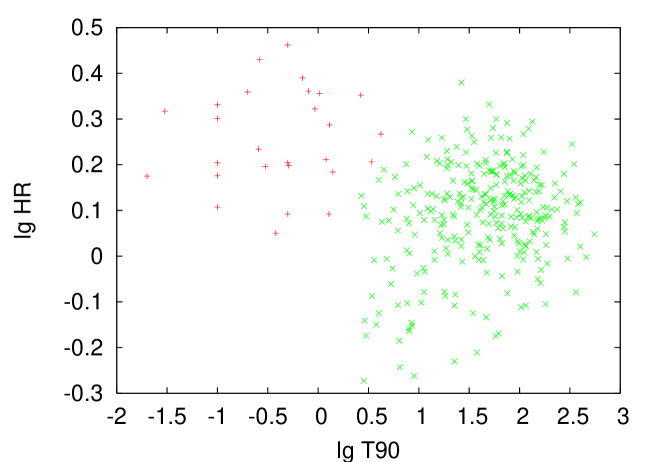
Figure 2: Distribution of $N=325$ GRBs in the $\{\lg T_{90};\lg HR\}$ plane. The different symbols mark bursts belonging to the short (red +) and long (green x) classes, respectively.

Table 1: Results of the EM algorithm in the $\{\lg T_{90};\lg HR\}$ plane. $k=2$   

$l$	$p_{l}$	$a_{x}$	$a_{y}$	$\sigma_{x}$	$\sigma_{y}$	$r$
1	0.082	-0.383	0.256	0.602	0.114	0.071
2	0.918	1.628	0.096	0.516	0.117	0.226

The confidence interval of the estimated parameters can be given on the basis of the following theorem. Denoting by $L_{max}$ and $L_{0}$ the values of the likelihood function at the maximum and at the true value of the parameters, respectively, one can write asymptotically as the sample size $N\rightarrow\infty$ (Kendall & Stuart, 1983),

$$2(L_{max}-L_{0})\approx\chi_{m}^{2}$$ (4)

where $m$ is the number of estimated parameters ($m=6k-1$ in our case), and $\chi_{m}^{2}$ is the usual $m$-dimensional $\chi^{2}$ function (Trumpler & Weaver, 1953). Moving from $k=2$ to $k=3$ the number of parameters $m$ increases by 6 (from 11 to 17) and $L_{max}$ grows from 506.6 to 531.4. Since $\chi_{17}^{2}=\chi_{11}^{2}+\chi_{6}^{2}$ the increase in $L_{max}$ by a value of 25 corresponds to a value of 50 for a $\chi_{6}^{2}$ distribution. The probability for $\chi_{6}^{2}\geq 50$ is very low ($10^{-8}$), so we may conclude that the inclusion of a third class into the fitting procedure is well justified by a very high level of significance.

Moving from $k=3$ to $k=4$, however, the improvement in $L_{max}$ is 3.4 (from 531.4 to 534.8) corresponding to $\chi_{6}^{2}\geq 6.8$, which can happen by chance with a probability of 33.9 %. Hence, the inclusion of the fourth class is not justified. We may conclude from this analysis that the superposition of three Gaussian bivariate distributions - and only these three ones - can describe the observed distribution.

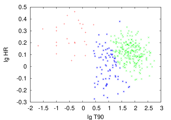
Figure 3: Distribution of $N=325$ GRBs in the $\{\lg T_{90};\lg HR\}$ plane. The different symbols mark bursts belonging to the short (red +), intermediate (blue *) and long (green x) classes, respectively.

Table 2: Results of the EM algorithm. $k=3$   

$l$	$p_{l}$	$a_{x}$	$a_{y}$	$\sigma_{x}$	$\sigma_{y}$	$r$
1	0.079	-0.426	0.259	0.576	0.114	0.120
2	0.296	1.076	0.025	0.376	0.129	-0.004
3	0.626	1.882	0.130	0.350	0.093	-0.237

This means that the 17 independent constants for $k=3$ in Table 2 define the parameters of the three groups. We see that the mean hardness of the intermediate class is very low - the third class is the softest one. This is in a good agreement with Horváth et al. (2006), who found that the intermediate duration class is the softest in the BATSE database. In that database, 11% of all GRBs belonged to this group. In our analysis, $p_{2}=0.296$; therefore, 30% of the Swift bursts belong to the third group.

5 Separation of GRBs into the classes

Based on the calculations in the previous paragraph, we resolved the $p(x,y)$ probability density of the observed quantities into a superposition of three Gaussian distributions. Using this decomposition, we can classify any observed GRB into the classes represented by these groups (this is similar to the Horváth et al. (2006) work dealing with the BATSE data). In other words, we develop a method allowing us to obtain, for any given GRB, its three membership probabilities, which define the likelihood of the GRB to belong to the short, intermediate, and long groups. The sum of these three probabilities is unity. For this purpose we define the following $I_{l}(x,y)$ indicator function, which assigns to each observed burst a membership probability in a given $l$ class as follows:

$$I_{l}(x,y)=\frac{p(x,y|l)p_{l}}{\sum\limits_{l=1}^{k}p(x,y|l)p_{l}}.$$ (5)

According to Eq.(5), each burst may belong to any of the classes with a certain probability. In this sense, one cannot assign a given burst to a given class with absolute certainty, but with a given probability. This type of classification is called a "fuzzy" classification (McLachlan & Basford, 1988). Although, any burst with a given $[x,y]$ could be assigned to all classes with a certain probability, one can select that $l$ at which the $I_{l}(x,y)$ indicator function reaches its maximum value. For $k=3$, Figure 3 shows the bursts’ distribution in the $\{\lg T_{90};\lg HR\}$ plane indicating the group memberships. For the community, we make the list of the membership probabilities available on the internet. Table 3 contains the six GRBs identified as intermediate having redshift information.

Table 3: The six intermediate GRBs identified with redshift.   

GRB id.	3rd type prob.	redshift
050525	0.78	0.606
050922C	0.71	2.17
060206	0.88	4.048
071117	0.82	1.331
080913	0.67	6.695
081007	1.00	0.5295

One can demonstrate the robustness of classification by comparing the results obtained from the $\{\lg T_{90};\lg HR\}$ and the $\{\lg T_{50};\lg HR\}$ planes. A cross tabulation between these two classifications is given in Table 4. According to the table, the short and long classes correspond within a few percent to the respective groups obtained from the other classification. We even have three zeros, which means, for example, no short burst, classified with $\{\lg T_{90};\lg HR\}$, was identified as long with the $\{\lg T_{50};\lg HR\}$ classification and since the other number is also zero, this applies vice versa. Consequently, the robustness of the short and long groups is well established. On the other hand, the population of the intermediate group is less numerous when classifying in the $\{\lg T_{50};\lg HR\}$ plane than in the other one. Table 4 clearly shows that the $\{\lg T_{90};\lg HR\}$ classification, except for three (two for long and one for short), contains all GRBs assigned to the intermediate group by $\{\lg T_{50};\lg HR\}$.

Table 4: The cross-tabulation of the two classifications (with $T_{90}-HR$ and $T_{50}-HR$).   

T50 $\backslash$ T90	short ($T_{90}-HR$)	interm. ($T_{90}-HR$)	long ($T_{90}-HR$)	total
short ($T_{50}-HR$)	24	0	0	24
interm. ($T_{50}-HR$)	1	62	2	65
long ($T_{50}-HR$)	0	24	212	236
total	25	86	214	325

The intermediate bursts classified in the $\{\lg T_{90};\lg HR\}$ plane indicated 0 GRBs from the short and 24 from the long group identified in the other plane. This moderately high number of indicated bursts clearly shows that a slight variation of the parameters of the Gaussian distribution representing the intermediate group results in a moderate change in the number of identified objects in this group. Comparing the number of GRBs belonging to the intermediate group, one gets 86 and 65; 86 are identified as intermediate with the $T_{90}$ analysis and 65 are identified as intermediate with the $T_{50}$ analysis (see the numbers in Table 4).

If one assigned the burst to that group that had the maximum membership probability, a slight change in the parameters of the corresponding Gaussian distribution may move the GRB to an other group. On the contrary, the fuzzy classification assigns membership probability to all of the bursts. Hence, a small variation of the parameter gives a small variation in the estimated number of bursts in the intermediate group obtained by summing the membership probabilities of all GRBs in the sample. There is a further issue to be considered here. The duration ($T_{90}$) is dependent on the energy range at which we are measuring. This results in a further fuzziness factor in the determination of the membership.

6 Discussion

6.1 Redshift Distributions

The cumulative redshift distribution of the three populations is shown in Figure 4. Redshifts were taken from Amati et al. (2008). Only a subset of the classified bursts had redshift information and we considered bursts where the probability of belonging to a given population is higher than $97\%$. This means $6$ short, $9$ intermediate, and $50$ long GRBs. The long and short population redshift distributions are significantly different ($99.4\%$ significance). The intermediate GRBs redshift distribution is clearly between the short and long redshift distributions, which could mean that they are further than the short bursts and closer than the long ones. However, probably owing to the small number of data points the difference is not significant. We have tried several statistical tests, such as Kolmogorov-Smirnov, Wilcoxon, and Mann-Whitney. None of them showed high significance; the best one was $92\%$. Therefore, we are not able to prove that the long and the intermediate bursts came from different redshift distributions. A more extensive analysis on these aspects as well as the afterglow properties of the intermediate group of events will be presented in a parallel work (de Ugarte Postigo et al., 2010).

Figure 4: Cumulative redshift distribution of the three classes. The continuous line is the short, the dashed line is the intermediate, and the dotted line is the long population.

6.2 The $E_{\mathrm{peak}}-E_{\mathrm{iso}}$ (Amati) Relation

Once we classify the bursts, it is also possible to investigate their properties in the context of the $E_{\mathrm{peak}}-E_{\mathrm{iso}}$ or Amati-relation (Amati et al., 2008) in the case of bursts with measured redshift. The Amati-relation (Amati et al., 2002) is a correlation between the rest-frame peak energy of the GRB spectrum ($E_{\mathrm{peak}}$) and the isotropic-equivalent energy release of the burst($E_{\mathrm{iso}}$).

Again, only a fraction of the populations had redshift and could be placed on the $E_{\mathrm{peak}}-E_{\mathrm{iso}}$ plane. We have $18$ from the long population and $6$ from the intermediate. Both groups seem to follow the same relationship. As the Amati-relation is not valid for the short population, the intermediate bursts are more closely related to the long population than to the short class.

Intermediate bursts do not populate the most energetic regime of the $E_{\mathrm{peak}}-E_{\mathrm{iso}}$ plane unlike the long bursts (see Figure 5). They tend to have lower isotropic energies compared to the long population. The small number of data points makes hard to give firm assertions at this time. Also, there is no significant clustering of intermediate bursts on this plane.

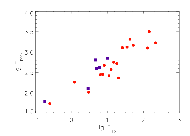
Figure 5: $E_{\mathrm{peak}}-E_{\mathrm{iso}}$ relation of the classified bursts. Red symbols represent long GRBs, and intermediate bursts are plotted in blue. The y-axis is the 10-base logarithm of $E_{\mathrm{peak}}$ in keV, and the x-axis is the 10-base logarithm of $E_{\mathrm{iso}}$ in units of $10^{52}$ erg/s.

6.3 Relation to Other Classifications

One can compare this classification to the Type I/II method put forward by Zhang et al. (2007) and Zhang et al. (2009). The Type I/II scheme looks for signatures of the binary merger and the collapsar scenario (as association with supernova, host galaxy properties, spectral lag etc.) in bursts and classifies them accordingly. Currently these two scenarios are thought to be the most probable progenitors of GRBs. This method uses a wide range of observations for classification (some deemed more decisive than others) and as such only a fraction of the bursts can be assigned Type I or II. Zhang et al. (2009) publish a table with the most certain members called the Gold sample. Though this scheme allows only for two classes it is worth checking their membership in our classification scheme.

There are five bursts of Type I in the Gold sample. GRB050709 was detected by HETE II so it is not included in our sample. The other four GRBs are listed in Table 5. This table contains the group membership probabilities of the bursts from the Type I Gold sample of Zhang et al. (2009), which clearly shows none of them belong to the intermediate class.

Table 5: Membership probabilities of the Type I Gold sample of Zhang et al. (2009) (columns 2-4). The memberships calculated without the extended emission (EE) are in the last three columns (marked with a *).

GRB name	P(short)	P(interm.)	P(long)	P∗(short)	P∗(interm)	P∗(long)
050509B	1	0	0	1	0	0
050724	0	0.02	0.98	0.02	0.95	0.03
060614	0	0.02	0.98	0.01	0.98	0.01
061006	0	0.01	0.99	0.53	0.44	0.03

The lightcurves of the last three of the bursts in Table 5 have a short-hard spike followed by an extended emission tail. If we disregard the extended emission we get a different duration. The intermediate group membership probability increases in this case to $\sim 0.95$, $0.98$ and $\sim 0.45$ for 050724, 060614 and 061006 respectively. 061006 has a $\sim 0.55$ probability of belonging to the short group. Care must be taken with these probabilities as only a whole new classification with the new durations would yield the correct membership probabilities.

GRB 060218 and X-ray flash 080109 have associated supernovae. Unfortunately, there is no duration available for any of them. For 060218, a minimum duration of $\sim 2700$ s can be established (Sakamoto, 2006), and the logarithm of hardness ratio of $\lg HR=-0.15$ can be derived. These values place this burst to the extreme right of the hardness-duration diagram and thus it belongs to the long population (though it is very soft). 080109 was detected with XRT and BAT only measured upper limits; therefore, we cannot infer anything about its group membership.

7 Conclusion

In the BATSE analysis Horváth et al. (2006) found the intermediate type of burst to be the softest. To be sure that the classifications are free of instrumental effects, it is important to compare the results obtained with datasets from different satellites. This is one of the main aims of this paper. We find that the bursts observed by Swift can be divided (in the duration hardness plane) by three groups and only three groups as happened with the BATSE sample.

Our results, summarized in Table 2, are very similar to Horváth et al. (2006) results obtained using the BATSE data. This indicates that the two satellites are observing a similar population of bursts. The relative size of the different groups will differ with the detector parameters: the Swift observations are more sensitive for soft and weak bursts; hence, the observation probability of the intermediate group members is slightly enhanced compared to BATSE (from 11% to 30% ).

An important question that must be answered in this context is whether the intermediate group of GRBs, obtained in the previous paragraph from the mathematical phenomenological classification, really represents a third type of burst physically different from both the short and the long population.

To infer the physical origin of a GRB, one must collect more direct information about the GRB progenitors. For example, most long GRBs are found to have irregular host galaxies with intense star formation (Fruchter et al., 2006) and some are associated with a supernova (Pian et al. (2006), and references therein). Some short GRBs are associated with nearby galaxies with low star formation rate (Gehrels et al., 2005; Fox et al., 2005; Berger et al., 2005; Zhang et al., 2007), which point toward a possible origin of compact star mergers.

Since one has only two main types of suggested progenitors, massive star progenitors for long (Type II) and compact star mergers for short (Type I), there are two possibilities:

A, There are only two physically different types of GRBs, and the statistically significant third group belongs to one of them.

B, The third group is physically real, and one should look more carefully at the new observations to find this new type of progenitor.

According to this paper’s analysis, the intermediate GRBs are the softest among the three classes. This different small mean hardness and also the different average duration suggest that the intermediate group should also be a different phenomenon, that is, both in hardness and in duration the third group differs from the other two.

To sum up, our bivariate ML method confirmed the existence of the third intermediate subgroup on the high significance level in the Swift database. Existence of other groups is not supported. It is conjectured that the GRBs of intermediate subgroup are physically different phenomena.

References

- Amati et al. (2002) Amati, L., et al., 2002, A&A, 390, 81
- Amati et al. (2008) Amati, L., et al., 2008, MNRAS, 391, 577
- Bagoly et al. (2006) Bagoly, Z., et al. 2006, A&A, 453, 797
- Balastegui et al. (2001) Balastegui, A., Ruiz-Lapuente, P., & Canal, R. 2001, MNRAS, 328, 283
- Balázs et al. (2003) Balázs, L.G., Bagoly, Z., Horváth, I., Mészáros, A., & Mészáros, P. 2003, A&A, 401, 129
- Berger et al. (2005) Berger, E., et al. 2005, Nature, 438, 988
- Borgonovo (2004) Borgonovo, L. 2004, A&A, 418, 487
- Chattopadhyay et al. (2007) Chattopadhyay, T., Misra, R., Chattopadhyay, A. K., & Naskar, M. 2007, ApJ, 667, 1017
- Fox et al. (2005) Fox, D.B., Frail, D.A., Price, P.A., et al. 2005, Nature, 437, 845
- Frontera et al. (2009) Frontera, F., et al. 2009, ApJS, 180, 192
- Fruchter et al. (2006) Fruchter, A.S., Levan, A.J., Strolger, L., et al. 2006, Nature, 441, 463
- Gehrels et al. (2005) Gehrels, N., Sarazin, C.L., O’Brien, P.T., et al. 2005, Nature, 437, 851
- Hakkila et al. (2000) Hakkila, J., et al. 2000, ApJ, 538, 165
- Hakkila et al. (2003) Hakkila, J., Giblin, T. W., Roiger, R. J., Haglin, D. J., Paciesas, W. S., & Meegan, C. A. 2003, ApJ, 582, 320
- Horváth (1998) Horváth, I. 1998, ApJ, 508, 757
- Horváth (2002) Horváth, I. 2002, A&A, 392, 791
- Horváth (2009) Horváth, I. 2009, Ap&SS, 323, 83
- Horváth et al. (2006) Horváth, I., Balázs, L. G., Bagoly, Z., Ryde, F., & M száros, A. 2006, A&A, 447, 23
- Horváth et al. (2008) Horváth, I., Balázs, L. G., Bagoly, Z., & Veres, P. 2008, A&A, 489, L1
- Horváth et al. (2004) Horváth, I., Mészáros, A., Balázs, L. G., & Bagoly, Z. 2004, Baltic Astronomy, 13, 217
- Huja et al. (2009) Huja, D., Mészáros, A., & Řípa, J. 2009, A&A, 504, 67
- Kann et al. (2008) Kann, D. A. et al. eprint arXiv:0804.1959
- Kendall & Stuart (1983) Kendall, M., & Stuart, A. 1983, The Advanced Theory of Statistics, Vols. 1–3 (New York: Macmillan)
- Kouveliotou et al. (1993) Kouveliotou, C., et al. 1993, ApJ, 413, L101
- Litvin et al. (2001) Litvin, V.F., Matveev, S.A., Mamedov, S.V., & Orlov, V.V. 2001, Pis’ma v Astronomicheskiy Zhurnal, 27, 416
- Lü et al. (2010) Lü, H-J., Liang, E-W., Zhang, B-B., & Zhang, B. eprint arXiv:1001.0598
- Magliocchetti et al. (2003) Magliocchetti, M., Ghirlanda, G., & Celotti, A. 2003, MNRAS, 343, 255
- Mazets et al. (1981) Mazets, E.P., et al. 1981, Ap&SS, 80, 3
- McLachlan & Basford (1988) McLachlan, G. J., & Basford, K. E. 1988, Mixture models (New York: Marcel Dekker)
- Meegan et al. (1996) Meegan C. A., et al. 1996, ApJS, 106, 65
- Mészáros et al. (2000a) Mészáros, A., Bagoly, Z., & Vavrek, R. 2000a, A&A, 354, 1
- Mészáros et al. (2000b) Mészáros, A., Bagoly, Z., Horváth, I., Balázs, L.G., & Vavrek, R. 2000b, ApJ, 539, 98
- Mukherjee et al. (1998) Mukherjee, S., et al. 1998, ApJ, 508, 314
- Norris et al. (1984) Norris, J.P., et al. 1984, Nature, 308, 434
- Norris et al. (2001) Norris, J.P., Scargle, J.D., & Bonnell, J.T. 2001, in Gamma-Ray Bursts in the Afterglow Era, Proc. Int. Workshop held in Rome, Italy, eds. E. Costa et al., ESO Astrophysics Symp. (Berlin: Springer), p. 40
- O’Shaughnessy et al. (2008) O’Shaughnessy, R., Belczynski, K., & Kalogera, V. 2008, ApJ, 675, 566
- Pian et al. (2006) Pian, E., Mazzali, P.A., Masetti, N., et al. 2006, Nature, 442, 1011
- Rajaniemi & Mähönen (2002) Rajaniemi, H.J., & Mähönen, P. 2002, ApJ, 566, 202
- Rényi (1962) Rényi, A. 1962. Wahrscheinlichtkeitsrechnung (Berlin: VEB Deutscher Verlag der Wissenschaften)
- Řípa et al. (2008) Řípa, J., et al. 2008, in AIP Conf. Proc. 1000, Gamma-Ray Bursts 2007, ed. M. Galassi, D. Palmer and E. Fenimore, (Melville, NY: AIP), 56
- Řípa et al. (2009) Řípa, J. et al. 2009, A&A, 498, 399
- Sakamoto (2006) Sakamoto, T., 2006, GCN Circ., 4822, 1
- Sakamoto et al. (2008) Sakamoto, T., Barthelmy, S. D., Barbier, L., et al. 2008, ApJS, 175, 179
- Trumpler & Weaver (1953) Trumpler, R.J., & Weaver, H. F. 1953, Statistical Astronomy (Berkeley: University of California Press)
- de Ugarte Postigo et al. (2010) de Ugarte Postigo, A., Horváth, I., Veres, P., Bagoly, Z., Balázs, L. G., Kann, D. A., Gorosabel, J., Castro-Tirado, A. J., 2010, in preparation
- Vavrek et al. (2008) Vavrek, R., Balázs, L.G., Mészáros, A., Horváth, I., & Bagoly, Z. 2008, MNRAS, 391, 1741
- Zhang et al. (2007) Zhang, B., Zhang, B.-B., Liang, E.-W., Gehrels, N., Burrows, D. N., & Mészáros, P. 2007, ApJ, 655, L25
- Zhang et al. (2009) Zhang, B., Zhang, B. B., Virgili, F. J., et al. 2009, ApJ, 703, 1696