Martin O’Loughlin^a,and Lorenzo Seri^b,
a University of Nova Gorica, Vipavska 13, 5000 Nova Gorica, Slovenia
^b SISSA, Via Beirut 3, 34151, Trieste, Italy and
INFN, Sezione di Trieste, Via Valerio 2, 34127, Trieste, Italy

We study at the classical and quantum mechanical level the time-dependent Yang-Mills theory that one obtains via the generalisation of discrete light-cone quantisation to singular homogeneous plane waves. The non-Abelian nature of this theory is known to be important for physics near the singularity, at least as far as the number of degrees of freedom is concerned. We will show that the quartic interaction is always subleading as one approaches the singularity and that close enough to $t=0$ the evolution is driven by the diverging tachyonic mass term. The evolution towards asymptotically flat space-time also reveals some surprising features.

1 Introduction

The presence of singularities in the classical solutions to the Einstein equations, or to extensions of these equations that include various additional matter fields, is by now a well-established fact, initially proven for the Einstein equations by Hawking and Penrose [1]. In general singularities are regions of space-time where there is some breakdown in our classical description of the physics. Furthermore, even if we consider a singular metric configuration corresponding to a vacuum, i.e. pure gravity with no matter, small perturbations due to the introduction of matter stress-energy or arising from quantum fluctuations of matter fields will inevitably produce divergences in the equations that describe the further evolution of the system. To make further progress in the understanding of singularities one needs some theory of quantum gravity.

String Theory is a promising candidate for a theory of quantum gravity and one of our main purposes in this paper is to show how models of singularities constructed from string theory can lead to new insights. Indeed it has been shown that string theory can “resolve” certain kinds of time-independent singularities (euclidean orbifolds [2, 3]). Cornalba and Costa [4] and Liu, Moore and Seiberg [5, 6] attempted to extend these results to singularities that display some features of a Big Bang (time-dependent orbifolds), investigating in particular whether it is possible to define a temporal evolution through a singularity. This analysis led to divergent amplitudes and furthermore the actual stability of the backgrounds used in these works was brought into question [7]. Moreover these backgrounds are almost everywhere flat, being built from Minkowski space via orbifolding, thus making them unsuitable for modelling real cosmological solutions that possess non-trivial curvature.

More recently an alternative approach to the study of cosmological singularities has been introduced by Craps, Sethi and Verlinde [8] where they carry out a Discrete Light-Cone Quantisation (DLCQ) on a type-IIA background given by a flat Minkowskian metric and a dilaton linear in time. In [9] it is conjectured that DLCQ in Minkowski space enables us to non-perturbatively describe a certain sector of string theory, singled out by fixing the light-cone momentum. The CSV generalisation of this procedure, which simply involves the addition of a linear dilaton to the Minkowski background, leads to a 1+1-dimensional SYM theory with a time-dependent coupling constant $g_{\mathrm{YM}}\sim 1/g_{\mathrm{s}}\sim e^{ct}$ that is inversely proportional to the string coupling (see also [10] for a clear review of this construction). In other relevant work, as presented in [11] and references therein, an alternative and promising approach to the resolution of cosmological singularities that uses the AdS/CFT correspondence is pursued.

As mentioned, the CSV matrix big bang is derived using a flat background. It was subsequently demonstrated in [12] that a further generalisation is possible such that the DLCQ can be applied to an entire class of metrics, the Singular Homogeneous Plane Waves (SHPWs), that are non-trivially curved and singular along a null submanifold. Furthermore, these metrics are of relevance to the physics of space-time singularities as they can be found as the Penrose Limits of a large variety of singular metrics, including the Schwarzschild black hole and the Friedmann-Robertson-Walker universe [13] (time-dependent plane-waves have also been used as backgrounds for string theory, see [14]). The final theory that one obtains is again a 1+1-dimensional SYM theory (given in equation (4) of section 2) where the coupling constant now depends on time as a power $t^{q}$ and is again inversely proportional to $g_{\mathrm{s}}$. The power $q$ may be positive or negative but for us the interesting cases correspond to $q>0$ for which the Yang-Mills coupling constant becomes small near the singularity (namely $t=0$) and blows up for large times, exactly as it does in the CSV model.

We are interested in studying the two limiting cases of $t$ close to zero and $t$ very large. It is believed that in these two limiting regions the following occur:

• near the singularity the smallness of $g_{YM}$ allows the fields (coordinates) to be non-commuting and more degrees of freedom will become available. The singularity would then be in a region where the geometry of the space time is intrinsically non-commutative. This is indeed one of the general messages of CSV [8] and in the present article we present various pieces of evidence to further support this picture in the more general context of SHPWs;

• for large times the quartic interaction term built up from the product of two commutators is forced to zero in order to contrast the growth of the time-dependent $g_{YM}$, implying that the fields become ordinary commuting coordinates (the matrices are in the Cartan subalgebra) and the model reduces to the light-cone quantisation of string field theory in Minkowski space-time with a linear dilaton background. Again this is one of the messages of the CSV paper in for which, however, we encounter some difficulty in obtaining further support.

Our main goal in this paper is to investigate the validity of these qualitative conclusions. We will study a simple non-Abelian time-dependent theory that is suitable for modelling the 1+1-dimensional SYM theory obtained via the DLCQ of SHPWs. We discuss the relevance of the non-Abelian interaction near the singularity both at the classical and at the quantum mechanical levels and the way in which the normal (commutative) space-time physics may emerge from the non-Abelian physics that appears to be important near the singularity. Our paper readdresses some of the issues discussed in [16, 17] in particular as regards the physics of the singularity and the role of the quartic interaction term. We have some new insights into these questions found by studying a toy model that retains more of the non-Abelian physics in comparison to the one-dimensional model discussed in [16].

The contents of the paper are as follows: in Section 2 we review DLCQ on SHPWs, and we present the toy model that we are going to study; in Section 3 we perform a classical analysis of this model, discussing both analytically and numerically the way in which the non-Abelian interaction near $t=0$ can be considered as a perturbation and also making some considerations regarding the $t\rightarrow\infty$ physics. In the following section we begin a discussion of the quantum mechanics of our toy model, studying in subsection 4.1 the Lagrangian without quartic interaction. In subsections 4.2 and 4.3 we deal with the quantum generalisation of the classical perturbative analysis of section 3. We explain why the naive perturbative approach fails in certain cases and discuss the conditions for which the non-Abelian interaction can be said nonetheless to be always subleading near the singularity. The final subsection of section 4 contains a short discussion and interpretation of the quantum mechanics in the limit that $t\to\infty$. Section 5 contains a summary of the results and some conclusions.

2 DLCQ and non-Abelian Yang-Mills

The basic setup that we will be using throughout this paper is that of the DLCQ of SHPW’s as presented in [12]. Before we begin we will provide a brief summary of the relevant results of that paper.

Homogeneous Plane Waves are particular plane wave space-times that are homogeneous, meaning that they have a transitive isometry algebra [18]. The generic plane wave metric in Brinkmann coordinates is

$$ds^{2}=-2dx^{+}dx^{-}+A_{ij}(x^{+})x^{i}x^{j}(dx^{+})^{2}+(d\vec{x})^{2}.$$ (1)

This space has $2d-3$ Killing vectors corresponding to a Heisenberg algebra of $2(d-2)$ components and an extra translation Killing vector $\partial_{-}$. Homogeneous plane waves have an additional Killing vector related to a transformation in the $x^{+}$-direction. For (non-singular) homogeneous plane waves this arises when $A_{ij}(x^{+})$ is constant in which case the additional Killing vector is related to translations in $x^{+}$. Singular homogeneous plane waves instead correspond to $A_{ij}(x^{+})=B_{ij}/(x^{+})^{2}$ in which case the additional Killing vector is related to the scaling $(x^{+},x^{-})\rightarrow(\mu x^{+},\mu^{-1}x^{-})$. For SHPWs the DLCQ prescription involves three steps, each related to symmetries of the space-time. First the alignment (by a null rotational isometry) of an almost null-circle with a space-like circle, then a rescaling of all energies by a boost isometry that acts directly on $\partial_{+}$, and finally a rescaling of the coordinates (mass/length scales) as originally proposed by Seiberg and Sen [19, 20] using a homothety of the metric.

In this paper we will restrict attention to the class of SHPW metrics that arise when taking the Penrose limit of space-time singularities [13]. In Brinkmann coordinates these are

$$ds^{2}=-2dx^{+}dx^{-}+\sum_{i}\frac{p_{i}(p_{i}+2)}{4(x^{+})^{2}}(x^{i})^{2}(dx^{+})^{2}+\sum_{i}(dx^{i})^{2}.$$ (2)

We will be interested in solutions to the type IIA string theory with a dilaton of power law form,

$$\mbox{e}^{\phi}=(x^{+})^{-q},$$ (3)

as dictated by the choice of metric and equations of motion to be discussed below.

Applying the DLCQ procedure to this system of metric and dilaton one finds a two-dimensional matrix string theory described by the action,

$$S=\frac{1}{2}\int d^{2}\sigma\;\mathtt{Tr}\left(-\frac{1}{2g^{2}_{YM}(t)}\eta^{\alpha\gamma}\eta^{\beta\delta}F_{\alpha\beta}F_{\gamma\delta}-\eta^{\alpha\beta}\delta_{ij}D_{\alpha}X^{i}D_{\beta}X^{j}\right.\\ +\left.g^{2}_{YM}(t)\delta_{ik}\delta_{jl}[X^{i},X^{j}][X^{k},X^{l}]+\sum_{i}\frac{p_{i}(p_{i}+2)}{4t^{2}}(X^{i})^{2}\right)\;\;,$$ (4)

where we are in light-cone gauge $x^{+}=t$ and the coupling constant of the gauge theory is related in a simple manner to the original dilaton,

$$g_{YM}(t)\sim\frac{1}{g_{s}\ell_{s}}\mbox{e}^{-\phi}=\frac{1}{g_{s}\ell_{s}}t^{q}\;\;.$$ (5)

This construction provides us, in principle, with a non-perturbative description of the full string theory in a sector of fixed light-cone momentum. Note the simplicity of this final result. After a series of T and S-dualities on the original metric and dilaton of type IIA string theory, we find this matrix string action again containing the original type IIA metric. Note also that it is only with this choice of Brinkmann coordinates that the metric contains information free of ambiguities. A study of the same system using Rosen coordinates is likely to be fraught with interpretational difficulties due to the fact that these coordinates do not fix a unique form for the metric and thus generally contain extraneous non-geometric information.

The equations of motion of type IIA string theory give a precise relationship between the frequencies determined by the $p_{i}$ and the behaviour of the dilaton,

$$\frac{1}{4}\sum_{i}p_{i}(p_{i}+2)=2q.$$ (6)

In this paper we will consider primarily two particular relations between $p$ and $q$ although much of the analysis and conclusions are independent of these choices. Using the above equation of motion for string theory on a SHPW with d-coordinates compactified on torii and the $8-d$ remaining $p_{i}=p$ equal we find

$$q=(8-d)p(p+2)/8.$$ (7)

On the other hand, for the purpose of comparison between our results and those of [16] we also consider the case $p=2q$ which arises for type IIB D3-branes as constructed in [21].

We are only interested in the case in which $q>0$ as it is in this case that the string coupling constant diverges and the Yang-Mills coupling goes to zero like $|t|^{q}$ as the singularity at $t=0$ is approached. We see immediately that for the same range of $q$ and $|t|\rightarrow\infty$ we recover an asymptotically flat space-time with weak string coupling and a diverging Yang-Mills coupling. This means in particular that the coefficient of the quartic commutator term in the potential diverges, presumably fixing the transverse coordinates to be mutually commuting in the limit that the space-time is asymptotically (light-cone) flat. In the following we will discover that for the time-dependent system the situation is not so simple.

2.1 The toy model

To make a quantitative study of this system we will first compactify the action (4) on a world-sheet circle of radius $2\pi L$ and then expand it as a sum over the modes of the fields. Each of these modes is then described by a quantum mechanical system with a common time-dependent frequency and a quartic coupling,

$$S=\frac{1}{2}\int dt\;\mathtt{Tr}\left(\sum_{n}\dot{X}^{i\dagger}_{n}\dot{X}^{i}_{-n}-\omega_{n}(t)^{2}X^{i\dagger}_{n}X^{i}_{-n}\right.\\ \left.+\lambda\sum_{n_{1},n_{2},n_{3}}|t|^{2q}[X^{i\dagger}_{n_{1}},X_{n_{2}}^{j\dagger}][X^{k}_{n_{3}},X_{-n_{1}-n_{2}-n_{3}}^{l}]\delta_{ik}\delta_{jl}\right)$$ (8)

where the time-dependent frequency is

$$\omega_{n}(t)^{2}=\frac{n^{2}}{2\pi L}-\frac{p(p+2)}{4t^{2}}=\omega_{n}^{2}-\frac{p(p+2)}{4t^{2}}\;.$$ (9)

To reduce this still quite complicated and non-linear system to something more tractable we will consider just two $SU(2)$ matrices corresponding to two of the eight transverse coordinates and we will focus attention on a single KK mode of each coordinate with action

$$S_{\mathtt{toy}}=\frac{1}{2}\int\!dt\;\mathtt{Tr}\bigl{(}|\dot{X}|^{2}+|\dot{Y}|^{2}-\omega_{X}(t)^{2}|X|^{2}-\omega_{Y}(t)^{2}|Y|^{2}+\lambda|t|^{q}|[X,Y]|^{2}\bigr{)}$$ (10)

where

$$\omega_{X,Y}(t)^{2}=\omega_{n_{X},n_{Y}}^{2}-\frac{p(p+2)}{4t^{2}}\;.$$ (11)

We believe that this is the simplest model that retains the important features of the full non-Abelian Yang-Mills theory (compare with [16]). It has a time-dependent mass term and a time-dependent quartic potential representative of the interaction term of non-Abelian gauge theory.

Note that for the case of interest to us $q>0$ and thus the harmonic oscillator frequencies become purely imaginary as $|t|$ approaches zero. This fact will play an important role in the study of the non-Abelian physics of the singularity. This relation between gravitational singularities at strong string coupling and tachyonic behaviour in the DLCQ matrix theory is more general than that mentioned here and further discussion of this point can be found in [12].

A time-independent theory with the same Lagrangian but constant frequencies and a constant quartic coupling is well studied and it has been shown that if the energy is large with respect to the curvature of the potential then the quartic potential leads to a chaotic behaviour of the scalar fields [22]. It is further believed that if the energy is small compared to the curvature of the potential and if the quadratic term is exactly zero (as it would be for a supersymmetric system) then when the tension is taken to be very large the system is forced into a configuration consisting of commuting matrices [23].

In the limit that $t\rightarrow 0$ our non-linear problem becomes a time-dependent harmonic oscillator with a quartic perturbation. We are most interested in determining to what extent this quartic term can truly be treated as a perturbation. As the behaviour of this time-dependent system is non-trivial we will first take a look at the classical physics, both analytically and numerically. Secondly we review the quantum mechanics in the inverted time-dependent oscillator and then attempt to extend this analysis to the full quantum mechanical problem using time-dependent perturbation theory. This analysis will lead us to conclude that near the singularity the quartic non-Abelian interaction is not important whereas at infinity it plays an important role in the evolution of the system.

3 The classical physics

First of all, let us solve the classical equations for the time-dependent harmonic oscillator (taking $\lambda=0$),

$$\ddot{X}+\omega(t)^{2}X=\frac{\mathrm{d}^{2}}{\mathrm{d}t^{2}}X-\frac{p(p+2)}{4t^{2}}X+\omega^{2}X=0.$$ (12)

It is straightforward to see that one can equivalently write

$$\frac{\mathrm{d}^{2}}{\mathrm{d}t^{2}}\left(\frac{X}{\sqrt{t}}\right)+\frac{1}{t}\frac{\mathrm{d}}{\mathrm{d}t}\left(\frac{X}{\sqrt{t}}\right)+\left(\omega^{2}-\frac{(p+1)^{2}}{4t^{2}}\right)\frac{X}{\sqrt{t}}=0,$$ (13)

which is Bessel’s equation for $X/\sqrt{t}$. The solutions are,

$$X(t)=\sqrt{\omega t}\left\{aH_{\nu}(\omega t)+a^{*}H^{*}_{\nu}(\omega t)\right\},$$ (14)

where $H_{\nu}(\omega t)=J_{\nu}(\omega t)+iY_{\nu}(\omega t)$, $J_{\nu}$ and $Y_{\nu}$ are Bessel functions of the first and second kind and $\nu\equiv\frac{p+1}{2}$.

3.1 Perturbation theory

Now we rewrite our interaction term using the properties of the Pauli matrices of $SU(2)$:

$$\lambda|t|^{2q}\mathtt{Tr}|[X,Y]|^{2}=\lambda|t|^{2q}\left(|\vec{X}|^{2}||\vec{Y}|^{2}-(\vec{X}\cdot\vec{Y})^{2}\right)$$ (15)

The equations of motion are

$$\begin{split}\hat{L}(t)X_{i}+\omega_{n_{X}}^{2}X_{i}&=\lambda|t|^{2q}\left(2X_{i}|\vec{Y}|^{2}-2Y_{i}\vec{X}\cdot\vec{Y}\right),\\ \hat{L}(t)Y_{i}+\omega_{n_{Y}}^{2}Y_{i}&=\lambda|t|^{2q}\left(2Y_{i}|\vec{X}|^{2}-2X_{i}\vec{X}\cdot\vec{Y}\right),\end{split}$$ (16)

where the operator $\hat{L}(t)=-\frac{\partial^{2}}{\partial t^{2}}+\frac{p(p+2)}{4t^{2}}$. We want to study the possibility of treating the quartic term as a perturbation and so we will expand around the solutions to the time-dependent harmonic oscillator ($\lambda=0$), choosing for simplicity the initial conditions $X_{1,2}=0$ and $\dot{X}_{1,2}=0$.

For the (hopefully small) perturbations we find the linearized equations

$$\begin{split}\hat{L}(t)\delta X_{i}+\omega_{n_{X}}^{2}\delta X_{i}&=\lambda|t|^{2q}\left(2X_{i}\vec{Y}^{2}+4X_{i}\vec{Y}\cdot\delta\vec{Y}+2\vec{Y}^{2}\delta X_{i}-2Y_{i}\vec{X}\cdot\vec{Y}\right.\\ &\quad\left.-2Y_{i}\vec{X}\cdot\delta\vec{Y}-2Y_{i}\vec{Y}\cdot\delta\vec{X}-2\delta Y_{i}\vec{X}\cdot\vec{Y}\right),\\ \hat{L}(t)\delta Y_{i}+\omega_{n_{Y}}^{2}\delta Y_{i}&=\lambda|t|^{2q}\left(2Y_{i}\vec{X}^{2}+4Y_{i}\vec{X}\cdot\delta\vec{X}+2\vec{X}^{2}\delta Y_{i}-2X_{i}\vec{X}\cdot\vec{Y}\right.\\ &\quad\left.-2X_{i}\vec{Y}\cdot\delta\vec{X}-2X_{i}\vec{X}\cdot\delta\vec{Y}-2\delta X_{i}\vec{X}\cdot\vec{Y}\right).\\ \end{split}$$ (17)

Inserting the unperturbed solution and keeping only the leading terms on the rhs we then obtain,

$$\begin{split}\hat{L}(t)\delta X_{1,2}+\omega_{n_{X}}^{2}\delta X_{1,2}&=\lambda|t|^{2q}\left(-2Y_{1,2}X_{3}Y_{3}\right),\\ \hat{L}(t)\delta X_{3}+\omega_{n_{X}}^{2}\delta X_{3}&=\lambda|t|^{2q}[2X_{3}(Y_{1}^{2}+Y_{2}^{2})],\\ \hat{L}(t)\delta Y_{1,2}+\omega_{n_{Y}}^{2}\delta Y_{1,2}&=\lambda|t|^{2q}(2Y_{1,2}X_{3}^{2}),\\ \hat{L}(t)\delta Y_{3}+\omega_{n_{Y}}^{2}\delta Y_{3}&=0\end{split}$$ (18)

and we now want to specifically consider small $|t|$ where there is a possibility that the rhs of these equations is truly a perturbation to the harmonic oscillator. The generic solution to the homogeneous unperturbed equation is, to leading order,

$$\mathrm{A}t^{-\frac{p}{2}}+\mathrm{B}t^{\frac{p}{2}+1}$$

for some constants $A$ and $B$. On the rhs of our equations (17), (18) we always have the product of three solutions of this type and we can thus say that the only singular inhomogeneous term is of the form $Kt^{2q-3p/2}$. We have thus reduced our problem to that of solving (near $t=0$) equations of the general form

$$\left(\frac{\mathrm{d}^{2}}{\mathrm{d}t^{2}}-\frac{p(p+2)}{4t^{2}}\right)F(t)=Kt^{2q-3p/2}\;.$$ (19)

Using the ansatz $F(t)=Ct^{\gamma}$ we find

$$\left\{\begin{split}\gamma=&2q-\frac{3p}{2}+2,\\ C=&-\frac{K}{P(p,q)},\end{split}\right.$$ (20)

where $P(p,q)=2p^{2}+4q^{2}-6pq-5p+6q+2$. The perturbation theory is valid when $2q>p-2$ and the solution is valid provided that $P(p,q)\neq 0$. In the range of $p,q$ for which perturbation theory is valid $P(p,q)=0$ when $p=q+1/2$ and in this special case one needs to replace the above ansatz by $F(t)\sim Ct^{\gamma}log(t)$ finding

$$\left\{\begin{split}\gamma=&p/2+1,\\ C=&\frac{K}{2p+1}.\end{split}\right.$$ (21)

We are interested in the behaviour of $\delta X\sim\delta Y\sim F(t)$ as $t\to 0$ and we see for the two special cases of $q=p/2$ and $q=(8-d)p(p+2)/8$ that $F(t)$ is less singular than the unperturbed solution as a consequence of choosing $2q-p+2>0$ and $q>0$. At the moment we are implicitly considering initial conditions for which the classical particle begins its motion with $X(t_{0})$ near the origin and thus we see that its evolution is predominantly determined by the harmonic oscillator potential. In the next section we discuss the numerical integration of the full non-linear equations thus allowing us to consider initial conditions for which the quartic term is also important. We will find that after an initial transient phase as $t$ approaches the singularity the particle will once again converge to a solution determined entirely by the harmonic oscillator potential. This is one of the key messages of this article and we will return to discuss it several times in the following.

3.2 Numerical integration of the toy model

In addition to the qualitative study of these equations we were also able to carry out their numerical integration with results that largely corroborate the conclusions of the previous subsection. There are also some interesting surprises revealed by the numerical analysis related to the role of the quartic interaction in the limit that $|t|$ becomes large. Physically this is quite an interesting limit as it should tell us something about the way that string theory in an asymptotically flat space-time emerges from the non-Abelian physics near the singularity.

As we are interested in both large $|t|$, the asymptotically flat region, and small $|t|$, the singularity, we carried out numerical integration in both directions, beginning with some generic initial conditions at an intermediate value of $t$.

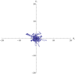
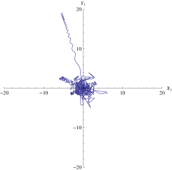
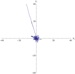
Figure 1: Numerical integration of toy model projected in the $X_{1},Y_{1}$ plane for $t_{i}=-100$ and $t_{f}=-10,-1$ and $-.001$ respectively. Note the change in scale for the third plot to allow space for the runaway behaviour at $t\rightarrow 0$.

Imposing initial conditions at a sufficiently large negative $t$ and studying the evolution as $t\rightarrow 0$ we find that the greater part of the evolution is governed by the quartic interaction term. This produces a generally oscillatory behaviour as the particle moves down into a valley where the coordinates commute until at some point, due to the steepening valley walls, the particle is forced to turn around and leave the valley, then maybe bouncing around near the origin or proceeding along another valley. Once $t$ becomes sufficiently small and $\omega_{n}(t)^{2}$ becomes negative, the corresponding coordinate crosses over from this oscillatory behaviour to a divergent tachyonic behaviour. This clearly indicates that near $t=0$, for quite generic initial conditions, the classical evolution is dominated by the quadratic $1/t^{2}$ terms in the potential, as we also concluded in the previous subsection. Figure 1 is an example of a numerical integration displaying these features.

Studying more carefully the behaviour after the appearance of negative curvature in the potential around $X=Y=0$ we see that there is a transient phase of evolution during which the particle feels the quartic interaction. The duration of this transient depends on how close the particle is to the minimum (the presence of which is a consequence of the quartic potential) but universally, at the end of this period and as $t$ gets closer to 0, the motion is dominated by the divergent quadratic potential.

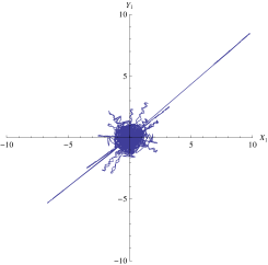
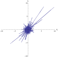
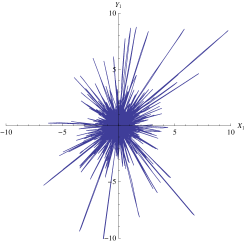
Figure 2: Numerical integration of toy model projected in the $X_{1},Y_{1}$ plane for $t_{i}=100$ and $t_{f}=500,1000$ and $5000$ respectively.

One may alternatively consider the singularity as the Penrose limit of an initial cosmological singularity and impose initial conditions at small times evolving the system to large positive times. Again, given an initial $t$ small enough so that the tachyonic mass term dominates, the evolution begins with a power law and divergent motion that then settles down to oscillations driven by the quartic interaction. Once again this term is not sufficient to restrict the matrices to commute but rather their evolution appears to be chaotic, not settling down to one direction in the Cartan subalgebra but randomly jumping from one nearly commuting configuration to another. One can clearly see this behaviour in Figure 2 where we have taken $p=0.5$ and $q=0.1$ and we begin the integration in the oscillatory region. The increasing final times $t_{f}$ illustrate the continual “chaotic” motion between various nearly commuting configurations. The long spikes represent periods during which the matrices are approximately commuting and we see that the number of excursions into different commuting valleys increases proportionally to the time elapsed. We will return to a discussion of the large $|t|$ behaviour in later sections of this paper.

Note that we have only considered the zero modes of the KK reduction to quantum mechanics. Clearly the higher modes for large enough $t$ always have a positive harmonic oscillator potential and will be bound to remain small and so the issue of commuting configurations does not arise for them.

3.3 Early times and robustness of the classical analysis: the $X^{4}$ case

In order to check the validity of our analysis we further simplify to the one-dimensional time-dependent anharmonic oscillator,

$$S=\frac{1}{2}\int dt\bigl{(}\dot{X}^{2}-\omega(t)^{2}X^{2}-\lambda|t|^{2q}X^{4}\bigr{)}.$$ (22)

Though ill-suited for modelling the behaviour of our actual theory at large times, the system given by (22) can provide us with valuable information as far as small times are concerned. Indeed we can think of the bidimensional potential $X^{2}Y^{2}$ as a special configuration of our $SU(2)$ theory (10) (namely $X\perp Y$) in which case, using the inequality $X^{2}Y^{2}\leq\frac{1}{2}(X^{4}+Y^{4})$, we see that the two decoupled copies of (22) provide us with an overestimate of the potential in this configuration.

In particular, we would like to check that

• as $t\to 0$ the solution found by including the quartic term is increasingly well approximated by that for the tachyonic $1/t^{2}$ oscillator;

• in the same limit the minimum of the potential runs off to infinity faster than the maximum possible velocity of the classical particle so that, after an initial transient evolution that depends critically on initial conditions, the particle sees only the (divergent as $t\rightarrow 0$) tachyonic mass.

Let us expand on this second point. At fixed $t$ the potential shows a minimum located at position $X_{\mathrm{min}}(t)$ that receeds to infinity as $t$ grows smaller. In order to determine if a particle can keep itself near $X_{\mathrm{min}}(t)$ during the complete evolution to $t=0$ let us set the particle mass $m=1$ and observe the following bounds on the time evolution: for fixed $t$ the maximal acceleration is seen to be

$$a_{\mathrm{max}}(t)=\frac{\sqrt{2}[p(p+2)]^{3/2}}{12\sqrt{3\lambda}}|t|^{-q-3},$$ (23)

and integrating we find (up to a constant term equal to the initial velocity) an overestimate for the speed of a particle moving in this potential,

$$v_{\mathrm{max}}(t)=-\frac{\sqrt{2}[p(p+2)]^{3/2}}{12\sqrt{3\lambda}(q+2)}|t|^{-q-2}+c.$$

On the other hand the position of the minimum is

$$X_{\mathrm{min}}(t)=\frac{1}{|t|^{q+1}}\sqrt{\frac{p(p+2)}{2\lambda}},$$ (24)

and it moves towards infinity with the speed

$$V_{\mathrm{min}}(t)=-\frac{q+1}{4}\sqrt{\frac{2p(p+2)}{\lambda}}|t|^{-q-2}.$$ (25)

The condition that for small enough $|t|$ the particle motion is not affected by the quartic term in the potential is that

$$|v_{\mathrm{max}}|<|V_{\mathrm{min}}|,$$ (26)

and thus as the two velocities have identical $t$ dependence we simply need to compare their coefficients. This leads us to the inequality

$$3\sqrt{3}(q+1)(q+2)>p(p+2),$$ (27)

and as we are assuming that $q>0$ this reduces to

$$q>\frac{1}{2}\left(-3+\sqrt{1+4\frac{p(p+2)}{3\sqrt{3}}}\right).$$ (28)

For $0<p<-1+\sqrt{1+6\sqrt{3}}$ this condition is satisfied without further restricting the range of $q$ while for $p>-1+\sqrt{1+6\sqrt{3}}$ one needs $q>-3/2+1/2\sqrt{1+4p(p+2)/3\sqrt{3}}$. When $p=2q$ or $q=(8-d)p(p+2)/8$ there is no bound on $p$ or $q$ apart from the already imposed requirement of positivity.

These general results can be easily checked in explicit examples by numerically integrating the equations of motion for $X(t)$ and choosing various initial conditions. As can be seen in figure 3 the particle after some initial transient oscillations is then quickly left behind by the minimum of the full quadratic plus quartic potential.

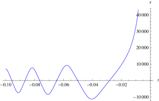
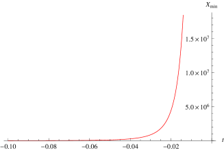
Figure 3: Numerical solution for the motion with $p=2$, $q=3$ and the particle at rest in the minimum of the potential at $t_{0}=-0.1$. The left plot is the motion of the particle and the right plot the motion of the minimum.

As a consequence of these considerations we can make the strong statement: for $t$ close (enough) to the singularity the evolution is always driven by the divergent tachyonic mass.

In section 4 we will find that much of the behaviour revealed in this classical analysis can be extended and adapted also to the quantum mechanical evolution when we “smear” the particle into a wave function.

3.4 Classical analysis: late times

Before turning to the quantum mechanics and to develop a qualitative understanding of the role of the quartic term for $|t|\to\infty$ we will perform a change of variables by multiplying the matrix coordinates by a power of $t$ so as to simplify the $t$ dependence,

$$X=t^{\gamma}W,\,\,Y=t^{\gamma}Z.$$ (29)

In addition we choose a new time parameter

$$T\sim t^{-2\gamma+1}$$

where $\gamma=-q/3$ and for $q>0$ small/large $t$ corresponds to small/large $T$.

At large $T$ the leading terms in the action of our toy model (10) become

$$S_{\mathtt{toy}}=\frac{1}{2}\!\int\!dT\,\mathtt{Tr}\left(\left|\frac{dW}{dT}\right|^{2}\right.\!\!\!+\left|\frac{dZ}{dT}\right|^{2}\!\!+m^{2}(|W|^{2}+|Z|^{2})T^{-4q/(2q+3)}\\ -\left.(4q(2q+3)-p(p+2))\frac{(|W|^{2}+|Z|^{2})}{36T^{2}}-\lambda|[W,Z]|^{2}\right).$$ (30)

$m^{2}$ in this equation contains the constant parts of the frequencies (taken to be equal for simplicity) of the two $SU(2)$ coordinates, $X$ and $Y$. Given that $q>0$ the time dependence in the $m^{2}$ term for large $T$ is subleading when compared to the quartic term but always more significant than the quadratic $1/T^{2}$ term. For large $T$ we are more interested in the behaviour of coordinates with $m^{2}=0$ as only these have the possibility of escaping to large coordinates and commuting configurations that are indicative of the emergence of string theory in flat space-time. This and related systems have been much studied in the context of hyperbolic billiards and the mixmaster universe and have been shown to be classically chaotic [24]. For large $T$ one might think that even though $W$ and $Z$ are chaotic, $X$ and $Y$ will go to zero due to the leading power of $t$ in the coordinate transformation. This is not entirely true as the chaotic dynamics implies that occasionally $W$ and $Z$ will travel a long way along one of the (infinite number of) valleys of the potential and there is no obvious limit on the magnitude of these excursions. These general considerations are in complete agreement with the large $|t|$ numerical simulation that were presented in section 3.2.

It is notable that there is no obvious way in which the quartic term is forcing the matrices to commute even though standard reasoning would lead one to such a conclusion. The coefficient of the quartic term in the toy model is indeed divergent at large $T$ indicating that energetically favoured trajectories correspond to commuting matrices. The classical evolution from strong to weak string coupling however does not force the system into such a configuration. This result presents us with two difficulties that we will revisit when we turn to the quantum mechanics of this system. The first difficulty we have is the apparent non-recovery of commuting space-time physics as one would expect for the weakly coupled string theory in an asymptotically flat space-time. The second problem is that, even if we could prove such commutativity, we still have no control over the precise direction in the configuration space where this commutativity will arise. In quantum mechanics this means that we could imagine a wave-function in which several different possibilities for commuting matrices are present but with these different possibilities not mutually commuting. At the end of the next section we will turn to look at the large $t$ quantum mechanics.

4 The quantum physics

We will now move on to the quantum mechanics and in particular to the examination of the applicability of time-dependent perturbation theory to the quartic potential as a perturbation of the time-dependent harmonic oscillator. We begin our study of the evolution of the quantum mechanical system for $|t|$ close to zero.

4.1 The time-dependent harmonic oscillator

In this first subsection we will present the solution to the time-dependent harmonic oscillator further streamlining [25] the alternative presentation in [18] rather than following the original work of Lewis and Riesenfeld [26, 27]. Recalling the solutions for the time-dependent harmonic oscillator discussed at the beginning and promoting them to solutions to the Heisenberg equations of motion for the operator $\hat{X}$ gives

$$\hat{X}(t)=\hat{a}F(t)+\hat{a}^{\dagger}F^{*}(t),$$ (31)

where

$$F(t)=\sqrt{\omega t}H_{\nu}(\omega t)$$ (32)

and the $F(t)$ are normalised such that the Wronskian $W(F,F^{*})=i$.

The time-independent operators are creation and annihilation operators and can be seen to correspond to a choice of vacuum at infinity as a consequence of the asymptotics of the Hankel function at $x\to\infty$,

$$H_{\nu}(x)\approx\sqrt{\frac{1}{2\pi x}}e^{i(x-\frac{\pi\nu}{2})}.$$

The raising and lowering operators in $\hat{X}$ are by construction time-independent and thus invariant,

$$i\frac{d\hat{a}}{dt}=0$$ (33)

naturally leading to the definition of an invariant Hermitian operator

$$\hat{I}=\hat{a}^{\dagger}\hat{a}+\frac{1}{2},$$ (34)

$$\frac{d\hat{I}}{dt}=\frac{\partial\hat{I}}{\partial t}+\frac{1}{i\hbar}[\hat{I},\hat{H}]=0.$$ (35)

Eigenvectors and eigenvalues of $\hat{I}$ are built using $\hat{a}$ and $\hat{a}^{\dagger}$ exactly as one does for the time-independent harmonic oscillator leading to

$$\begin{split}\hat{a}^{\dagger}\hat{a}|s\rangle&=s|s\rangle,\\ \hat{a}|s\rangle&=s^{\frac{1}{2}}|s-1\rangle,\\ \hat{a}^{\dagger}|s\rangle&=(s+1)^{\frac{1}{2}}|s+1\rangle.\\ \end{split}$$ (36)

The wave-function $\psi_{0}(x)=\langle x|0\rangle$ can then be found by solving the equation

$$\langle x|\hat{a}|0\rangle=0$$ (37)

and is (up to some factors of $\pi$ etc..)

$$\psi_{0}(x,t)=\frac{1}{|F|^{1/2}}e^{ix^{2}\dot{F}^{*}/2F^{*}}.$$ (38)

Using the time-independence of the oscillators and taking a partial time derivative of $\hat{a}^{\dagger}|0\rangle$ one finds that acting with the Schrödinger operator on the vacuum gives

$$(i\partial_{t}-H)|0\rangle=\varphi(t)|0\rangle.$$ (39)

To obtain an explicit expression for $\varphi(t)$ we now multiply this equation on the left by a position eigenstate $\langle x|$ and insert the above ground state wave-function. Thus

$$\varphi(t)=-\frac{i}{2|F|}\frac{d|F|}{dt}+i\frac{\dot{F}^{*}}{2F^{*}}$$ (40)

and a simple calculation gives

$$\varphi(t)=-\frac{1}{4|F|^{2}}.$$ (41)

Extending this calculation to a general eigenstate we see that

$$(i\partial_{t}-\hat{H})|s\rangle=\varphi(t)|s\rangle,$$ (42)

and as a consequence $\varphi(t)$ is independent of the state $|s\rangle$. Thus the state vectors $|\tilde{s}\rangle$ are constructed from the corresponding $|s\rangle$ as

$$|\tilde{s}\rangle=e^{-i\varphi(t)}|s\rangle.$$ (43)

The behaviour of the phase $\varphi(t)$ as $t$ approaches the origin can easily be seen to be

$$\varphi(t)\sim t^{p+1}$$ (44)

and it is straightforward to see that this phase does not exhibit any singularity at this point. However, if we happen to choose to project these eigenstates onto a position basis then one does find a singularity. Indeed

$$\psi(x,t)=\langle x,t|s\rangle=N|F|^{-1/2}\mbox{e}^{ix^{2}\dot{F}^{*}/2F^{*}}\mbox{e}^{-i\varphi(t)}H_{s}\left(\frac{x}{\hbar|F|}\right)$$ (45)

where the $H_{s}$ are Hermite polynomials. Note that this wave-function is not well defined when the singularity is approached due to the phase, proportional to $\dot{F}^{*}/F^{*}$, which changes rapidly as $t$ approaches zero [16]. On the other hand, the state vectors (43) that are solutions to the Schrödinger equation are well-behaved as $t$ approaches zero and can be continued from positive to negative $t$.

As is adequately discussed by Lewis and Riesenfeld [27] these state-vectors allow the extension of probability transitions through t=0. Thus, despite the fact that in the coordinate representation one needs to deal with diverging coordinates and rapidly varying phases there is nevertheless a way of describing evolution through the singularity. Indeed if we assume that (9) holds for all non-zero times (so that the mode has the same asymptotic frequency $\omega_{n}$ for $t\rightarrow\pm\infty$) we can choose as two independent real solutions to (12) $\sqrt{\omega_{n}t}J_{\nu}(\omega_{n}t)$ and $\sqrt{\omega_{n}t}N_{\nu}(\omega_{n}t)$ for all $t\neq 0$. In [27] it is then explained how to use these solutions to find the transition amplitude between eigenstates of the asymptottic initial and final oscillators; in our case, as the asymptotic frequencies are the same, we obtain the trivial result

$$T_{nm}=\langle n,t=\infty|m,t=-\infty\rangle=\delta_{nm}\;.$$ (46)

Defining the transition through the singularity however remains an important problem as in principle one could choose to glue modes with different asymptotic frequencies at $t=0$. In addition some extra information on the behaviour of $\hat{X}$ on both sides of the singularity is needed in order to compute the amplitudes. Finally, the extension of this discussion to QFT forces one to confront additional questions related to particle creation and the choice of vacuum. These questions will be addressed in a forthcoming publication [28].

4.2 Time-dependent perturbation theory

We will briefly look at the possibility of treating the quartic term as a perturbation by using time-dependent perturbation theory. The unperturbed states will be given by the solutions to the Schrödinger equation as provided in the previous subsection. Consider the following Hamiltonian,

$$H=H_{0}(t)+\lambda\hat{W}(t)$$ (47)

where $H_{0}(t)$ is the Hamiltonian for the time-dependent oscillator while $W(t)$ is the quartic commutator term

$$\hat{W}(t)=-|t|^{2q}\mathtt{Tr}[\hat{X},\hat{Y}]^{2}.$$ (48)

We will expand our full wave-function as a series with time-dependent coefficients

$$|t\rangle=\sum_{s}b_{s}(t)e^{i\varphi(t)}|s\rangle.$$ (49)

The requirement that this state is a solution to the full Schrödinger equation leads to the first order differential equation for $b_{s}(t)$

$$\frac{db_{s}(t)}{dt}=\frac{\lambda}{i\hbar}\sum_{s^{\prime}}\langle s|\hat{W}|s^{\prime}\rangle b_{s^{\prime}}(t).$$ (50)

To find a perturbative solution to this equation we now also expand

$$b_{s}(t)=b_{s}^{(0)}+\lambda b_{s}^{(1)}(t)+\lambda^{2}b_{s}^{(2)}(t)+\cdots$$ (51)

and retain the first non-trivial order. Specializing these general equations to our case, we have to keep in mind that the non-Abelian interaction couples six different copies of our time-dependent harmonic oscillator (with asymptotic frequencies possibly different), so if we represent the tensor product of six $\hat{I}$ eigenstates by

$$|s_{M}\rangle=|s_{X1},\dots,s_{Y1},\dots\rangle$$

and we decompose the operators $\hat{X}$ and $\hat{Y}$ then the perturbation has the general form

$$\hat{W}\sim-|t|^{2q}\sum_{i,j,l,m}F_{\omega_{X_{i}}}F_{\omega_{Y_{i}}}F_{\omega_{X_{l}}}F_{\omega_{Y_{m}}}(\delta_{il}\delta_{jm}-\delta_{ij}\delta_{lm})\times\\ \times\,(a_{X_{i}}+a_{X_{i}}^{\dagger})(a_{Y_{i}}+a_{Y_{i}}^{\dagger})(a_{X_{l}}+a_{X_{l}}^{\dagger})(a_{Y_{m}}+a_{Y_{m}}^{\dagger}).$$ (52)

The differential equation that determines $b_{s_{M}}^{(1)}(t)$ is then

$$\frac{db^{(1)}_{s_{M}}(t)}{dt}=\frac{\lambda}{i\hbar}\sum_{s_{M}^{\prime}}\langle s_{M}|\hat{W}|s_{M}^{\prime}\rangle b_{s_{M}^{\prime}}(t)$$ (53)

where the sum is performed over all combinations $s_{M}\!=\!\{s_{X1},\dots,s_{Y1},\dots\}$. To find $b^{(1)}_{s_{M}}(t)$ we need to solve a combinatorial problem and carry out an integration over $t$. For our discussion it is sufficient to consider the integration without elaborating on the details of the combinatorics

$$b^{(1)}_{s_{M}}(t)\sim\int_{-\infty}^{t}dt^{\prime}|t^{\prime}|^{2q}|F(t^{\prime})|^{4}.$$ (54)

We can investigate the convergence of this integral for $t$ near zero by expanding the Bessel functions in $|F(t)|$ around $t=0$. We find that $|F(t)|^{2}\sim|t|^{-p}$ resulting in

$$b^{(1)}_{s_{M}}(t)\sim\int^{t}|t^{\prime}|^{2(q-p)}\sim|t|^{2(q-p)+1}$$ (55)

unless $q=p-1/2$ for which case the integral has a logarithmic divergence. Thus $b^{(1)}_{s}(t)$ converges as $t\rightarrow 0$ for $2(q-p)>-1$. Going back to the two cases that we have been discussing throughout the paper we see that when $q=p(p+2)/4$ ($d=6$) we would require that $p(p-2)>-2$ which is always satisfied for $p>0$ and similarly so for other values of $d$. On the other hand, when $p=2q$ perturbation theory is only valid in the range $0<p<1$. In the next section we will investigate in greater depth the apparent breakdown of perturbation theory when $p>1$, and we will show that it is due to transient behaviour related to wave-functions that are large in the region where the quartic term becomes significant.

4.3 Evolution of wave-functions

To find the source of the problems that arose in the previous section when applying time-dependent perturbation theory to the case with $p=2q$ and $p>1$ we begin with an investigation of the time-evolution of the solutions to the Schrödinger equation in the inverted harmonic oscillator and we compare their width and the rate at which the wave-functions spread in this potential to the movement of the location of the minimum in the full oscillator plus quartic potential. We will once again simplify to a one-dimensional anharmonic oscillator (22) with the time-dependence of our DLCQ model. The action is

$$S=\frac{1}{2}\int\,dt\bigl{(}\dot{X}^{2}-\omega(t)^{2}X^{2}-\lambda|t|^{p}X^{4}\bigr{)}.$$ (56)

We will use the Ehrenfest theorem to study the general features of the evolution of the wave-function. As is well known, the Ehrenfest theorem is exact for an harmonic oscillator potential and it can easily be seen that this exactness remains when extended to a time-dependent oscillator.

Corrections to the Ehrenfest theorem may arise when the width of the wave-packet becomes comparable to the curvature of the potential as in that case one can no longer use the approximation

$$\left\langle\frac{dV(X)}{dX}\right\rangle\cong\frac{dV(\langle X\rangle)}{dX},$$ (57)

that plays an important part in the derivation of the theorem. Making a Taylor series expansion of $V(X)$ around $X=\langle X\rangle$ we can find the corrections to (57)

$$\left\langle\frac{dV(X)}{dX}\right\rangle\cong\frac{dV(\langle X\rangle)}{dX}+\frac{1}{2}\frac{d^{3}V(\langle X\rangle)}{dX^{3}}\langle(\Delta X)^{2}\rangle,$$ (58)

and it is clear that for a purely quadratic potential there are actually no such corrections. To determine the full consistency of this analysis one needs to consider that for our quartic potential the third derivative term is no longer zero. In the Heisenberg representation fluctuations of $\hat{X}$ also obey (18) and so we can say that the corrections coming from the quartic term are subleading as $t\to 0$. It is then obvious that its expectation value $\langle X\rangle$ in any state also behaves asymptotically as if there was no $X^{4}$ term in the potential. Moreover it is easy to show that for the inverse harmonic oscillator $\langle(\Delta X)^{2}\rangle$ has at most the same divergence as $\langle X\rangle^{2}$, so that the second term in the rhs of (58) is subleading: this can easily be found by solving the differential equations for the expectation values $\langle X^{2}\rangle$, $\langle P^{2}\rangle$. Thus, even if we include the cubic term to investigate corrections to the Ehrenfest theorem, we find that for $t$ sufficiently small these corrections are irrelevant.

Obviously if the initial wave-function has a significant non-zero support in the region of the quartic minimum its initial evolution will be significantly different from that of the inverted harmonic oscillator. However, by considering the behaviour of $\langle(\Delta X)^{2}\rangle$ and $\langle X\rangle^{2}$ as $t\rightarrow 0$ we conclude that after a certain period of time the wave-function no longer has significant support in the region of the minimum and its evolution is precisely that of the inverted oscillator for which the Ehrenfest Theorem applies. During this initial transient period the wave-function will have acquired a modified profile but it is guaranteed that after this period has passed the further evolution is determined precisely by the inverted harmonic oscillator potential.

To understand this evolution in a little more detail we consider $p>1$ and take a Gaussian wave-packet centred on $X=X_{0}$ as the initial condition at $t=t_{0}>0$. This wave-packet can be decomposed into a sum over the $\hat{I}$ eigenfunctions evaluated at $t=t_{0}$. This decomposition allows us to examine in detail the time evolution of the wave-packet as $t\rightarrow 0$. When the Gaussian is centred on $X_{0}<X_{\mathrm{min}}$ and its width at $t=t_{0}$ is much smaller than the distance to the minimum of the full potential we find that this wave-function spreads more slowly than the movement of the minimum (which obviously goes to $\infty$ as $t\rightarrow 0$). The same behaviour is also found for initial conditions on the Gaussian wave-packet such that its width is not necessarily small but is however less than the distance to the minimum, essentially requiring that the probability of finding the particle described by this wave-function in the minimum of the potential is very small.

The actual feasability of the numerical calculations that we performed depends in an important way on the initial conditions. Indeed we managed to carry out reliable numerical computations only for the case of a very thin initial packet centred on $x=0$, while for a more spread out initial wave-profile or one centred near the minimum of the potential a sufficiently accurate truncation of the series requires too many levels making a numerical evaluation of the evolution impractical. This notwithstanding the structure of the $\hat{I}$ eigenstates makes us confident enough to say that the spreading of all wave-functions goes roughly as $|F(t)|$ as one can immediately see from (45), namely like $t^{-\frac{p}{2}}$, while the minimum receeds to infinity like $t^{-\frac{p}{2}-1}$. The inner-product of the $\hat{I}$ eigenfunctions $\psi_{l}$ is obviously time-independent; moreover considering the integral of $\psi_{l}\psi^{*}_{l^{\prime}}$ from 0 to $\infty$ one finds that this “half product” is also finite as $t\to 0$. This means that all the states are growing more or less with the same speed, and if one of them is losing contact with the minimum, the others will lose it as well. In the previous section we found a breakdown in the naive construction of time-dependent perturbation theory for $p>1$ as a consequence of the growth with $p$ of the characteristic width of the eigenfunctions of the Schrödinger equation. We have now verified that this does not imply that given a set of initial conditions and for $t$ sufficiently close to $0$ one cannot however use time-dependent perturbation theory to describe the evolution once the transient has passed.

We have thus reached the conclusion that for $p=2q>1$ and for an arbitrary initial wave-function profile at some value $t=t_{0}$, the evolution towards the singularity will consist of an initial transient behaviour during which the non-linear effects of the quartic interaction are important, followed by an evolution for which the only important part of the potential is the purely quadratic inverted harmonic oscillator; thus even in this case, after this initial transient period, the quantum mechanics reduces to that of the time-dependent harmonic oscillator without the quartic interaction term.

4.4 $|t|\to\infty$

As mentioned at the conclusion of our discussion of the classical physics of our toy model there are some surprises in the behaviour of the system in the limit $|t|\to\infty$. These continue to be present after quantisation. A complete study of the quantum mechanics requires a deeper understanding of the evolution of the wave-function and thus a very careful numerical study of the Schrödinger equation with time-dependent mass term and time-dependent potential.

In the supersymmetric case it is believed that the effective potential is truly flat for commuting configurations [23] leading to the emergence of weakly coupled string theory in flat space-time and this should continue to be true for the time-dependent system that we are studying. For the analogous mixmaster universe, where our evolution to large $t$ corresponds mathematically to the evolution towards the mixmaster singularity, some calculations of the evolution of wave-packets have been carried out by Furusawa [29, 30] and later also by Berger [31]. Their results indicate that the system remains chaotic upon quantisation and that an initially smooth wave-function will break up into many differently localised fragments. This leads one to conclude, as we already argued in the discussion of the classical physics, that the system does not settle down into a fixed commuting configuration at late times but rather explores all different possible commuting configurations as $|t|\to\infty$.

5 Summary

As already emphasized in the introduction, the work presented in this paper was motivated by the desire to understand, in as thorough a manner as possible, the time-dependent gauge theory that one finds when the DLCQ procedure is generalised to SHPWs [12]. This time-dependent Yang-Mills theory presents interesting features arising from the interaction between time-dependent frequencies and couplings on the one hand and non-Abelian matrix fields on the other. In particular we have addressed two specific questions: To what extent is non-commutativity of the matrix fields relevant near the singularity? and: How does an intrinsically non-commutative system of matrices at $t=0$ evolve into a system of commuting coordinates as $t\rightarrow\infty$? Obviously the answers to these questions are also of interest for the study of time-dependent gauge theories independently of their matrix theory origins.

We have approached these questions at both the classical and quantum mechanical level, leaving an extension of this discussion to quantum field theory for a forthcoming paper [28]. The classical analysis revealed two interesting facts:

1. It is often said that near the singularity the non-commutativity of the non-Abelian degrees of freedom should play an important role. This is certainly true in the sense that for $|t|$ small the off-diagonal degrees of freedom are light and can easily be excited, but this does not mean that the explcitly non-Abelian quartic interaction drives the evolution. On the contrary the singular quadratic term (“divergent tachyonic mass”) eventually dominates in all cases and the non-Abelian interaction can be treated as a perturbation that is irrelevant at small times.

2. For large times the system fails to settle on a specific commuting arrangement of coordinates and appears to move randomly between different commuting configurations. In some sense the geometry can still be said to be commuting, as the coordinates spend most of their time in nearly commuting configurations and the transitions between different configurations are fast.

We began the quantum mechanical analysis with a new discussion of the solution to the time-dependent harmonic oscillator [26] anticipated in [18] and completed here. We then demonstrated that the quartic interaction is subleading as $t\to 0$ also in quantum mechanics. If one relies on the simplest analysis of perturbation theory this result appears to not hold in some of the cases that we studied but this is simply due to a non-linear transient phase of the evolution during which the interaction is not necessarily negligible. We show in generality that in all cases of interest the mass term eventually dominates the potential, a result we also anticipated in numerical calculations.

In general we have learnt that, even if the physics near the singularity is intrinsically non-Abelian as far as access to off-diagonal degrees of freedom is concerned, the non-Abelian interaction actually becomes less and less important as we approach $t=0$. What remains to be done is: the investigation of the extension of these results to quantum field theory; an analysis of the transient period during which there is also a radical change in the number of accessible degrees of freedom; and a definite interpretation of what happens at $t=0$ and as $t\rightarrow\infty$ [28].

Finally, an intriguing question that has been part of our continuing motivation for studying these matrix theories is the universality of the singularity and the simple scaling of the matrix actions under rescalings of $t$ near $t=0$. Unfortunately we do not have anything new to add to the understanding of this symmetry but we hope that our demonstration in this article of a further universal role for the divergent tachyonic masses in the near singularity region will provide additional impetus for further study of this question.

Acknowledgements

The authors would like to thank Matthias Blau and Darko Veberič for various helpful discussions.

References

- [1] S. W. Hawking and R. Penrose. The Singularities of gravitational collapse and cosmology. Proc. Roy. Soc. Lond. A314 (1970) 529.
- [2] L. J. Dixon, J. A. Harvey, C. Vafa, and E. Witten. Strings on Orbifolds. Nucl. Phys. B261 (1985) 678.
- [3] L. J. Dixon, J. A. Harvey, C. Vafa, and E. Witten. Strings on Orbifolds. 2. Nucl. Phys. B274 (1986) 285.
- [4] L. Cornalba, M. S. Costa. A new cosmological scenario in string theory Phys. Rev. D66 (2002) 066001, hep-th/0203031.
- [5] H. Liu, G. W. Moore, and N. Seiberg. Strings in a time-dependent orbifold. JHEP 0206 (2002) 045, hep-th/0204168.
- [6] H. Liu, G. W. Moore, and N. Seiberg. Strings in time-dependent orbifolds. JHEP, 0210 (2002) 031, hep-th/0206182.
- [7] G. T. Horowitz and J. Polchinski. Instability of spacelike and null orbifold singularities. Phys. Rev. D66 (2002) 103512, hep-th/0206228.
- [8] B. Craps, S. Sethi, and E. P. Verlinde. A Matrix Big Bang. JHEP, 0510 (2005) 005, hep-th/0506180.
- [9] L. Susskind. Another conjecture about M(atrix) theory. 1997, hep-th/9704080.
- [10] B. Craps. Big bang models in string theory. Class. Quant. Grav. 23 (2006) S849, hep-th/0605199.
- [11] B. Craps, T. Hertog, and N. Turok. Quantum Resolution of Cosmological Singularities using AdS/CFT. 2007, arXiv:0712.4180.
- [12] M. Blau and M. O’Loughlin. DLCQ and Plane Wave Matrix Big Bang Models. JHEP 0809 (2008) 097, arXiv:0806.3255.
- [13] M. Blau, M. Borunda, M. O’Loughlin, and G. Papadopoulos. The universality of Penrose limits near space-time singularities. JHEP 0407 (2004) 068, hep-th/0403252.
- [14] G. Papadopoulos, J. G. Russo, and A. A. Tseytlin. Solvable model of strings in a time-dependent plane-wave background. Class. Quant. Grav. 20 (2003) 969, hep-th/0211289.
- [15] Jian-Huang She, A matrix model for Misner universe JHEP 0601 (2006) 002, hep-th/0509067.
- [16] A. Awad, S. R. Das, S. Nampuri, K. Narayan, and S. P. Trivedi. Gauge Theories with Time Dependent Couplings and their Cosmological Duals. Phys. Rev. D79 (2009) 046004, arXiv:0807.1517.
- [17] B. Craps, F. De Roo, and O. Evnin. Can free strings propagate across plane wave singularities? JHEP 0903 (2009) 105, arXiv:0812.2900.
- [18] M. Blau and M. O’Loughlin, Homogeneous plane waves Nucl. Phys. B654 (2003) 135, hep-th/0212135.
- [19] N. Seiberg. Why is the matrix model correct? Phys. Rev. Lett. 79 (1997) 3577, hep-th/9710009 .
- [20] A. Sen. D0 branes on T(n) and matrix theory. Adv. Theor. Math. Phys. 2 (1998) 51, hep-th/9709220.
- [21] A. Awad, S. R. Das, K. Narayan, S. P. Trivedi, Gauge Theory Duals of Cosmological Backgrounds and their Energy Momentum Tensors. Phys. Rev. D77 (2008) 046008, arXiv:0711.2994
- [22] I. Ya. Aref’eva, A. S. Koshelev, and P. B. Medvedev. Chaos-order transition in matrix theory. Mod. Phys. Lett. A13 (1998) 2481, hep-th/9804021.
- [23] E. Witten, Bound states of strings and p-branes. Nucl. Phys. B460 (1996) 335, hep-th/9510135.
- [24] T. S. Biró. Chaos and gauge field theory. World Scientific lecture notes in physics v. 56. World Scientific, Singapore, 1994.
- [25] M. Blau and M. O’Loughlin. Notes on the time-dependent harmonic oscillator unpublished notes.
- [26] H. R. Lewis. Class of exact invariants for classical and quantum time-dependent harmonic oscillators. J. Math. Phys. 9 (1968) 1976.
- [27] H. R. Lewis and W. B. Riesenfeld. An Exact quantum theory of the time dependent harmonic oscillator and of a charged particle time dependent electromagnetic field. J. Math. Phys. 10 (1969) 1458.
- [28] M. Blau, M. O’Loughlin and L. Seri, Non-abelian QFT and space-time singularities.
- [29] T. Furusawa. Quantum Chaos of Mixmaster Universe 2. Prog. Theor. Phys. 76 (1986) 67.
- [30] T. Furusawa. Quantum Chaos of Mixmaster Universe. Prog. Theor. Phys. 75 (1986) 59.
- [31] B. K. Berger. Quantum Chaos in the Mixmaster Universe. Phys. Rev. D39 (1989) 2426.