Negative diffraction pattern dynamics in nonlinear cavities with left-handed materials

Abstract

We study a ring cavity filled with a slab of a right-handed material and a slab of a left-handed material. Both layers are assumed to be nonlinear Kerr media. First, we derive a model for the propagation of light in a left-handed material. By constructing a mean-field model, we show that the sign of diffraction can be made either positive or negative in this resonator, depending on the thicknesses of the layers. Subsequently, we demonstrate that the dynamical behavior of the modulation instability is strongly affected by the sign of the diffraction coefficient. Finally, we study the dissipative structures in this resonator and reveal the predominance of a two-dimensional up-switching process over the formation of spatially periodic structures, leading to the truncation of the homogeneous hysteresis cycle.

I Introduction

In recent years, considerable progress has been realized in the understanding of dissipative structures in spatially extended systems. The concept of dissipative structures in systems far from equilibrium has been first introduced in the context of reaction diffusion systems Glansdorff and Prigogine (1971); Turing (1952). Their formation is attributed to the balance between nonlinearities (chemical reaction or light-matter interaction), transport processes (diffusion and/or diffraction), and dissipation. Driven optical cavities filled with nonlinear media – such as Kerr materials, liquid crystals, semiconductors, or quadratic media – belong to this field of research and constitute a basic configuration in nonlinear optics. It has been shown, both experimentally and numerically, that these simple devices support stationary dissipative structures that can be either periodic or localized in space (for an overview, see Lange and Ackemann (2000); Rosanov (2002); Staliunas and Sanchez-Morcillo (2003); Mandel and Tlidi (2004); Akhmediev and Ankiewicz (2005)).

Along another line of research, theoretical and experimental studies have shown the possibility of making left-handed materials (lhm), i.e., materials with simultaneously negative permittivity and permeability. Although the early lhms were build for microwaves, the first optical lhms have been demonstrated recently Moser et al. (2005); Grigorenko et al. (2005); Alù et al. (2006); Linden et al. (2006); Feth et al. (2006); Zhang et al. (2006); Dolling et al. (2006). In his seminal work, Veselago has shown the possibility of light propagation in these materials and predicted a number of exotic effects like negative refraction, inverse Doppler shifts and radiation tension Veselago (1968). Several experiments have confirmed that lhms must be characterized by a negative index of refraction ($n<0$) and, hence, by a negative wavenumber ($k_{0}<0$) Shelby et al. (2001); Wiltshire et al. (2001). Linear optical resonators filled with lhms were shown to exhibit unique properties, most noteworthy their unconventional dispersion relation Engheta (2002). Also, periodic heterostructures that combine positive and negative refractive indexes present analogies with cavities and show interesting behavior. In particular, a new bandgap corresponding to zero averaged refractive index appears Feise et al. (2004a); Hegde and Winful (2005). Despite the importance of nonlinear phenomena to the propagation of radiation in lhms, only a few works have addressed their nonlinear properties Zharov et al. (2003); Agranovich et al. (2004); Feise et al. (2004b); Lazarides and Tsironis (2005); Zharov et al. (2005); Shadrivov et al. (2006). In particular, it was shown that lhms exhibit a bistable behavior with respect to power, which suggests to use them in power limiters and all-optical switches.

To the best of our knowledge, the latter studies addressing the nonlinear behavior of lhms consider the laser beam as homogeneous in the plane transverse to the beam propagation axis and therefore neglect diffraction. The purpose of this article is to report on analytical and numerical investigations of an externally driven ring cavity filled with two materials having indices of refraction of opposite signs, taking diffraction into account (see Fig. 1). In a very recent study Gabitov et al. (2006) a 2-layer (lhm+rhm) nonlinear Fabry-Perot interferometer is considered, but the propagation in the lhm is assumed to be linear and the study is focused on the behavior of the device when the input angle is varied. In that case, surface waves at the interfaces are to be considered, which is not necessary in our study, where the pump beam is orthogonal to the entrance surface.

Figure 1: Geometry of the ring cavity filled with right-handed (rhm) and left-handed (lhm) materials. The cavity is driven by the external field $E_{in}$. The internal forward and backward fields are denoted by $E_{f}$ and $E_{b}$, respectively.

We show that the dynamical behavior of the modulational instability (mi) is strongly affected by the left-handed material layer. This is due to the possibility of controlling the magnitude and even the sign of the diffraction coefficient by varying the relative thicknesses of both layers in the resonator. Finally, we describe the two-dimensional up-switching process that dominates the spatiotemporal behavior of the nonlinear resonator. Note that the term negative diffraction has been introduced in other systems too, such as atomic Bose-Einstein condensates Conti and Trillo (1988) and discrete systems Christodoulides and Joseph (1988); Eisenberg et al. (2000). Furthermore, the possibility of diffraction engineering using photonic crystals has been raised in Staliunas (2003), where it was shown that the width of solitons may become as small as a few times the wavelength of the modulation period. We want to propose a completely different mechanism for tuning the diffraction coefficient. In addition, the solitons of Ref. Staliunas (2003) were studied with only one transverse dimension, while here, we consider 1-D and 2-D systems and we show that beyond the similarity of their evolution equations, the one- and two-dimensional cases exhibit very different dynamics.

In this article, we consider an optical ring cavity, which is driven by a coherent light beam of frequency $\nu_{0}=\omega_{0}/2\pi$. The cavity is filled with two adjacent layers containing a right-handed material (rhm) and a left-handed material (lhm), respectively. We will assume that both materials are local, dispersive and have a Kerr type nonlinearity in their dielectric behavior. These assumptions are quite common for traditional (rhm) materials, but need some explanation for lhms. First, the absence of nonlocality can be justified from the fact that lhms are subwavelength-structured materials; coupling between resonators over distances longer than the wavelength will therefore be negligible with respect to diffraction. Second, lhms have been shown to be dispersive in both their dielectric and magnetic response Veselago (1968). The third assumption seems to contradict the magnetic nonlinearity found by Zharov et. al. Zharov et al. (2003). However, their nonlinearity is a consequence of a nonlinear dielectric inserted between the gaps of the split-ring resonators in Smith’s metamaterial, forming nonlinear capacitors. This will be unlikely the case for optical lhms. If the nonlinearity can be introduced by other means, e.g. by using nonlinear resonators interacting with the electric field Lapine et al. (2003), the nonlinearity can indeed be modelled by a third-order susceptibility for a centrosymmetric medium. Furthermore, it can be inferred from the analysis presented below that a Kerr nonlinearity in the rhm suffices to observe the effects reported in this paper and that the lhm may even be simply linear.

The structure of this paper is as follows. In Sect. II, we will derive a nonlinear Schrödinger equation describing the propagation of light through the lhm. Subsequently, in Sect. III, a mean-field model for the nonlinear resonator will be constructed. A linear stability analysis of this model will be carried out in Sect. IV and the dissipative structures emerging due to the modulational instability will be discussed in Sect. V.

II Light Propagation in a lhm

Light coupled into the resonator depicted in Fig. 1 will propagate through the right-handed layer as well as through the left-handed layer. A physical model of this resonator should therefore include a description of both interactions.

On the one hand, it is well-known that propagation through a right-handed Kerr type nonlinear material can be properly treated with the standard nonlinear Schrödinger equation (nlse) Moloney and Newell (2003), which gives the envelope $A$ of the electric field as a function of time $t$, the longitudinal coordinate $z$, and the transverse coordinates $x$ and $y$:

$$i\frac{\partial A}{\partial\zeta}+\frac{c}{2\omega_{0}n_{0}}\nabla^{2}_{\perp}A-\frac{\beta_{2}}{2}\frac{\partial^{2}A}{\partial t^{2}}+\frac{3\omega_{0}}{2cn_{0}}\chi_{0}^{(3)}\left|A\right|^{2}A=0,$$ (1)

where $\zeta$ is the longitudinal coordinate of a reference system traveling with the group velocity along the cavity, $\omega_{0}$ is the central pulsation of the pulse envelope, $n_{0}$ is the refractive index of the material at $\omega_{0}$, $\chi_{0}^{(3)}$ its third-order nonlinear susceptibility at $\omega_{0}$, and $c$ is the speed of light in vacuum ($\varepsilon_{0}\mu_{0}\,c^{2}=1$).

On the other hand, propagation through a nonlinear left-handed material has not been considered before. It is not obvious at all that the nlse is still valid for left-handed materials, because it is commonly derived for nonmagnetic materials with $\mu_{r}=\mu/\mu_{0}\equiv 1$. Therefore, in this Section we will outline how the nlse can be generalized for dispersive magnetic media. A detailed treatment can be found in Ref. Tassin et al. (2005).

In the first step, we model the material behavior by the following constitutive equations relating the displacement field $\mathbf{D}$ and the electric field $\mathbf{E}$ on the one hand, and between the magnetic field $\mathbf{H}$ and the induction field $\mathbf{B}$ on the other hand:

$$\mathbf{D}(\mathbf{r},t)=\varepsilon_{0}\int_{-\infty}^{+\infty}\varepsilon_{r}(t-\tau)\mathbf{E}(\mathbf{r},\tau)\mathrm{d}\tau+\mathbf{P}^{(3)},$$ (2)

$$\begin{split}\mathbf{P}^{(3)}=\varepsilon_{0}\int\int&\int_{-\infty}^{\infty}\chi^{(3)}(t-\tau_{1},t-\tau_{2},t-\tau_{3})\\ &E(\mathbf{r},\tau_{1})E(\mathbf{r},\tau_{2})\mathbf{E}(\mathbf{r},\tau_{3})\mathrm{d}\tau_{1}\mathrm{d}\tau_{2}\mathrm{d}\tau_{3},\end{split}$$ (3)

$$\mathbf{B}(\mathbf{r},t)=\mu_{0}\int_{-\infty}^{+\infty}\mu_{r}(t-\tau)\mathbf{H}(\mathbf{r},\tau)\mathrm{d}\tau.$$ (4)

These equations account for the dispersive dielectric and magnetic behavior by the convolution integrals and for the Kerr nonlinearity by the third-order polarization field $\mathbf{P}^{(3)}$. The equations are valid for dispersive magnetic materials that are cubic and centrosymmetric. Combining Eqs. (2)-(4) with Maxwell’s equations, we obtain the wave equation governing the evolution of the electric field in a nonlinear dispersive magnetic dielectric:

$$-\nabla\times\nabla\times\mathbf{E}(\mathbf{r},t)-\frac{1}{c^{2}}\int_{-\infty}^{\infty}\mu_{r}(t-\tau)\,\frac{\partial^{2}}{\partial\tau^{2}}\int_{-\infty}^{\infty}\varepsilon_{r}(\tau-u)\,\mathbf{E}(\mathbf{r},u)\,\mathrm{d}{u}\mathrm{d}\tau=\mu_{0}\int_{-\infty}^{\infty}\mu_{r}(t-\tau)\,\frac{\partial^{2}}{\partial\tau^{2}}\mathbf{P}^{(3)}(\mathbf{r},\tau)\,\mathrm{d}\tau.$$ (5)

One can now proceed with the derivation of an amplitude equation for quasi-monochromatic light by invoking the slowly-varying envelope approximation and by applying the classical multiple scales perturbation technique Moloney and Newell (2003). In this derivation, we represent the coherent light beam by the following wavepacket

$$\mathbf{E}=\mathbf{e}\;A(\mathbf{r},t)e^{i(\mathbf{k}_{0}\cdot\mathbf{r}-\omega_{0}t)}+\mathrm{c.c.},$$ (6)

and we obtain a generalized version of Eq. (1) that is valid for both right-handed and left-handed materials:

$$i\frac{\partial A}{\partial\zeta}+\frac{c}{2\omega_{0}n_{0}}\nabla^{2}_{\perp}A-\frac{\beta_{2}}{2}\frac{\partial^{2}A}{\partial t^{2}}+\frac{3\omega_{0}}{2c\eta_{0}}\chi_{0}^{(3)}\left|A\right|^{2}A=0,$$ (7)

with $\eta_{0}=\sqrt{\varepsilon_{r}/\mu_{r}}$, the characteristic impedance of the medium. We thus find that the evolution of the envelope of the electric field is still described by a nlse, but the coefficients of Eq. (7) differ from those of Eq. (1). In particular, the refractive index $n_{0}$ in the nonlinear term of the original equation must be replaced by the characteristic impedance $\eta_{0}$. From our detailed analysis, it is now also clear that the coefficient of the diffraction term is still inversely proportional to the refractive index, and therefore negative in a lhm.

III Resonator Model

Diffraction in the ring cavity depicted in Fig. 1 acts with the usual sign in the rhm, and can be compensated for by negative diffraction in the lhm. In order to get a proper understanding of the dynamics arising from the presence of the lhm layer in the cavity, we implement the procedure of Lugiato and Lefever to build a mean-field model (or LL-model) describing the evolution of the field in the cavity Lugiato and Lefever (1987). This model is based on three additional assumptions about the optical cavity. First, we consider the rhm and the lhm to be adequately impedance matched, so that reflections at their interfaces can be neglected. As a result, the backward field ($E_{b}$) is negligible. Note that this condition could also be imposed in the system, by adding an isolator in the ring cavity. Second, we assume that the aspect ratio of the cavity is very large (high Fresnel number). In this case, the boundary conditions in both transverse directions do not affect the central part of the beam. Third, we consider cavities that are shorter than the diffraction and the nonlinearity space scales.

For ease of notation, the time coordinate $t$ has been normalized with respect to the lifetime of a photon in the cavity. This results in the slow dimensionless time scale $\tau=\sqrt{2}\pi t/\left(\mathcal{F}T\right)$, where $T$ is the cavity round-trip time and $\mathcal{F}$ its finesse. The transverse space coordinates $x$ and $y$ and the longitudinal space coordinate $z$ are left unchanged. With these conventions, the field circulating in the ring cavity can be described by $E_{f}=A(x,y,\tau)\exp{\left[{i\left({k_{0}z-\omega_{0}t}\right)}\right]}$, with $k_{0}$ the wavenumber. The evolution of the envelope $A(x,y,\tau)$ is then governed by (see Appendix)

$$\frac{\partial A}{\partial\tau}=-(1+i\Delta)A+\mathcal{E}+i\Gamma{\left|A\right|}^{2}A+i{\delta}\nabla_{\bot}^{2}A,$$ (8)

where $\nabla_{\bot}^{2}$ is the transverse Laplace operator. The parameter $\Delta$ in Eq. (8) is the detuning and is related to the linear phase accumulated by the light during one round-trip, $\psi=-2\pi\Delta/\mathcal{F}$. The driving field is taken to be $E_{in}=2\pi\mathcal{E}/\mathcal{F}\exp({-i\omega_{0}t})$ and the coefficient of the nonlinear term describes the combined effect of the nonlinearities in both material layers: $\Gamma=\mathcal{F}\left({\gamma_{\mathrm{R}}\ l_{\mathrm{R}}+\gamma_{\mathrm{L}}l_{\mathrm{L}}}\right)/(2\pi)$, where the subscripts $\mathrm{R}$ and ${\mathrm{L}}$ denote material parameters in the rhm and lhm, respectively. A self-focusing nonlinearity ($\Gamma>0$) is assumed in the remainder of this paper; the case of a self-defocusing medium can be studied in a similar way. Finally, the diffraction coefficient ${\delta}$ is given by

$${\delta}=\frac{\mathcal{F}}{2\pi}\left({\frac{l_{\mathrm{R}}}{2k_{\mathrm{R}}}+\frac{l_{\mathrm{L}}}{2k_{\mathrm{L}}}}\right)=\frac{\lambda_{0}\mathcal{F}}{8\pi^{2}}\left({\frac{l_{\mathrm{R}}}{n_{\mathrm{R}}}-\frac{l_{\mathrm{L}}}{\left|{n_{\mathrm{L}}}\right|}}\right).$$ (9)

Equation (8) is similar to the well-known LL-model. However, there is an essential difference: the diffraction coefficient can become negative. From Eq. (9), we deduce that this occurs when the length $l_{\mathrm{L}}$ of the lhm layer is larger than $-k_{\mathrm{L}}l_{\mathrm{R}}/k_{\mathrm{R}}$. We will demonstrate below that this negative diffraction may have dramatic consequences on the pattern formation process.

IV Linear Stability Analysis

The homogeneous steady state solutions (hss) $A_{\mathrm{s}}$ of Eq. (8) are $\mathcal{E}=[1+i(\Delta-\Gamma\,|A_{\mathrm{s}}|^{2})]A_{\mathrm{s}}$. The intracavity intensity $|A_{\mathrm{s}}|^{2}$ as a function of $|\mathcal{E}|^{2}$ is single-valued for $\Delta<\sqrt{3}$ and multiple-valued for $\Delta>\sqrt{3}$. We performed the stability analysis of these hss. With transverse periodic boundaries, the deviation from the steady state is taken proportional to $\exp{\left(i\,\mathbf{k}\cdot\mathbf{r}+\lambda\tau\right)}$ with $\mathbf{k}=(k_{\mathrm{x}},k_{\mathrm{y}})$ and $\mathbf{r}=(x,y)$. Setting $\lambda=0$ leads to a $k$-dependent marginal stability condition:

$$1+\left({\Delta+{\delta}k^{2}-2\Gamma\left|{A_{\mathrm{s}}}\right|^{2}}\right)^{2}=\Gamma^{2}|A_{\mathrm{s}}|^{4}.$$ (10)

The condition ${\partial\lambda}/{\partial k}=0$ then yields the expression of the threshold associated with the modulational instability (often called Turing instability): $|A_{\mathrm{c}}|=1/\sqrt{\Gamma}$ and $\Gamma|\mathcal{E}_{\mathrm{c}}|^{2}=\Delta^{2}-2\Delta+2$. At this bifurcation point, the critical wavelength is

$$\Lambda_{\mathrm{c}}=2\pi\sqrt{\frac{{\delta}}{2-\Delta}}=\sqrt{\frac{\pi\mathcal{F}\left({k_{\mathrm{L}}l_{\mathrm{R}}+k_{\mathrm{R}}l_{\mathrm{L}}}\right)}{k_{\mathrm{R}}k_{\mathrm{L}}\left({2-\Delta}\right)}}.$$ (11)

If the thickness of the lhm layer is small, $l_{\mathrm{L}}<-k_{\mathrm{L}}l_{\mathrm{R}}/k_{\mathrm{R}}$, the system will have a positive diffraction coefficient (${\delta}>0$) and will behave like any traditional nonlinear ring cavity. The more interesting situation occurs when $l_{\mathrm{L}}>-k_{\mathrm{L}}l_{\mathrm{R}}/k_{\mathrm{R}}$. In that case, the diffraction coefficient is negative, i.e., ${\delta}<0$. The hss are unaltered, but their stability is completely different from the positive diffraction case. The upper branch is now stable whatever the value of $\Delta$. This means that the presence of a lhm completely inhibits the mi in the monostable regime ($0<\Delta<\sqrt{3}$). In contrast, for $\Delta>2$, an additional portion of the lower branch exhibits mi, i.e., when $1/\Gamma<|A|^{2}<|A_{-}|^{2}$, or equivalently, when $\mathcal{E}_{\mathrm{c}}<\mathcal{E}<\mathcal{E}_{-}$. The intensities $|A_{\pm}|^{2}=(2\Delta\pm\sqrt{\Delta^{2}-3})/(3\Gamma)$ corresponding to the driving fields $\mathcal{E}_{\pm}=\sqrt{|A_{\pm}|^{2}[1+(\Delta-|A_{\pm}|^{2})^{2}]}$ are the coordinates on the bistability curve of the two limit points of the homogeneous hysteresis cycle. The behavior of the negative diffraction resonator is illustrated in Fig. 2 for $\Delta>2$. In Fig. 2(a), we have plotted the hss as a function of the driving field; the domain of instability is indicated by dashed lines. Figure 2(b) shows the marginal stability curve. In Fig. 2(c), the threshold associated with the mi as a function of the detuning parameter is plotted. From the latter figure, it is clear that the stability domain is bounded and that only a small portion of the lower hss branch is affected by the mi. This is in strong contrast with traditional resonators where the upper hss branch is unstable and where the instability domain is unbounded.

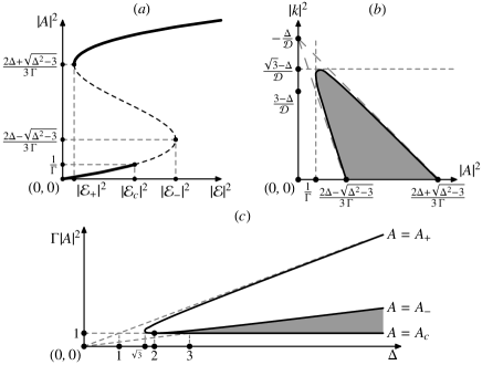
Figure 2: (a) Bistability curve of the intracavity intensity ($|{}{A}|^{2}$) vs driving intensity ($|\mathcal{E}|^{2}$). (b) Marginal stability curve. The domain of instability is filled. (c) Intracavity intensity vs detuning ($\Delta$). The plane is divided by the curves $A=A_{\pm}$ and $A=A_{\mathrm{c}}$, with $|{A_{\mathrm{c}}}|^{2}=1/\Gamma$ and $|{A_{\pm}}|^{2}=\left(2\Delta\pm\sqrt{\Delta^{2}-3}\right)/(3\Gamma)$. The domain of mi is filled.

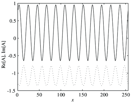
Figure 3: Stable dissipative structure emerging in the one-dimensional case when the resonator is biased near the threshold of mi. The real and imaginary parts of $A$ are plotted with solid and dotted lines, respectively. Parameters are $\Delta=10$, ${\delta}=-2$, $\Gamma=1$ and $\mathcal{E}=9.25$.

V Discussion

When the driving field amplitude is in the range $\mathcal{E}_{\mathrm{c}}<\mathcal{E}<\mathcal{E}_{-}$ and $\Delta>2$, a finite band of linearly unstable Fourier modes $k$ exist [see Fig. 2(b)], which trigger the spontaneous evolution of the intracavity field amplitude towards a stationary, spatially periodic distribution that occupies the whole cavity space available in the transverse directions. An example of a dissipative structure in the one-dimensional system obtained by numerical simulation of Eq. (8) is shown in Fig. 3. The initial condition consists of some small random noise added to the hss and periodic boundary conditions are assumed. To compare with the analytical results, we calculate the wavelength ($\Lambda_{\mathrm{c}}=3.14$) given by the linear stability analysis [Eq. (11)] and the wavelength of the stable dissipative structure obtained numerically ($\Lambda_{\mathrm{num}}=3.23$). A very good agreement between the two wavelengths is obtained. A weakly nonlinear analysis performed in the vicinity of the threshold for mi shows that the branch of periodic solutions always appears subcritically for $\Delta>\frac{41}{33}$. Changing the diffraction coefficient in these simulations will simply change the scaling of the pattern, as can be seen from Eq. (8) by nondimensionalizing $x$ and $y$ using the transformation $(x,y)=\sqrt{{\delta}}(X,Y)$. Since we can make the diffraction coefficient of the resonator under study as small as we desire by choosing the thicknesses of the two material layers appropriately, we can in principle produce dissipative structures with sizes smaller than the diffraction-limited size $\sqrt{l\mathcal{F}/(2\pi k_{0})}$. The combined use of lhms and rhms therefore enables us to circumvent the diffraction limit, which must be compared to the sub-diffraction-limited imaging of lhm plates Pendry (2000).

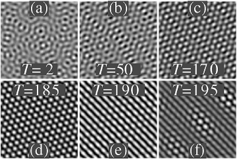
Figure 4: Dynamics of the pattern formation in the two-dimensional case. (a)–(b) Initial pattern formation. (c)–(d) Hexagonal structures emerge. (e) Hexagonal structures are replaced by stripes. (f) Self-organized spots appear. The labels correspond to the points (a)–(f) on Fig. 5. The parameters are the same as those in Fig. 3. Maxima are plain white and the integration mesh is $256\times 256$.

We carried out similar simulations in a square-shaped domain using periodic boundary conditions. The two-dimensional patterns are obtained by perturbing initially the hss in the same parameter range as in Fig. 3. The following sequence of transverse patterns is obtained: hexagons, stripes, and self-organized spots. This behavior is shown in Fig. 4(a)–(f), where we have plotted the real part of the intracavity field during the spatiotemporal evolution. From Fig. 5, we see that the average intensity grows exponentially, which is clearly due to the amplification of unstable wavelengths around $\Lambda_{\mathrm{c}}=2\pi/k_{c}$, as can be expected from the linear stability analysis. Finally, the field amplitude reaches the high hss. Note that the transition between the two hss is abrupt, but takes place after a fairly long transient close the lower hss branch. By varying the input field amplitude, we found that this phenomenon occurs for all input fields in the range $\mathcal{E}_{\mathrm{c}}<\mathcal{E}<\mathcal{E}_{-}$. This spontaneous spatiotemporal up-switching process therefore leads to the truncation of the homogeneous hysteresis cycle.

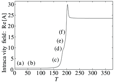
Figure 5: Time evolution during the two-dimensional up-switching process described. The average maximum value of the real part of the intracavity field is plotted.

To summarize, we presented a description of light propagation in a ring cavity filled with a left-handed and a right-handed material, both materials exhibiting a Kerr type nonlinearity. We derived a mean-field model for the spatiotemporal evolution of this resonator and showed that its diffraction coefficient can become negative if the thickness of the lhm layer is large enough. In this case, the lhm stabilizes the upper branch of the homogeneous steady state curve, and destabilizes a small part of the lower branch for high detuning ($\Delta>2$). In the latter parameter range, we demonstrated that pattern formation can take place. However, a spontaneous two-dimensional up-switching process dominates the spatiotemporal dynamics over the formation of stable patterns, resulting in the truncation of the homogeneous hysteresis cycle.

*

Appendix A Mean-field model

The mean-field approximation has already been applied to systems with boundary conditions Tlidi et al. (2000). Here, the propagation model is different, and we detail how it is possible to simplify the system of four coupled propagation equations, and the boundary conditions to only one equation of evolution, similar to the equation of the LL-model Lugiato and Lefever (1987).

A.1 Hypothesis and notations

We consider bidirectional propagation in a ring cavity with impedance matching at the interfaces between the two layers of classical and left-handed materials. In order to neglect the backward field with respect to the forward field in certain expressions, we also assume that the reflections at the other interfaces are limited. In cases where this assumption would not be verified, it is possible to add a circulator in the cavity, so that the condition holds.

Below, the letters $R$, $L$, and $C$ will refer to the field, nonlinearity and dispersion in, respectively , the right-handed medium, the left-handed medium, and the cavity outside of the two layers. The quantities $A$ and $B$ are (resp.) the envelope of the forward and the backward fields travelling in the ring cavity.

With theses notations, for example, $A_{C}(-l_{R})$ is the electric field outside the right-handed medium, in the entrance plane, while $A_{\mathrm{R}}(-l_{R})$ is the same field, at the same interface, but inside the medium.

The mean-field approximation consists in approximating the solution of the evolution in each layer, and for each forward or backward component as follows. In order to simplify the derivation, we rewrite Eq. (7) in the form

$$\frac{\partial A}{\partial\zeta}=i\left[{\mathcal{D}}+\mathcal{N}(A,B)\right]\,A,$$ (12)

where ${\mathcal{D}}$ is a linear differential operator, and $\mathcal{N}(A,B)$ a nonlinear operator, i.e.

$${\mathcal{D}} = \frac{1}{2k_{0}}\nabla^{2}_{\perp}-\frac{\beta_{2}}{2}\frac{\partial^{2}}{\partial{t}^{2}},$$ (13)

$$\mathcal{N} = \frac{3\omega_{0}}{2c\eta_{0}}\chi_{0}^{(3)}\left(\left|{A}\right|^{2}+\sigma\left|{B}\right|^{2}\right)A,$$ (14)

where $\sigma$ is the nonlinear coupling coefficient between the forward and the backward waves.

A.2 Boundary conditions

The geometry of the ring cavity leads to the following boundary conditions,

$$A_{C}(-l_{R}) = t_{in}\,E_{in}+r_{in}\,e^{i\,\varphi}\,A_{C}(l_{L}),$$ (15)

$$A_{R}(-l_{R}) = t_{R}\,A_{C}(-l_{R})+r_{R}\,B_{R}(-l_{R}),$$ (16)

$$A_{L}(0) = A_{R}(0),$$ (17)

$$A_{C}(l_{L}) = t_{L}\,A_{L}(l_{L})+r_{in}\,r_{L}\,e^{i\,\varphi}\,B_{C}(-l_{R}).$$ (18)

These expressions define the transmission and reflection coefficients at the interfaces. The phase factor $e^{i\,\varphi}$ accounts for the total phase accumulated in the ring cavity, outside of the two layers.

Similar relations can be written for the backward field,

$$B_{C}(-l_{R}) = t_{R}\,B_{R}(-l_{R})+r_{R}\,A_{C}(-l_{R}),$$ (19)

$$B_{L}(0) = B_{R}(0),$$ (20)

$$B_{L}(l_{L}) = t_{L}\,B_{C}(l_{L})+r_{L}\,A_{L}(l_{L}),$$ (21)

$$B_{C}(l_{L}) = r_{in}\,e^{i\,\varphi}\,B_{C}(-l_{R}).$$ (22)

A.3 Approximate equations of evolution

Assuming that $\delta\zeta=O(1)$, a first order integration of Eq. (12) leads to

$$A(\zeta+\delta\zeta) = A(\zeta)+i\delta\zeta\left[{\mathcal{D}}+\mathcal{N}(A,B)\right]|_{\zeta}\,A+O(2)$$

$$= e^{i\delta\zeta\left[{\mathcal{D}}+\mathcal{N}(A,B)\right]|_{\zeta}}\,A+O(2)$$

$$= e^{i\delta\zeta{\mathcal{D}}|_{\zeta}}e^{i\delta\zeta\mathcal{N}(A,B)|_{\zeta}}\,A+O(2)$$

$$= e^{i\delta\zeta\mathcal{N}(A,B)|_{\zeta}}e^{i\delta\zeta{\mathcal{D}}|_{\zeta}}\,A+O(2).$$

(23)

Now, we make the assumption that the reflection coefficients are small quantities ($r_{L}=O(1)=r_{R}$), and that the backward field is initially very weak ($B=O(1)$) in comparison with the forward field, so that

$$A_{C}(-l_{R}) = t_{in}\,E_{in}+r_{in}\,e^{i\,\varphi}\,A_{C}(l_{L}),$$ (24)

$$A_{R}(-l_{R}) = t_{R}\,A_{C}(-l_{R})+O(2),$$ (25)

$$A_{L}(0) = A_{R}(0),$$ (26)

$$A_{C}(l_{L}) = t_{L}\,A_{L}(l_{L})+O(2),$$ (27)

$$B_{C}(-l_{R}) = O(0)\,B_{R}(-l_{R})+O(1)\,A_{C}(-l_{R}),$$ (28)

$$B_{L}(0) = B_{R}(0),$$ (29)

$$B_{L}(l_{L}) = O(0)\,B_{C}(l_{L})+O(1)\,A_{L}(l_{L}),$$ (30)

$$B_{C}(l_{L}) = O(1)\,B_{C}(-l_{R}).$$ (31)

In addition, the first order integration of the propagation equation Eq. (23) shows that

$$A_{R}(0) = O(0)A_{R}(-l_{R}),$$ (32)

$$A_{L}(l_{L}) = O(0)A_{L}(0),$$ (33)

$$B_{R}(-l_{R}) = O(0)B_{R}(0),$$ (34)

$$B_{L}(0) = O(0)B_{L}(l_{L}).$$ (35)

From Eqs. (24)–(31), we deduce that

$$A = O(0)E_{in},$$ (37)

$$B = O(1)A.$$ (38)

This shows that the backward field will stay a first order quantity if it is initially so with respect to the forward field, and that we can neglect the linear coupling with the backward field in the boundary conditions Eqs. (24)–(27), or Eqs. (15)–(18), as the coupling is of second order.

The nonlinear coupling between the forward and the backward field is incoherent, meaning that it depends only on the intensity of the fields, and involves no exchange of energy between the two counterpropagating envelopes. This allows to relate, at first order, the forward and backward intensities everywhere in the cavity to the forward input intensity.

A reduction of Eqs. (15)–(18) and (23) provides

$$A^{(n)}(-l_{R})=$$

$$t_{in}\,E_{in}+r_{in}\,t_{L}\,t_{R}\,e^{i\,\varphi}\,\times$$

$$e^{i\,l_{L}\mathcal{N}_{L}}e^{i\,l_{L}{\mathcal{D}}_{L}}\,e^{i\,l_{R}{\mathcal{D}}_{R}}e^{i\,l_{R}\mathcal{N}_{R}}\,A^{(n-1)}(-l_{R}),$$

which expresses how the envelope of the forward field is related to both this same envelope one roundtrip before and the driving field $E_{in}$.

This discrete infinite set of equations can be reduced to a single equation, by introducing the roundtrip time $T$, and approximating the discrete variations by a partial derivative with respect to the slow time $\tau=n\,T$:

$$A^{(n)}-A^{(n-1)}\simeq T\left.\frac{\partial{A}}{\partial{\tau}}\right|_{\tau=n\,T}.$$ (41)

We find directly that

$$T\frac{\partial{A}}{\partial{\tau}}=t_{in}\,E_{in}+\left(\rho e^{i\,\mathcal{P}}-1\right)A,$$ (42)

where $\mathcal{P}=l_{L}{\mathcal{D}}_{L}+l_{R}{\mathcal{D}}_{R}+l_{L}\mathcal{N}_{L}+l_{R}\mathcal{N}_{R}$ accounts for the total propagation, and $\rho=r_{in}\,t_{L}\,t_{R}e^{i\,\varphi}$.

The backward field is proportional to the forward field, with $|{B_{C}(-l_{R})}|=|{r_{R}+r_{L}t_{L}t^{2}_{R}}||{A_{C}(-l_{R})}|+O(2)$, and similar expressions for $|{B_{R}(-l_{R})}|=\theta_{R}|{A_{R}(-l_{R})}|$, and $|{B_{L}(0)}|=\theta_{L}|{A_{R}(0)}|$. The exact expression of $\theta_{R}$ and $\theta_{L}$ is not important to complete our derivation. Below, it is only needed to remember that $\theta=O(1)$, and that $\theta$ is real.

The linear relation between the forward and the backward intensities simplifies the calculation of the nonlinear operators, as

$$\mathcal{N}(A,B)=\gamma\left(|{A}|^{2}+\sigma|{B}|^{2}\right)=\gamma\left(1+\sigma\theta^{2}\right)\,|{A}|^{2},$$ (43)

with $\gamma=\frac{3\omega_{0}}{2c\eta_{0}}\chi_{0}^{(3)}$.

By redefining $\gamma^{\prime}=\left(1+\sigma\theta^{2}\right)\gamma$, we can completely hide the existence of the backward field, that appears as a second order correction to the nonlinear coefficient. Therefore

$$\mathcal{P} = \frac{1}{2}\left(\frac{l_{L}}{k_{L}}+\frac{l_{R}}{k_{R}}\right)\nabla^{2}_{\perp}-\frac{1}{2}\left(l_{L}\beta_{2,L}+l_{R}\beta_{2,R}\right)\frac{\partial^{2}}{\partial{t}^{2}}$$ (44)

$$+ \left(l_{L}\gamma_{L}^{\prime}+l_{R}\gamma_{R}^{\prime}\right)\left|{A}\right|^{2}.$$

A.4 Lugiato-Lefever equation

Together, equations (42) and (44) fully describe the dynamics of the cavity. In this section, we will assume that we are working near resonance of the cavity, so as to obtain the standard form of the LL-model, after proper normalization of the coefficients.

Near resonance, $\rho=|\rho|e^{i\,\psi}$ is real, and $\psi$ accounts for the detuning with respect to the resonance ($\psi\approx 0$). In this particular case,

$$\rho e^{i\,\mathcal{P}}=|\rho|e^{i\,(\psi+\mathcal{P})}=|\rho|\left(1+i\psi+i\mathcal{P}\right)+O(2).$$ (45)

Introducing this expression in Eq. (42), we find

$$T\frac{\partial{A}}{\partial\tau}=t_{in}E_{in}+\left[\left(|\rho|-1\right)+i|\rho|\psi+i|\rho|\mathcal{P}\right]\,A.$$ (46)

This equation is similar to the LL-model, which appears more clearly, if we redefine

$$\tau^{\prime} = \frac{1-|\rho|}{T}\,\tau,$$ (47)

$$\mathcal{E}_{in} = \frac{t_{in}}{1-|\rho|}\,E_{in},$$ (48)

$$\Delta = -\frac{|\rho|}{1-|\rho|}\,\psi,$$ (49)

$$\delta = \frac{1}{2}\frac{|\rho|}{1-|\rho|}\left(\frac{l_{L}}{k_{L}}+\frac{l_{R}}{k_{R}}\right),$$ (50)

$$\beta = \frac{|\rho|}{1-|\rho|}\left(l_{L}\beta_{2,L}+l_{R}\beta_{2,R}\right),$$ (51)

$$\Gamma = \frac{|\rho|}{1-|\rho|}\left(l_{L}(1+\sigma\theta_{L}^{2})\gamma_{L}+l_{R}(1+\sigma\theta_{R}^{2})\gamma_{R}\right),$$

as in this case, the dynamics in the cavity near resonance is described by

$$\frac{\partial{A}}{\partial\tau^{\prime}}=\mathcal{E}_{in}-(1+i\Delta)A+i\delta\nabla^{2}_{\perp}A-i\frac{\beta}{2}\frac{\partial^{2}A}{\partial{t}^{2}}+i\Gamma|{A}|^{2}A.$$ (53)

When the system is driven by a continuous wave, the dispersive term disappears and we obtain Eq. (8). It is convenient to introduce the finesse of the cavity $\mathcal{F}=2\pi\frac{|\rho|}{1-|\rho|}$. If we neglect the second-order quantities $\theta$ and assume that $|\rho|\approx{}|{r_{in}}|=t_{in}=1/\sqrt{2}$, Eqs. (47)–(LABEL:eq:redim:f) lead to the simple form

$$\tau^{\prime} = \frac{\sqrt{2}\pi}{\mathcal{F}T}\,\tau,$$ (54)

$$\mathcal{E}_{in} = \frac{\mathcal{F}}{2\pi}\,E_{in},$$ (55)

$$\Delta = -\frac{\mathcal{F}}{2\pi}\,\psi,$$ (56)

$$\delta = \frac{\mathcal{F}}{4\pi}\left(\frac{l_{L}}{k_{L}}+\frac{l_{R}}{k_{R}}\right),$$ (57)

$$\Gamma = \frac{\mathcal{F}}{2\pi}\left(l_{L}\gamma_{L}+l_{R}\gamma_{R}\right).$$ (58)

References

- Glansdorff and Prigogine (1971) P. Glansdorff and I. Prigogine, Thermodynamic Theory of Structures, Stability and Fluctuations (Wiley, New York, 1971).
- Turing (1952) A. M. Turing, Phil. Trans. R. Soc. Lond. B 237, 37 (1952).
- Lange and Ackemann (2000) W. Lange and T. Ackemann, J. Opt. B : Quantum Semiclass. Opt. 2, 347 (2000).
- Rosanov (2002) N. N. Rosanov, Spatial Hysteresis and Optical Patterns (Springer, Berlin, 2002).
- Staliunas and Sanchez-Morcillo (2003) K. Staliunas and V. J. Sanchez-Morcillo, Transverse Patterns in Nonlinear Optical Resonators, Springer Tracts in Modern Physics (Springer-Verlag, Berlin Heidelberg, 2003).
- Mandel and Tlidi (2004) P. Mandel and M. Tlidi, J. Opt. B : Quantum Semiclass. Opt. 6, R60 (2004).
- Akhmediev and Ankiewicz (2005) N. Akhmediev and A. Ankiewicz, eds., Dissipative Solitons, vol. 661 of Lecture Notes in Physics (Springer, 2005).
- Moser et al. (2005) H. O. Moser, B. D. F. Casse, O. Wilhelmi, and B. T. Saw, Phys. Rev. Lett. 94, 063901 (2005).
- Grigorenko et al. (2005) A. N. Grigorenko, A. K. Geim, H. F. Gleeson, Y. Zhang, A. A. Firsov, I. Y. Khrushchev, and J. Petrovic, Nature 438, 335 (2005).
- Alù et al. (2006) A. Alù, A. Salandrino, and N. Engheta, Opt. Express 14, 1557 (2006).
- Linden et al. (2006) S. Linden, M. Decker, and M. Wegener, in Quantum Electronics and Laser Science Conference, QELS 2006 (The Optical Society of America (OSA), Long Beach, CA, USA, 2006), p. QThN4.
- Feth et al. (2006) N. Feth, C. Enkrich, D. Meisel, M. Wegener, C. Soukoulis, and S. Linden, in Quantum Electronics and Laser Science Conference, QELS 2006 (The Optical Society of America (OSA), Long Beach, CA, USA, 2006), p. QThN2.
- Zhang et al. (2006) S. Zhang, W. Fan, K. J. Malloy, S. R. J. Brueck, N. C. Panoiu, and R. M. Osgood, Jr., in Quantum Electronics and Laser Science Conference, QELS 2006 (The Optical Society of America (OSA), Long Beach, CA, USA, 2006), p. QWE6.
- Dolling et al. (2006) G. Dolling, C. Enkrich, M.Wegener, C. M. Soukoulis, and S. Linden, in Quantum Electronics and Laser Science Conference, QELS 2006 (The Optical Society of America (OSA), Long Beach, CA, USA, 2006), p. QWE3.
- Veselago (1968) V. G. Veselago, Sov. Phys. Usp. 10, 509 (1968).
- Shelby et al. (2001) R. A. Shelby, D. R. Smith, and S. Schultz, Science 292, 77 (2001).
- Wiltshire et al. (2001) M. C. K. Wiltshire, J. B. Pendry, I. R. Young, D. J. Larkman, D. J. Gilderdale, and J. V. Hajnal, Science 291, 849 (2001).
- Engheta (2002) N. Engheta, IEEE Antennas and Wireless Propagation Letters 1, 10 (2002).
- Feise et al. (2004a) M. W. Feise, I. V. Shadrivov, and Y. S. Kivshar, Appl. Phys. Lett. 85, 1451 (2004a).
- Hegde and Winful (2005) R. S. Hegde and H. G. Winful, Microwave and Optical Technology Letters 48, 528 (2005).
- Zharov et al. (2003) A. A. Zharov, I. V. Shadrivov, and Y. S. Kivshar, Phys. Rev. Lett. 91, 37401 (2003).
- Agranovich et al. (2004) V. M. Agranovich, Y. R. Shen, R. H. Baughman, and A. A. Zakhidov, Phys. Rev. B 69, 165112 (2004).
- Feise et al. (2004b) M. W. Feise, I. V. Shadrivov, and Y. S. Kivshar, Appl. Phys. Lett. 69, 1451 (2004b).
- Lazarides and Tsironis (2005) N. Lazarides and G. P. Tsironis, Phys. Rev. E 71, 049903 (2005).
- Zharov et al. (2005) A. A. Zharov, N. A. Zharova, I. V. Shadrivov, and Y. S. Kivshar, Appl. Phys. Lett. 87, 091104 (2005).
- Shadrivov et al. (2006) I. V. Shadrivov, A. A. Zharov, and Y. S. Kivshar, J. Opt. Soc. Am. B 23, 529 (2006).
- Gabitov et al. (2006) I. R. Gabitov, N. M. Lichtinitser, and A. I. Maimitsov, in Conference on Lasers and Electro-Optics, CLEO 2006 (The Optical Society of America (OSA), Long Beach, CA, USA, 2006), p. JThC18.
- Conti and Trillo (1988) C. Conti and S. Trillo, Opt. Lett. 13, 794 (1988).
- Christodoulides and Joseph (1988) D. N. Christodoulides and R. I. Joseph, Opt. Lett. 13, 794 (1988).
- Eisenberg et al. (2000) H. S. Eisenberg, Y. Silberberg, R. Morandotti, and J. S. Aitchison, Phys. Rev. Lett. 85, 1863 (2000).
- Staliunas (2003) K. Staliunas, Phys. Rev. Lett. 91, 053901 (2003).
- Lapine et al. (2003) M. Lapine, M. Gorkunov, and K. H. Ringhofer, Phys. Rev. E 67, 065601 (2003).
- Moloney and Newell (2003) J. V. Moloney and A. C. Newell, Nonlinear Optics (Westview Press, Boulder, Colorado, 2003).
- Tassin et al. (2005) P. Tassin, G. Van der Sande, I. Veretennicoff, M. Tlidi, and P. Kockaert, Proc. SPIE 5955, 59550X (2005).
- Lugiato and Lefever (1987) L. A. Lugiato and R. Lefever, Phys. Rev. Lett. 58, 2209 (1987).
- Pendry (2000) J. B. Pendry, Phys. Rev. Lett. 85, 3966 (2000).
- Tlidi et al. (2000) M. Tlidi, M. Le Berre, E. Ressayre, A. Tallet, and L. Di Menza, Phys. Rev. A 61, 043896 (2000).