Surface-wave solitons on the interface between a linear medium and a nonlocal nonlinear medium

Abstract

We address the properties of surface-wave solitons on the interface between a semi-infinite homogeneous linear medium and a semi-infinite homogeneous nonlinear nonlocal medium. The stability, energy flow and FWHM of the surface wave solitons can be affected by the degree of nonlocality of the nonlinear medium. We find that the refractive index difference affects the power distribution of the surface solitons in two media. We show that the different boundary values at the interface can lead to the different peak position of the surface solitons, but it can not influence the solitons stability with a certain degree of nonlocality.

Surface waves propagating along the interface between a homogeneous linear medium and a homogeneous nonlinear medium display many interesting properties, which have no analogues in homogeneous media. Decades years ago, such surface waves had been studied in the local nonlinear optical case ref1 ; ref2 ; ref3 ; ref4 ; ref5 ; ref6 . [1] and [6] show that there is no stable surface wave when the zero field refractive index of the nonlinear medium is larger than the refractive index of the linear medium, on the contrary, surface wave is stable.

In the nonlocal nonlinear optical domain, such surface waves were analyzed at the interfaces of diffusive Kerr-type materials ref7 ; ref8 ; ref9 . Recently, surface-wave solitons were observed at the interface between a dielectric medium(air) and a nonlocal nonlinear medium(lead glasses) ref10 . They found that these solitons are always attracted toward the surface, and unlike their Kerr-like counterparts, they do not exhibit a power threshold. Two-dimensional surface solitons featuring topologically complex shapes, including vortices and dipoles with nodal lines perpendicular to the interface of nonlocal thermal media were studied in [11]. Defocusing thermal materials can also support surface waves under appropriate conditions ref12 ; ref13 . Multiploe solitons localized at a thermally insulating interface are addressed in [14].

However, to our knowledge, the variation of such surface-wave solitons due to the change of the degree of nonlocality or the boundary value at the interface of the semi-infinite nonlocal nonlinear media and the semi-infinite linear media were not studied to this day. In this Letter, we reveal that the degree of nonlocality can affect the stability, the energy flow and the full width at half maximum(FWHM) of the surface solitons. We state that the refractive index difference affects the power distribution of the surface solitons in two media. In addition, we show that the different boundary values at the interface can lead to the different peak position of the surface solitons, but it can not influence the solitons stability with a certain degree of nonlocality.

Here, we consider the simple (1+1)D case. $x=0$ is the interface of the nonlinear medium(a linear refractive index $n_{L}$) and a linear medium of refractive index $n_{0}$. To describe the propagation of light beams along $Z$ axis near the interface of the nonlinear medium, we use a nonlinear Schröinger equation for the dimensionless amplitude $a$ of the light field coupled to the equation for normalized nonlinear induced change of the refractive index $\phi$,

$$i\partial_{Z}a+\frac{1}{2}\frac{\partial^{2}a}{\partial X^{2}}+\frac{w_{0}^{2}}{2}(k_{0}^{2}n_{L}^{2}-\beta^{2})a+\phi a=0,\textrm{for}-\infty\leq X\leq 0,$$ (1a)

$$i\partial_{Z}a+\frac{1}{2}\frac{\partial^{2}a}{\partial X^{2}}+\frac{w_{0}^{2}}{2}(k_{0}^{2}n_{0}^{2}-\beta^{2})a=0\quad\textrm{for}\quad 0\leq X\leq\infty.$$ (1b)

and

$$\alpha^{2}\nabla_{\bot}^{2}\phi-\phi+|a|^{2}=0\quad\textrm{for}-\infty\leq X\leq 0.$$ (2)

where $X$ is is the transverse coordinate, $\alpha^{2}=w_{m}^{2}/w_{0}^{2}$, $w_{0}$ is the beam width, $w_{m}$ is the characteristic length of the nonlinear response and $\alpha$ stands for the degree of nonlocality of the nonlinear response. $\beta$ and $k_{0}=2\pi/\lambda$ are the wave numbers in the media and in vacuum. $\phi$ is given by $\phi(X)=\phi_{0}e^{X/\alpha}-(1/\alpha^{2})\int^{0}_{-\infty}G(X,\xi)|a(\xi)|^{2}d\xi$, where $G(X)=\alpha e^{\xi/\alpha}(e^{X/\alpha}-e^{-X/\alpha})/2$, for $X\geq\xi$, and $G(X)=\alpha e^{X/\alpha}(e^{\xi/\alpha}-e^{-\xi/\alpha})/2$, for $X\leq\xi$. Here, we can safely assume that the boundary condition at the interface($X=0$) is $\phi=\phi_{0}(\phi_{0}>0)$, where $\phi_{0}=50$ is the initial value, unless we indicate it. $a$ and $\phi$ vanish at the $X\rightarrow\pm\infty$.

We search for stationary soliton solutions of Eqs. (1) and (2) numerically in the form $a(X,Y,Z)=u(X,Y)\exp(ibZ)$, where $u$ is the real function and $b$ is a real propagation constant of spatial solitons in the normalized system.

$$\frac{1}{2}\nabla_{\bot}^{2}u-bu+\frac{w_{0}^{2}}{2}(k_{0}^{2}n_{L}^{2}-\beta^{2})u+\phi u=0,$$ (3a)

$$\frac{1}{2}\nabla_{\bot}^{2}u-bu+\frac{w_{0}^{2}}{2}(k_{0}^{2}n_{0}^{2}-\beta^{2})u=0.$$ (3b)

and

$$\alpha^{2}\nabla_{\bot}^{2}\phi-\phi+|u|^{2}=0.$$ (4)

To elucidate the linear stability of the solitons, we searched for perturbed solutions in the form $a(X,Z)=[u(X)+p(X,Z)+iq(X,Z)]\exp(ibZ)$ ref9 ; ref12 ; ref14 ; ref15 , where the real $p(X,Z)$ and imaginary $q(X,Z)$ parts of the perturbation can grow with a complex rate $\delta=\delta_{r}+i\delta_{i}$ upon propagation. Linearization of Eq.(3)and (4) around a stationary solution yields the eigenvalue problem

$$\delta p=-\frac{1}{2}\frac{\partial^{2}q}{\partial X^{2}}+bq-\phi q-\frac{w_{0}^{2}}{2}(k_{0}^{2}n_{L}^{2}-\beta^{2})q,$$ (5a)

$$\delta q=\frac{1}{2}\frac{\partial^{2}p}{\partial X^{2}}-bp+\phi p+\frac{w_{0}^{2}}{2}(k_{0}^{2}n_{L}^{2}-\beta^{2})p-u\Delta\phi.$$ (5b)

which holds for $-\infty\leq X\leq 0$. where $\Delta\phi=2\int^{0}_{-\infty}G(X,\xi)u(\xi)p(\xi)d\xi$.

For $0\leq X\leq\infty$, the eigenvalue problem

$$\delta p=-\frac{1}{2}\frac{\partial^{2}q}{\partial X^{2}}+bq-\frac{w_{0}^{2}}{2}(k_{0}^{2}n_{0}^{2}-\beta^{2})q,$$ (6a)

$$\delta q=\frac{1}{2}\frac{\partial^{2}p}{\partial X^{2}}-bp+\frac{w_{0}^{2}}{2}(k_{0}^{2}n_{0}^{2}-\beta^{2})q.$$ (6b)

We first consider that the influence of the difference of $n_{L}$ and $n_{0}$ on the surface solitons. For the zero field refractive index of the nonlinear medium($n_{L}$) is larger than the refractive index of the linear medium($n_{0}$), at the same degree of nonlocality of the nonlinear response, from Fig. 1, we can find that the solitons reside almost fully inside the nonlocal nolinear region and only weakly penetrate into the linear region when two media have a large refractive index difference, but the surface solitons have a significant part of their optical power residing in the linear medium when the boundary is between two media with a small refractive index difference which is comparable to the nonlinear index change. The results show that the refractive index difference affects the power distribution of the surface solitons in two media. Comparing Fig. 1(b) with (c), we can see that the profiles of surface solitons are alike when the refractive index difference between two media is small. However, when the refractive index difference between two media is big(Fig. 1(a) and (d)), the profiles of solitons are very different and solitons are no longer affected by nonlocality shown in Fig. 2(d)($n_{0}-n_{L}=0.6$). Of course, when the degree of nonlocality $\alpha$ is equal to zero, that is to say, the nonlinear media is local, the solitons are stable in the case of Fig. 1(c), whereas the solitons are unstable in the case of Fig. 1(b) ref1 ; ref6 .

The central finding in this Letter is the influence of the change of nonlocal degree on the solitons stability. In Fig. 2(a), for $n_{L}>n_{0}$, with the degree of nonlocality becomes stronger, the solitons are more stable. When the degree of nonlocality exceeds a certain value, the solitons will be stable. The index difference influences the value. For $n_{L}<n_{0}$, only when the index difference is small, the solitons stability will be affected by the degree of nonlocality. This is shown in Fig. 2(c). Fig. 2(b) and (d) depict the solitons are very stable, propagating without distortion or deviations in their trajectories for a propagation distance of $15$ diffraction lengths with 5% white noise. These results illustrate the fact that the nonlocal nonlinearity does action on the surface soltions. when the force exerted on the beam by the nonlocal nonlinearity is equal to the force exerted by the boundary at the interface, the solitons keep their straight line trajectories. Here, we only show that the cases $n_{L}-n_{0}=0.6$[Fig. 2(b)] and $n_{0}-n_{L}=1\times 10^{-6}$[Fig. 2(d)]. Having demonstrated the influence of the degree of nonlocality on stability of the surface solitons, we proceed to study the energy flow $P=\int^{\infty}_{-\infty}|a|^{2}dX$ or FWHM of the surface solitons as a function of the degree of nonlocality $\alpha$[Fig. 3]. As the degree of nonlocality increase, the energy flow monotonously increases. FWHM firstly increases with the increase of $\alpha$, but it will decrease when the degree of nonlocality is strongly nonlocal. Importantly, the boundary value at the interface can also dramatically modify the properties of surface soltions. For example, it can affect the position $X_{max}$ of the maximum value of $|u|$ [Fig. 4(a)]. $X_{max}$ is located farther away from the interface when the boundary value $\phi_{0}$ is smaller. In Fig. 4(b) and (c), one can easily find this point by comparing the surface soltion at $\phi_{0}=20$ with the surface soltion at $\phi_{0}=50$. So, we can say that the force exerted on the surface solitons by the interface will increase when the boundary value increases. The force attracts the surface solitons to the interface. However, the boundary value at the interface can not influence the stability of solitons when $\alpha$ is a certain value. This can be explained by Fig. 4(d) in which the change of the perturbation growth rate $\delta_{r}$ followed by $\phi_{0}$ is a straight line.

To summary, the stability, energy flow and FWHM of the surface wave solitons can be affected by the degree of nonlocality of the nonlinear medium. We find that the refractive index difference affects the power distribution of the surface solitons in two media. We state that the different boundary values at the interface can lead to the different peak position of the surface solitons, but it can not influence the solitons stability with a certain degree of nonlocality.

This research was supported by the Specialized Research Fund for the Doctoral Program of Higher Education (Grant No. 20060574006), and Program for Innovative Research Team of the Higher Education in Guangdong (Grant No. 06CXTD005).

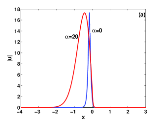
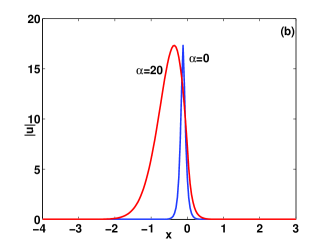
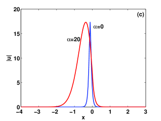
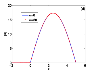
Figure 1: Profiles of surface solitons at $\alpha=0$, and $\alpha=20$ for (a)$n_{L}-n_{0}=0.6$ , (b)$n_{L}-n_{0}=1\times 10^{-6}$, (c)$n_{0}-n_{L}=1\times 10^{-6}$ and (d) $n_{0}-n_{L}=0.6$.

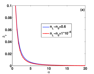
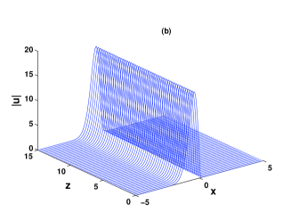
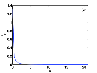
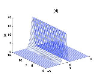
Figure 2: The influence of the degree of nonlocality $\alpha$ on the perturbation growth rate $\delta_{r}$ for $n_{L}-n_{0}=0.6$ or $n_{L}-n_{0}=1\times 10^{-6}$(a) and $n_{0}-n_{L}=1\times 10^{-6}$(c). Propagation of the surface solitons launched at $x=0$ with 5% noise at $\alpha=20$ for $n_{L}-n_{0}=0.6$(b) and $n_{0}-n_{L}=1\times 10^{-6}$(d).

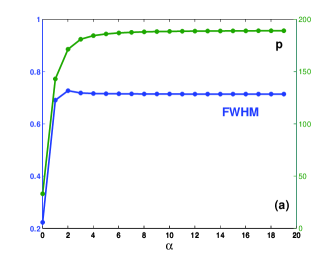
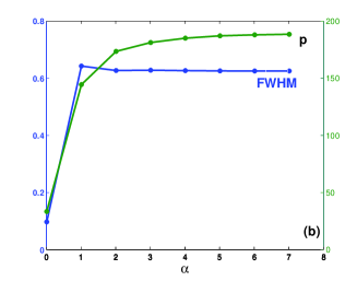
Figure 3: Energy flow $P$ and FWHM versus $\alpha$ for surface solitons for $n_{L}-n_{0}=0.6$(a) and $n_{0}-n_{L}=1\times 10^{-6}$(b).

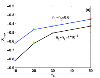
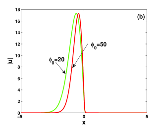
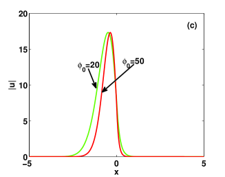
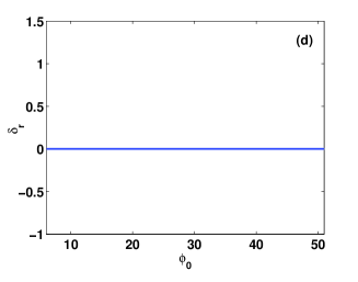
Figure 4: (a)The position $X_{max}$ of the maximum value of $|u|$ as a function of the boundary value $\phi_{0}$ at the surface. Circles correspond to surface soltion at $\phi_{0}=20$ or $\phi_{0}=50$ shown in (b) for $n_{L}-n_{0}=0.6$ and (c) for $n_{0}-n_{L}=1\times 10^{-6}$. (d) The influence of $\phi_{0}$ on $\delta_{r}$. $\alpha=20$ for all figures.

References

- (1) W. J. Tomlinson, Opt. Lett. 5, 323-325 (1980).
- (2) N. N. Akhmediev, V. I. Korneev, and Y. V. Kuz menko, Sov. Phys. JETP 61, 62-67 (1985).
- (3) K. M. Leung, Phys. Rev. B. 32, 5093-5101 (1985).
- (4) A. D. Boardman. A. A. Maradudin, G. I. Stegeman, T. Twardowski and E. M. Wright, Phys. Rev. A. 35, 1159-1164 (1987).
- (5) D. Mihalache, G. Stegeman, C. T. Seaton, R. Zanoni, A. D. Boardman and T. Twardowski, Opt. Lett. 12, 187-189 (1987).
- (6) Shigeaki Ohke, Tokuo Umeda and Yoshio Cho, Electron. Comm. Jpn. 2. 75, 57-66 (1992).
- (7) P. Varatharajah, A. Aceves, J. V. Moloney, D. R. Heatley, and E. M. Wright, Opt. Lett. 13, 690-692 (1988).
- (8) D. R. Andersen, Phys. Rev. A 37, 189-193 (1988).
- (9) Y. V. Kartashov, L. Torner, and V. A. Vysloukh, Opt. Lett. 31, 2595-2597 (2006).
- (10) B. Alfassi, C. Rotschild, O. Manela, M. Segev, and D. N. Christodoulides, Phys. Rev. Lett. 98, 213901 (2007).
- (11) F. Ye, Y. V. Kartashov, and L. Torner, ”Nonlocal surface dipoles and vortices,” Phys. Rev. A 77, 033829 (2008).
- (12) Y. V. Kartashov, F. Ye, V. A. Vysloukh, and L. Torner, Opt. Lett. 32, 2260-2262 (2007).
- (13) Y. V. Kartashov, V. A. Vysloukh, and L. Torner, Opt. Express 15, 16216-16221 (2007).
- (14) Y. V. Kartashov, V. A. Vysloukh, and L. Torner, Opt. Lett. 34, 283-285 (2009).
- (15) Z. Xu, Y. V. Kartashov, V. A. Vysloukh, and L. Torner, Opt. Lett. 30, 3171-3173 (2005).