Cosmic Behavior, Statefinder Diagnostic and $w-w^{\prime}$ Analysis for
Interacting NADE model in Non-flat Universe

Abstract

We give a brief review of interacting NADE model in non-flat universe. we study the effect of spatial curvature $\Omega_{k}$, interaction coefficient $\alpha$ and the main parameter of NADE, $n$, On EoS parameter $w_{d}$ and deceleration parameter $q$. We obtain a minimum value for $n$ in both early and present time, in order to that our DE model crosses the phantom divide. Also in a closed universe, changing the sign of $q$ is strongly dependent on $\alpha$. It has been shown that the quantities $w_{d}$ and $q$ have a different treatment for various spatial curvature. At last, we calculate the statefinder diagnostic and $w-w^{\prime}$ analysis in non flat universe. In non flat universe, the statefinder trajectory is discriminated by both $n$ and $\alpha$.

I Introduction

The observational data of Ia supernova(SNIa) SN , large scale structure (LSS) LSS and cosmic microwave background (CMB) anisotropy CMB show that the universe is undergoing an accelerating expansion. It is believed that a dark energy with negative pressure can drive this accelerated expansion. The dark energy (DE) problem attracted a great deal of attention in the last decade. Up to now, many models such as $\Lambda$CDM , the models with a scalar field and modified gravity had been proposed Pad .Also in the last decade the other models base on quantum field theory such as holographic hol and agegraphic (ADE) Cai1 dark energy models are suggested. The latter is arisen from combining quantum mechanics with general relativity directly. It is worthwhile to mention that up to now, a completely successful quantum theory of gravity is not available. There are two main problems in dealing with $\Lambda$CDM model which are ’fine-tuning’ and ’cosmic coincidence’ problem copel . The ADE model, which is proposed by Cai Cai1 , is based on the line of quantum fluctuations of spacetime, the so-called Károlyházy relation $\delta t=\lambda t_{p}^{2/3}t^{1/3}$, and the energy-time Heisenberg uncertainty relation $E_{\delta t^{3}}\sim t^{-1}$. These relations enable one to obtain an energy density of the metric quantum fluctuations of Minkowski spacetime as follows Maz

$$\rho_{q}\sim\frac{E_{\delta t^{3}}}{\delta t^{3}}\sim\frac{1}{t_{p}^{2}t^{2}}\sim\frac{m_{p}^{2}}{t^{2}}.$$ (1)

Throughout this paper, we use the Plank unit ($\hbar=c=k_{B}=1$) , where $t_{p}=l_{p}=1/m_{p}$ are Plank’s time, length and mass, respectively. In ADE, this energy density is considered as density of dark energy component, $\rho_{d}$, of spacetime. By considering a Friedmann-Robertson-Walker (FRW) universe, due to effect of curvature, one should introduce a numerical factor $3n^{2}$ in (1) cai2 ; cai3 .

By making a model that considering DE, independent of the other mater fields, one can study the evolution of characteristics of dark energy of spacetime very well. The recent observational data from the Abell Cluster $A586$ supports the interaction between dark matter and dark energy bertol . However, the strength of this interaction is not exactly identified feng . Also, nowadays, many authors are interested to consider non-flat FRW universe shikh ; karami . The tendency of a closed universe is shown in a suite CMB experiments Sie . Besides of it, the measurements of the cubic correction to the luminosity-distance of supernova measurements reveal a closed universe Caldwell . In accordance of all mentioned above, we prefer to consider a model including dark matter and dark energy for a non-flat FRW universe.

The interacting new ADE (NADE) which is a new version of ADE with a conformal time instead of a cosmic time in FRW metric. The motivation of this new model is for that the original ADE model cannot explain the matter-dominated era cai4 . Recently, the interacting NADE model has been investigated and some cosmological quantities such as deceleration parameter $q$, evolution behavior of fractional dark energy density $\Omega_{d}^{\prime}$, and equation of state (EOS) parameter $w_{d}=P_{d}/\rho_{d}$, are obtained wei ; zhang .

The next step beyond Hubble parameter $H=\dot{a}/a$ and $q=-\ddot{a}/aH^{2}$, is to consider a new quantity contains $\dddot{a}$. A pair quantities which have been introduced by Sahni et al. and Alam et al. Sahni , are called statefinder pair {r,s}, as

$$r=\frac{\dddot{a}}{aH^{3}},~{}~{}~{}~{}~{}~{}~{}s=\frac{r-1}{3(q-1/2)},$$ (2)

The statefinder pair is a geometrical diagnostic tool which is constructed directly from a spacetime metric. The importance of such pair is to distinguish of the cosmological evolution behaviors of dark energy models with the same values of $H_{0}$ and $q_{0}$ at the present time. At future by combining the data of Supernova acceleration probe (SNAP) with statefinder diagnosis, we may choose the best model of dark energy. Up to now, many authors have investigated statefinder trajectories for standard $\Lambda$CDM model and quintessence r9 ; r10 , interacting quintessence models r12 ; r13 , chaplygin gas, the holographic dark energy models r14 ; r15 , the holographic dark energy model in non-flat universe r16 , the phantom model r18 , the tachyon r22 , the ADE model with and without interaction wei and the interacting NADE model in flat universe zhang . They had shown the statefinder diagnosis is a useful tool for discrimination between various dark energy models. In addition to the statefinder geometrical diagnostic, the another tool to distinguish between the different models of dark energy is $w-w^{\prime}$ analysis which is used extensively in the literature wei ; wwp .

In this paper, in addition of cosmic behavior investigation, we study the statefinder trajectories and $w-w^{\prime}$ analysis for interacting NADE model in a non-flat FRW universe.

II COSMIC EVOLUTION IN NON-FLAT UNIVERSE WITH INTERACTING NADE

As we mentioned in Sec. (I), the energy density can be defined in ADE model as

$$\rho_{d}=\frac{3n^{2}m_{p}^{2}}{T^{2}}$$ (3)

where the cosmic time $T$ is defined as the age of the universe

$$T=\int dt=\int_{0}^{a}\frac{da}{Ha}.$$ (4)

Introducing a conformal time $\eta$ which is defined as $dt=ad\eta$, the FRW universe is modified as

$$ds^{2}=dt^{2}-a^{2}dx^{2}=a^{2}(d\eta^{2}-dx^{2}).$$ (5)

Therefore, by substituting the time scale $\eta$ in Eq.(3), one can obtain the energy density of NADE model as

$$\rho_{d}=\frac{3n^{2}m_{p}^{2}}{\eta^{2}};\qquad\eta=\int\frac{dt}{a}=\int_{0}^{a}\frac{da}{Ha^{2}};\qquad\dot{\eta}=\frac{1}{a}.$$ (6)

The corresponding fractional energy density is

$$\Omega_{d}=\frac{n^{2}}{H^{2}\eta^{2}}.$$ (7)

The Friedmann equation of a non-flat FRW universe containing a new agegraphic dark energy and pressureless matter (baryons and dark matter) is

$$H^{2}+\frac{k}{a^{2}}=\frac{1}{3m_{p}^{2}}(\rho_{m}+\rho_{d})$$ (8)

where $k=1,0,-1$ is curvature parameter corresponding to closed, flat and open universe, respectively. Some recent observations reveal a closed universe with a present small fractional energy density $\Omega_{k0}=1/H_{0}^{2}\simeq 0.02$ Bennet . Also we can write the Friedmann equation (8) in to another form with respect to fractional energy density $\Omega_{i}=\rho_{i}/\rho_{c}$, with $\rho_{c}=3m_{p}^{2}H^{2}$. Then we have

$$\Omega_{m}+\Omega_{d}=1+\Omega_{k}.$$ (9)

The continuity equations including an interaction term between dark matter and dark energy become

$$\dot{\rho_{m}}+3H\rho_{m} = Q,$$ (10)

$$\dot{\rho_{d}}+3H(\rho_{d}+p_{d}) = -Q,$$ (11)

where $p_{d}$ is dark energy pressure which is given by equation of state (EoS), $w_{d}=p_{d}/\rho_{d}$. Three forms of $Q$ which have been extensively used in literatures cai4 ; zhang ; shikh are

$$Q=9\alpha_{i}m_{p}^{2}H^{3}\Omega_{i};\qquad\Omega_{i}=\left\{\begin{array}[]{ll}\Omega_{d};&i=1\\ \vspace{0.75mm}\Omega_{m};&i=2\\ \Omega_{d}+\Omega_{m};&i=3\end{array}\right..$$ (12)

Differentiating Eq. (7) and using Eqs. (3), (8) and (9), the derivative of $\Omega_{d}$ can be calculated as

$$\Omega_{d}^{\prime} = \frac{\dot{\Omega}}{H}=-2\Omega_{d}\left[\frac{\dot{H}}{H^{2}}+\frac{\sqrt{\Omega_{d}}}{na}\right];$$ (13)

$$\frac{\dot{H}}{H^{2}} = -\frac{\Omega_{d}^{3/2}}{na}-\frac{3}{2}(1-\Omega_{d})-\frac{\Omega_{k}}{2}+\frac{Q_{c}}{2},$$ (14)

where prime denotes the derivative with respect to $\ln a$ and $Q_{c}=Q/H\rho_{c}=3\alpha_{i}\Omega_{i}.$ The relations (13) and (14), also has been obtained in shikh for third interaction form of $Q.$

Using the relation (14) in (13), we obtain a normal differential equation for $\Omega_{d}$ as

$$\Omega_{d}^{\prime}=\Omega_{d}\left[(1-\Omega_{d})(3-2\frac{\sqrt{\Omega_{d}}}{na})+\Omega_{k}-Q_{c}\right],$$ (15)

where $\Omega_{k}$ is given by

$$\Omega_{k}=\frac{a\gamma(1-\Omega_{d})}{1-a\gamma}.$$ (16)

Hear $\gamma$ is satisfied in the following equation

$$\frac{\Omega_{k}}{\Omega_{m}}=a\frac{\Omega_{k0}}{\Omega_{m0}}=a\gamma.$$ (17)

From Eqs. (6), (7) and (11), the EoS parameter can be obtained as

$$w_{d}=-1-Q_{cd}+\frac{2\sqrt{\Omega_{d}}}{3na},$$ (18)

where $Q_{cd}=Q_{c}/(3\Omega_{d})$. The evolution behavior of $w_{d}$ (18) by using (15), is given by

$$w_{d}^{\prime}=+\frac{\sqrt{\Omega_{d}}}{3na}\left[1+\Omega_{k}-3\Omega_{d}-2\frac{\sqrt{\Omega_{d}}}{na}(1-\Omega_{d})-Q_{c}\right]-Q_{cd}^{\prime}.$$ (19)

Also the total EoS parameter is obtained as

$$w_{tot}=\frac{p_{tot}}{\rho_{tot}}=\frac{\Omega_{d}w_{d}}{1+\Omega_{k}}.$$ (20)

To achieve an accelerated expansion, it is required that $w_{tot}$ $<-1/3$. Therefore at present time in a closed universe ($a=1,\Omega_{k0}=0.02,$ $\Omega_{d0}=0.72$), the minimum value of $n$ with $\alpha_{i}=0.1$ for various forms of $Q,$ can be obtained as

$$n\geq\left\{\begin{array}[]{ll}0.901;&i=1\\ \vspace{0.75mm}0.993;&i=2\\ 0.845;&i=3\end{array}\right.$$ (21)

In interacting NADE, based on Eq. (18) , we see that at present time, $w_{d}$ can cross the phantom divide ($w<-1$) provided

$$n\alpha\geq\left\{\begin{array}[]{ll}0.566;&i=1\\ 1.358;&i=2\\ 0.399;&i=3\end{array}\right.$$ (22)

The third value of (22), has been also expressed in shikh . The relation (22) show that for the same value of $\alpha$, $n_{i}$ is increasing by moving from $i=3$ in to $i=1$ and then $i=2.$

The deceleration parameter $q$ can be calculated from Eqs. (13) and (15) as

$$q = -\frac{\dot{H}}{H^{2}}-1=\frac{(1+\Omega_{k})}{2}+\frac{3}{2}\Omega_{d}w_{d}$$ (23)

$$= \frac{\Omega_{d}^{3/2}}{na}-\Omega_{d}+\frac{1-\Omega_{d}}{2(1-a\gamma)}-\frac{Q_{c}}{2}$$ (24)

III STATEFINDER DIAGNOSTIC OF NADE IN INTERACTING NON-FLAT UNIVERSE

Now we find the statefinder pair {r,s}, which was expressed in Sec.I. From the definition of $q$ and $H$, the parameter $r$ (2) can be written as

$$r=\frac{\ddot{H}}{H^{3}}-3q-2.$$ (25)

Using Eqs. (14), (18) and (23) we have

$$\frac{\ddot{H}}{H^{3}}=\frac{9}{2}+\frac{9}{2}\Omega_{d}w_{d}(w_{d}+Q_{cd}+2)-\frac{3}{2}\Omega_{d}w_{d}^{\prime}+\frac{5}{2}\Omega_{k}.$$ (26)

Hence, the Eq. (25) can be obtained as

$$r=1+\Omega_{k}+\frac{9}{2}\Omega_{d}w_{d}(w_{d}+Q_{cd}+1)-\frac{3}{2}\Omega_{d}w_{d}^{\prime}.$$ (27)

In a non flat universe, Evans et al. Evans generalize the definition of parameter $s$ (2) as

$$s=\frac{r-\Omega_{tot}}{\frac{3}{2}(q-\frac{\Omega_{tot}}{2})},$$ (28)

where the total fractional energy density is $\Omega_{tot}=\Omega_{m}+\Omega_{d}=1+\Omega_{k}$. Therefore from this new definition we have

$$s=1+w_{d}+Q_{cd}-\frac{w_{d}^{\prime}}{3w_{d}}.$$ (29)

The relations (26),(27) and (29) reduced to (35), (37) and (38) of Ref. zhang in the limiting case of flat universe. By omitting $w_{d}^{\prime}$ between (27) and (29), we find $r$ in terms of $s$ as follows

$$r=1+\Omega_{k}+\frac{9}{2}s\Omega_{d}w_{d}.$$ (30)

IV Numerical results

In this section, first we give the complete numerical description of the NADE model and then examine the NADE model with statefinder diagnostic tool and $w-w^{\prime}$ analysis. Here we consider the first case of interaction form, $Q=Q_{1}=9\alpha_{1}m^{2}H^{3}\Omega_{d}$, in (12) with $\alpha=\alpha_{1}$. In this case, the differential equation for $\Omega_{d}$ (15) can be reduced as

$$\Omega_{d}^{\prime}=\Omega_{d}[(1-\Omega_{d})(3-\frac{2\sqrt{\Omega_{d}}}{na})-3\Omega_{d}\alpha+\Omega_{k}]$$ (31)

Substituting $Q_{1}$ in Eqs.(18), (19), (27) and (29), yields the following equations:

$$w_{d}=-1+\frac{2\sqrt{\Omega_{d}}}{3na}-\alpha$$ (32)

$$w_{d}^{\prime}=\frac{\sqrt{\Omega_{d}}}{3na}[(1+\Omega_{k})-3\Omega_{d}(1+\alpha)-\frac{2\sqrt{\Omega_{d}}}{na}(1-\Omega_{d})]$$ (33)

$$r=1+\Omega_{k}+\frac{9}{2}\Omega_{d}w_{d}(w_{d}+\alpha+1)-\frac{3}{2}\Omega_{d}w_{d}^{\prime}.$$ (34)

$$s=1+w_{d}+\alpha-\frac{w_{d}^{\prime}}{3w_{d}}.$$ (35)

Because of vanishing $\Omega_{d}$ at $a\rightarrow 0$, the second term of Eq.(32) can be larger or smaller than unity at this time. This term is examined by numerical analysis and we see that it is much lower than one for higher values of model parameter $n$. Hence, NADE model can cross the phantom divide ($w_{d}<-1$) at $a\rightarrow 0$, independent of the contribution of the spatial curvature of the universe.

On the other hand, at the late time (e.g., $a\rightarrow\infty$) when $\Omega_{d}\rightarrow 1$, $w_{d}$ tends to $-1$ and NADE model mimics the cosmological constant. Here we focus on Eq.(32) in more details. $w_{d}$ crosses the phantom divide ($w_{d}<-1$) when $2\sqrt{\Omega_{d}}/3na<\alpha$, otherwise $w_{d}$ can not cross the phantom divide. In Sect.II, we obtained a condition for $n\alpha>0.566$ at present time for crossing the phantom divide. For the best value of $n=2.7$ which has been obtained from astronomical data for NADE model, we should set $\alpha>0.2$ to have $w_{d}<-1$ at present time. However, the situation is changed at the early time, since both $a$ and $\Omega_{d}$ tend to zero at that time. For example the values $n=4$ and $\alpha=0.1$ satisfies the relation $2\sqrt{\Omega_{d}}/3na<\alpha$ at the early times and $w_{d}$ crosses the phantom divide. while the condition $2\sqrt{\Omega_{d}}/3na<\alpha$ can not be satisfied for the values $n=3$,$\alpha=0.1$ and the phantom divide can not be achieved at the early times in this case.

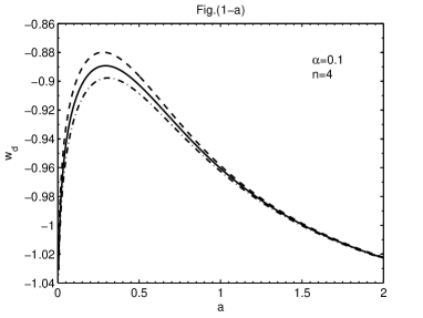
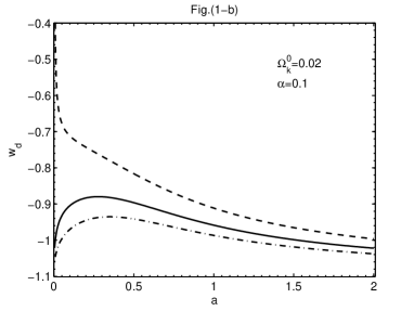
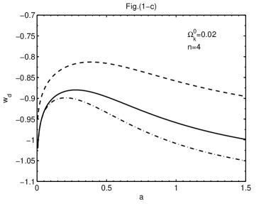
Figure 1: The evolution of EoS parameter, $w_{d}$, versus of $a$ for different model parameters $n$, $\alpha$ and different curvatures $\Omega_{k}$. Fig.(1-a): Dependence of $w_{d}$ on $\Omega_{k}$ , for $n=4$ and $\alpha=0.1$. The dashed, solid and dotted-dashed lines represent the closed, flat and open universe, respectively. Fig.(1-b): the evolution of $w_{d}$ for $n=3$ (dashed line), $n=4$ (solid line) and $n=5$ (dotted-dashed line), by fixing $\alpha=0.1$, in a closed universe . Fig.(1-c): the evolution of $w_{d}$ for $\alpha=0.0$ (dashed line), $\alpha=0.1$ (solid line) and $\alpha=0.15$ (dotted-dashed line) , by fixing $n=4$, in a closed universe.

Fig.(1) shows the evolution of $w_{d}$ of interacting NADE model in terms of scale factor. In Fig.(1-a) we illustrate the evolution of $w_{d}$ for fixed model parameters $n=4$ and $\alpha=0.1$, in open, flat and closed universe. All three cases give the phantom divide at the early time and mimic the cosmological constant at the late time. In Figs.(1-b,1-c), the dependence of the evolution of $w_{d}$ on the model parameters $n$ and $\alpha$ are investigated. Here we choose the closed universe with the present spatial curvature $\Omega_{k0}=0.02$. In Fig.(1-b), by fixing $\alpha=0.1$, we vary the parameter $n$ as 3, 4 and 5. In the case of $n=3$ the interacting NADE model can not cross the phantom divide, while for $n=4$ and $n=5$ the phantom divide can be achieved. In Fig.(1-c) we fix $n=4$ and vary $\alpha$ as $\alpha=0.0$ , $\alpha=0.1$ and eventually $\alpha=0.15$. It can be seen that the phantom divide is archived for $\alpha=0.1$ and $\alpha=0.15$ and it can not be access for $\alpha=0.0$ (the NADE model without interaction).

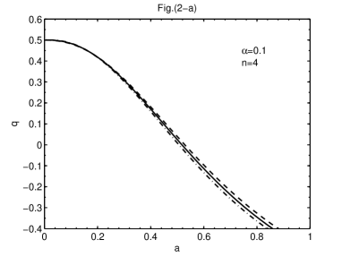
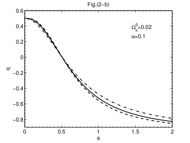
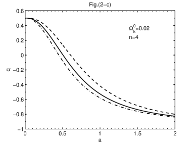
Figure 2: The evolution of $q$ versus of $a$ for different parameters $n$ and $\alpha$ and various contribution of spatial curvatures $\Omega_{k}$. Fig.(2-a): Dependence of $q$ on $\Omega_{k}$ for values $n=4$ and $\alpha=0.1$. The dashed, solid and dotted-dashed lines represent the open, flat and closed universe, respectively. Fig.(2-b): the evolution of $q$ versus $a$, by fixing $\alpha=0.1$, for $n=3$ (dotted-dashed line), $n=4$ (solid line) and $n=5$ (dashed line) in closed universe. Fig.(2-c): the evolution of $q$ versus $a$, by fixing $n=4$, for $\alpha=0.0$ (dotted-dashed line), $\alpha=0.1$ (solid line) and $\alpha=0.15$ (dashed line) in closed universe.

The other cosmological parameter which we demonstrate, is the deceleration parameter $q$. The parameter $q$ in NADE model for non-flat universe is given by Eq.(23). In the early time, where $\Omega_{d}\rightarrow 0$ and $\Omega_{k}\rightarrow 0$, the parameter $q$ converges to $1/2$, whereas the universe has been dominated by dark matter. In Fig(2), we show the evolution of $q$ as a function of cosmic scale factor for different model parameters of NADE model and also for various contribution of spatial curvature of the universe. In Fig.(2-a), the dependence of the evolution of $q$ on the spatial curvature of the universe ($k=0,1,-1$) is sketched for $n=4$ and $\alpha=0.1$. In this model, the deceleration parameter $q$ crosses the boundary $q=0$ from $q>0$ to $q<0$. This implies that the universe undergoes decelerated expansion at the early time and later starts accelerated expansion. The transition from decelerated expansion to the accelerated expansion occurs gradually from closed, flat and open universe. However, the difference between them is very little, but we can interpret that the transition occurs earlier in closed universe. In Figs.(2-b,2-c) the evolution of $q$ in terms of the scale factor is plotted for different values of $n$ and $\alpha$ in the case of closed universe with $\Omega_{k0}=0.02$. In Fig.(2-b), we set $\alpha=0.1$ and change $n$ as 3, 4 and 5. Here the change on the sign of $q$ is taken place at similar $a$ for all values of $n$. It should be noted that in the accelerated universe ($q<0$), the parameter $q$ is smaller for higher values of $n$ while in the decelerated universe ($q>0$), $q$ is larger for higher values of $n$. In Fig.(2-c), by fixing $n=4$, and changing $\alpha$ as $0.0$, $0.1$ and $0.15$ the behavior of $q$ is studied. Here the universe starts accelerated expansion earlier when $\alpha$ is more.

At following, we calculate the evolution trajectories in the statefinder planes and analyze the interacting NADE model in non-flat universe with statefinder point of view. The standard $\Lambda$CDM model in non flat universe corresponds to the fixed point ($s=0$,$r=1+\Omega_{k}$) in the $s-r$ plane Evans . One way to test the ability of a given dark energy model is the deviation value of the model from the fixed point ($s=0$,$r=1+\Omega_{k}$) in $s-r$ diagram. Let us start with Eqs.(33,35 and 34)which describe the evolution of statefinder parameters $r$, $s$ and also $w_{d}^{\prime}$. It is easy to see that in the early time, $w_{d}^{\prime}\rightarrow 0,$ and from ( 34) and(35), $s\rightarrow 0$ and $r\rightarrow 1$. Also it is worth to estimate the values of $\omega_{d}^{\prime}$, $s$ and $r$ at late time when $a\rightarrow\infty$. From Eqs.( 34) and(35), we obtain $s\sim\alpha$ and $r\sim 1$ at late time. So the statefinder parameters ($s$,$r$) reach to the ($\alpha$,$1$) at the late time.

In Fig.(3) the evolution trajectories of statefinder of interacting NADE model with interaction form of $Q_{1}$ is plotted. In Fig.(3-a) , the evolution trajectories is plotted for different closed, flat and open universe for fixed parameters $n=4$ and $\alpha=0.1$. The present values of the statefinder parameters $s_{0}$ and $r_{0}$ is denoted by circle ($s_{0}=0.154$,$r_{0}=0.535$), star ($s_{0}=0.154$,$r_{0}=0.515$) and square ($s_{0}=0.153$,$r_{0}=0.497$) symbols for closed, flat and open universe, respectively. It should be noted that the evolution trajectories start form fixed point ($s=0,r=1$) at the early time, as mentioned above. It can be seen that the different curvatures will lead to different evolutionary behavior in the statefinder plane, starting from the same fixed point ($s=0$,$r=1$) at the early time. The curvature will affect the today’s value of statefinder parameter. Fig.(3-a) shows that the distance to $\Lambda$CDM fixed point in closed universe is shorter than of obtained in flat universe and both of them is shorter than that distance in open universe. Also in closed universe the value of $r$ is the largest, while $s$ is the smallest at present time.

Figs.(3-b & 3-c) indicate the dependence of the evolution trajectories of statefinder diagnostic on $n$ and $\alpha$ in closed universe. Fig.(3-b) shows the influence of the variation of $n$ on the evolution trajectories of statefinder for fixed parameter $\alpha=0.1$. Here the evolution trajectories is calculated for $n=3,4$ and $5$. Symbols on the curves represent the present value of statefinder. The circle indicates ($s_{0}=0.205$,$r_{0}=0.406$) for $n=3$, the star symbol indicates ($s_{0}=0.154$,$r_{0}=0.535$) in the case $n=4$ and the square denotes ($s_{0}=0.123$,$r_{0}=0.620$) for $n=5$. Increasing the parameter $n$ will lead to shorter distance between present values ($s_{0},r_{0}$) and fixed $\Lambda$CDM in this diagram. Also we can see that the higher value of $n$ makes the larger value of $r$ and smaller value of $s$.
In Fig.(3-c), we redo the previous calculation in Fig.(3-b) for fixed parameter $n=4$ and varying parameter $\alpha$ as $0.0$, $0.1$, $0.15$. The variation of $\alpha$ also change the evolution trajectories of statefinder. The present values of statefinder for different values of $\alpha$ are: ($s_{0}=0.162$,$r_{0}=0.564$) for $\alpha=0.0$, ($s_{0}=0.154$ ,$r_{0}=0.535$) for $\alpha=0.1$ and ($s_{0}=0.151$,$r_{0}=0.521$) for $\alpha=0.15$. We can see that the higher value of $\alpha$ makes the smaller value of $r$ and also the smaller value of $s$. It is worth noting that in the case of flat universe, only the parameter $\alpha$ can discriminate the evolution trajectory in $s-r$ plane and the parameter $n$ can only sperate toady’s value of $s$ and $r$(see Figs.(3 & 4) of zhang ). Here in non flat case, both parameters $n$ and $\alpha$ can discriminate the evolution trajectories in $s-r$ plane (see Figs.3-b & 3-c).
At last, we study the interacting NADE model in non flat universe using the $w-w^{\prime}$ analysis. In this analysis, the standard $\Lambda$CDM model corresponds to the fixed point ($w_{d}=-1$,$w_{d}^{\prime}=0$) in the $w-w^{\prime}$ plane. The evolution of $w_{d}$ and $w_{d}^{\prime}$ is given by Eqs.(32, 33). In Fig.(4) the evolution trajectories of $w_{d}^{\prime}$ in $w-w^{\prime}$ plane is shown for different parameters and various curvatures. In Fig.(4-a), we show the evolution trajectories of $w_{d}^{\prime}$ , by fixing the parameters $n=4$ and $\alpha=0.1$ for different spatial curvatures. Here we see that the various spatial curvatures gives the different evolutionary behavior in the $w-w^{\prime}$ plane. The evolution trajectory of different curvatures converges to the fixed point ($w_{d}=-1.1,w_{d}^{\prime}=0.0$) at late time. The present value of $w_{d}$ and $w_{d}^{\prime}$ are: ($w_{d}^{0}=-0.957$,$w_{d}^{\prime 0}=-0.104$) in closed, ($w_{d}^{0}=-0.957$,$w_{d}^{\prime 0}=-0.106$) in flat and ($w_{d}^{0}=-0.957$,$w_{d}^{\prime 0}=-0.107$) in open universe.
In Figs.(4-b, 4-c), the evolution trajectories in $w-w^{\prime}$ plane is discussed for the case of closed universe. In Fig.(4-b), by fixing $\alpha=0.1$, we vary the parameter $n$ as $3,4$ and $5$. The today’s value of $w_{d}^{0},w_{d}^{\prime 0}$ is denoted by symbols on the lines. The circle symbol shows the present value ($w_{d}^{0}=-0.910,w_{d}^{\prime 0}=-0.142$) in the case of $n=3$, star ($w_{d}^{0}=-0.957,w_{d}^{\prime 0}=-0.104$) for $n=4$ and square ($w_{d}^{0}=-0.986,w_{d}^{\prime 0}=0-0.082$) for $n=5$. Increasing the parameter $n$ will lead to closing the present values of $w_{d}^{0},w_{d}^{\prime 0}$ tend to the fixed point ($-1,0$) in $w-w^{\prime}$ plane. The higher value of $n$ obtains the smaller values of $w_{d}$ and the bigger value of $w^{\prime}$.
In Fig.(4-c), we fix $n=4$ and vary $\alpha$ as $0.0,0.1$ and $0.15$. The present values of $w_{d}^{0},w_{d}^{\prime 0}$ are shown by symbols on the lines. The circle symbol indicates the present value ($w_{d}^{0}=-0.857,w_{d}^{\prime 0}=0.051$) in the case of $\alpha=0.0$, the star shows ($w_{d}^{0}=-0.959,w_{d}^{\prime 0}=0.035$) for $\alpha=0.1$ and the square represents ($w_{d}^{0}=-1.01,w_{d}^{\prime 0}=0.027$) for $\alpha=0.15$. Increasing the interaction parameter $\alpha$ would lead to decreasing the present value ($w^{0},w^{\prime 0}$) in $w-w^{\prime}$ plane.

V Conclusion

In this work, the interacting NADE model in non-flat universe has been given. We studied the effect of spatial curvature $\Omega_{k}$, interaction coefficient $\alpha$ and the main parameter of NADE, $n$, On EoS parameter $w_{d}$ and deceleration parameter $q$. We showed that in the early and present time for $\alpha_{1}=0.1,$ the phantom divide is not available for $n=3$ and it is achieved for $n\geq 4$. By increasing $n$ and $\alpha$ in a closed universe, the trend of $w_{d}$ decreases. We obtained a minimum value for $n$ in both early and present time, in order to that the NADE model crosses the phantom divide. It was shown that the treatment of both parameter $w_{d}$ and $q$ are dependent on the type of spatial curvature. At last, we investigated the interacting NADE model in a non-flat universe by means of statefinder diagnostic and $w-w^{\prime}$ analysis viewpoints. Here we showed that the spatial curvature can affect the evolution trajectories in ($s,r$) and ($w_{d},w_{d}^{\prime}$) planes. Also the trajectories in these planes can be affected by the model parameters of interacting NADE, $n$ and $\alpha$. In non flat universe, the statefinder trajectory is discriminated by both $n$ and $\alpha$. It should be noted that in the case of flat universe, only the parameter $\alpha$ can discriminate the evolution trajectory in $s-r$ plane and $n$ can only discriminate toady’s value of $s$ and $r$(see Figs.(3 & 4) of zhang ). While in non flat universe, both parameteres $n$ and $\alpha$ in addition to discrimination of {$s,r$} at present time, can discriminate the evolution trajectory in $s-r$ plane (see Figs.3-b & 3-c). It is worthwhile to mention that all computations is reduced to previous work in the limiting case of flat universe zhang .

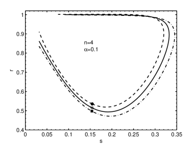
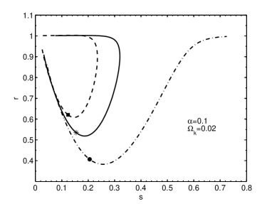
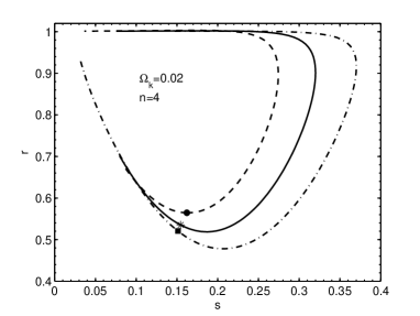
Figure 3: Fig.(3-a): Evolution trajectories of the statefinder in the $r-s$ plane for open (dotted-dashed line), flat (solid line) and closed universe (dashed line). Square, circle and star symbols on the curves are the today’s values of the statefinder parameters ($s_{0}$,$r_{0}$). Here the model parameters are $n=4$ and $\alpha=0.1$.
Fig.(3-b): Evolution trajectories of the statefinder in the $r-s$ plane for different values of $n$ as 3 (dotted-dashed line), 4 (solid line) and 5 (dashed line) , by fixing $\alpha=0.1$ in closed universe. Fig.(3-c): Evolution trajectories of the statefinder in the $r-s$ plane for different values of $\alpha$ as $0.0$ (dotted-dashed line),$0.1$ (solid line) and $0.15$ (dashed line) , by fixing $n=4$ in closed universe.

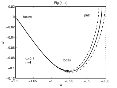
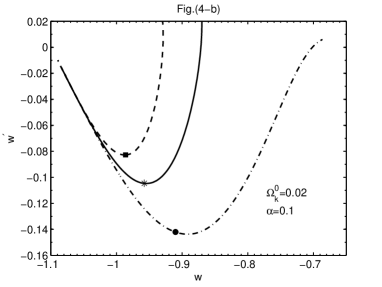
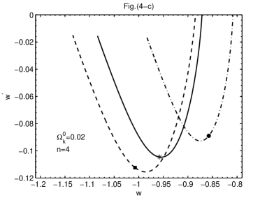
Figure 4: Fig.(4-a): the evolution trajectories in $w_{d},w^{\prime}_{d}$ plane, by fixing $n=4$ and $\alpha=0.1$, for closed (dashed line), flat (solid line) and open universe (dotted-dashed line). The present value of $w_{d}^{0},w^{\prime 0}_{d}$ is indicated by symbols on the curves. Fig.(4-b): Evolution trajectories in $w_{d},w^{\prime}_{d}$ plane for different values of $n$ as 3 (dotted-dashed line), 4 (solid line) and 5 (dashed line) , by fixing $\alpha=0.1$ in closed universe. Fig.(4-c): Evolution trajectories in $w_{d},w^{\prime}_{d}$ plane for different values of $\alpha$ as $0.0$ (dotted-dashed line), $0.1$ (solid line) and $0.15$ (dashed line) , by fixing $n=4$ in closed universe.

References

-
(1)
A. G. Riess et al. [Supernova Search Team
Collaboration], Astron. J. 116, 1009 (1998);
S. Perlmutter et al. [Supernova Cosmology Project Collaboration], Astrophys. J. 517, 565 (1999);
P. Astier et al., Astron. Astrophys. 447, 31 (2006).
-
(2)
M. Tegmark et al. [SDSS Collaboration], Phys. Rev. D 69, 103501 (2004);
K. Abazajian et al. [SDSS Collaboration], Astron. J. 128, 502 (2004);
K. Abazajian et al. [SDSS Collaboration], Astron. J. 129, 1755 (2005).
-
(3)
D. N. Spergel et al. [WMAP Collaboration],Astrophys. J. Suppl. 148, 175 (2003);
D. N. Spergel et al., Astrophys.J.Suppl. 170, 377 (2007);
-
(4)
T. Padmanabhan, Phys. Rep. 380, 235 (2003);
P. J. E. Peebles, B. Ratra, Rev. Mod. Phys. 75, 559 (2003);
E. J. Copeland, M. Sami and S. Tsujikawa, Int.J.Mod.Phys.D 15, 1753 (2006). -
(5)
P. Horava, D. Minic, Phys. Rev. Lett. 85, 1610 (2000);
P. Horava, D. Minic, Phys. Rev. Lett. 509 138 (2001);
K. Enqvist, M. S. Sloth, Phys. Rev. Lett. 93 221302 (2004);
S. D. H. Hsu, Phys. Lett. B 594, 13 (2004);
M. R. Setare, S. Shafei, JCAP 09, 011 (2006);
M. R. Setare, Phys. Lett. B 644, 99 (2007);
M. R. Setare, E. C. Vagenas, Phys. Lett. B 666, 111 (2008);
M. R. Setare, Phys. Lett. B 642, 421 (2006);
H. M. Sadjadi, Eur.Phys.J.C 62, 419,(2009);
B. Wang, C. Y. Lin and E. Abdalla, Phys. Lett. B 637,357 (2005);
M. R. Setare, Eur. Phys. J. C 52,689 (2007);
Bin Wang, et al., Nucl.Phys.B 778, 69 (2007). - (6) R. G. Cai, Phys. Lett. B 657, 228 (2007).
- (7) E. J. Copeland, M. Sami, S. Tsujikawa, Int. J. Mod. Phys. D 15, 1753 (2006).
-
(8)
M. Maziashvili Int. J. Mod. Phys. D 16, 1531 (2007);
M. Maziashvili, Phys. Lett. B 652, 165 (2007). -
(9)
R. G. Cai, Phys. Lett. B 657, 228 (2007).
-
(10)
H. Wei & R. G. Cai, Phys. Rev. D 71, 043504 (2005);
H. Wei & S. N. Zhang, Phys. Lett. B 644, 7 (2007);
A. Sheykhi, Phys. Rev. D 81, 023525 (2010).
- (11) O. Bertolami, F. Gil Pedro, Le Delliou, M., Phys. Lett. B 654, 165 (2007).
- (12) C. Feng, B. Wang, Y. Gong, R. K. Su, J. Cosmol. Astropart. Phys. 0709, 005 (2007).
-
(13)
A. Sheykhi, Phys. Lett. B 680, 113 (2009).
-
(14)
M. R. Setare, JCAB, 0701, 023 (2007);
K. Karami, J. Fehri, Phys. Lett. B 684, 61 (2010).
-
(15)
J. L. Sievers, et al., Astrophys. J. 591, 599 (2003);
C.B. Netterfield, et al., Astrophys. J. 571, 604 (2002);
A. Benoit, et al., Astron. Astrophys. 399, L25 (2003);
A. Benoit, et al., Astron. Astrophys. 399, L19 (2003). -
(16)
R. R. Caldwell, M. Kamionkowski, JCAP 0409, 009 (2004);
B. Wang, Y. G. Gong, R. K. Su, Phys. Lett. B 605, 9 (2005). -
(17)
H. Wei & R. G. Cai, Phys. Lett. B 660, 113 (2008).
- (18) H. Wei, R. G. Cai, Phys. Lett. B 655, 1 (2007).
-
(19)
L. Zhang, J. Cui, J. Zhang & X. Zhang, Int. J. Mod. Phys. D
19, 21 (2010).
-
(20)
V. Sahni, T. D. Saini, A. A. Starobinsky and U. Alam, JETP
Lett. 77, 201 (2003);
U. Alam, V. Sahni, T. D. Saini and A. A. Starobinsky, Mon. Not. Roy. Astron. Soc. 344, 1057 (2003). - (21) V. Sahni, T. D. Saini, A. A. Starobinsky and U. Alam, JETP Lett. 77, 201 (2003).
- (22) U. Alam, V. Sahni, T. D. Saini and A. A. Starobinsky, Mon. Not. Roy. Astron. Soc. 344, 1057 (2003).
- (23) W. Zimdahl and D. Pavon, Gen. Rel. Grav. 36, 1483 (2004).
- (24) X. Zhang, Phys. Lett. B 611, 1 (2005).
- (25) X. Zhang, Int. J. Mod. Phys. D 14, 1597 (2005).
- (26) J. Zhang, X. Zhang and H. Liu, Phys.Lett.B 659, 26 (2008).
- (27) M. R. Setare, J. Zhang and X. Zhang, JCAP 0703, 007 (2007).
- (28) B. R. Chang, H. Y. Liu, L. X. Xu, C. W. Zhang and Y. L. Ping, JCAP 0701, 016 (2007).
- (29) Y. Shao and Y. Gui, Mod.Phys.Lett.A 23, 65 (2008).
-
(30)
R. J. Scherrer, Phys. Rev. D 73, 043502
(2006);
T. Chiba, Phys. Rev. D 73, 063501 (2006);
V. Barger, E. Guarnaccia and D. Marfatia, Phys. Lett. B 635, 61 (2006);
W. Zhao, Phys. Rev. D 73, 123509 (2006);
W. Zhao, Phys.Lett.B 655, 97 (2007);
G. Calcagni and A. R. Liddle, Phys. Rev. D 74, 043528 (2006);
Z. K. Guo, Y. S. Piao, X. M. Zhang and Y. Z. Zhang, Phys. Rev. D 74, 127304 (2006);
Z. G. Huang, H. Q. Lu and W. Fang, Int.J.Mod.Phys.D 16, 1109 (2007);
Z. G. Huang, X. H. Li and Q. Q. Sun, Astrophys. Space Sci. 310, 53 (2007);
R. de Putter and E. V. Linder, Astropart.Phys. 28 263 (2007).
-
(31)
C. L. Bennett, et al., ApJ. Suppl. 148, 1 (2003);
D. N. Spergel, ApJ. Suppl. 148, 175 (2003). - (32) A. K. D. Evans, I. K. Wehus, O. Gron and O. Elgaroy, Astron. Astrophys. 430, 399 (2005).