Energy dependence of nucleon-nucleon potentials in lattice QCD

Abstract:

Recently a new approach to calculate the nuclear potential from lattice QCD has been proposed. In the approach the nuclear potential is constructed from Bethe-Salpeter (BS) wave functons through the Schröedinger equation. The procedure leads to non-local but energy independent potential, which can be expanded in terms of local functions. In several recent applications of this method, local potentials, which correspond to the leading order (LO) terms of the expansion, are calculated from the BS wave function at $E\simeq 0$ MeV, where $E$ is the center of mass energy. It is therefore important to check the validity of the LO approximation obtained at $E\simeq 0$. In this report, in order to check how well the LO approximation for the NN potentials works, we compare the LO potentials determined from the BS wave function at $E\simeq 45$ MeV with those at $E\simeq 0$ MeV in quenched QCD. We find that the difference of the LO potentials between two energies are not found wihin the statistical errors. This shows that the LO approximation for the potential is valid at low energies to describe the NN interactions.

1 Introduction

The nucleon-nucleon (NN) potential is widely used in nuclear physics. Once the NN potential is known, one can, in principle, determine various structure of nuclei, by simply solving the corresponding Schrödinger equation. In the past few decades, several different NN potentials, such as phenomenological potentials determined from the fit of NN scattering data with $\chi^{2}/{\rm dof}\sim 1$ at $T_{\rm lab}<300$ MeV [1, 2, 3] or potentials based on effective field theory [4], have been proposed. Although these potentials can reproduce the scattering data to a quite good accuracy, they have a drawback that they need a large number of parameters to describe the phase shift of the NN scattering ($\mbox{AV}_{18}$ needs 40 and ChPT in $\mbox{N}^{3}$LO needs 24 parameters. ). In this respect, the NN potential from Lattice QCD proposed in Ref. [5, 6, 7] has an advantage: It requires only a few fundamental parameters of QCD, the gauge coupling constant $g^{2}$ and quark masses $m_{u},m_{d},m_{s},\cdots$, so that the method can be also applied to hyperon systems ($N\Lambda$,$N\Sigma$ …) [8], for which only a limited number of experimental information is obtained so far.

Recently Hadrons to Atomic nuclei from Lattice (HAL) QCD collaboration is formed to study various aspect of baryon-baryon potentials based on the first principle of QCD. In the approach by the HAL QCD collaboration, the non-local but energy-independent potential $U(r,r^{\prime})$ is first constructed from the Bethe-Salpeter (BS) wave function via the Schrödinger equation [5, 6, 7]. The non-local potential $U(r,r^{\prime})$ can be described in terms of local functions using the derivative expansion, whose leading order contribution gives the local potential. In several applications of this method, the leading order local potentials have been evaluated at zero energy in the center of mass frame. Therefore, in practice, it is important to know at which energy range the leading order local potential is accurate enough to approximate the non-local potential $U(r,r^{\prime})$, which is faithful to the scattering data by construction. In this report, we extract the leading order local potentials at non-zero energy from the quenched lattice QCD simulation, and compare them with those previously obtained at zero energy. A difference between them gives an estimate of higher order correction in the derivative expansion.

This report is organized as follows. In section 2, we give a brief review of the method to extract the NN potential in Lattice QCD using the derivative expansion. In section 3, we compare the leading local potentials between zero and non-zero energies. We have found that a difference between them is small compared to statistical errors. In section 4. we consider contaminations to the potentials from excited states, which become manifest at large separation where the potential is expected to vanish. Section 5 is devoted to summary and conclusion.

2 NN potential from Lattice QCD

The non-local potential $U(\vec{r},\vec{r}^{\prime})$ is constructed from the equal-time Bethe-Salpeter (BS) wave function $\phi(\vec{x},k)$ through the Shrödinger equation [6, 7] as

$$\left(\triangle+k^{2}\right)\ \phi(\vec{r};k)=m_{N}\int d^{3}\ r^{\prime}\ U(\vec{r},\vec{r}^{\prime})\ \phi(\vec{r}^{\prime},k),$$ (1)

where ”$k$” denotes the “asymptotic momentum”, which is related to the total relativistic energy $W$ as $W=2\sqrt{m^{2}_{N}+k^{2}}$. The derivative expansion up to $\vec{\nabla}$, together with various constraints from symmetries leads to the conventional form of the NN potential at low energies widely used in nuclear physics [9]:

$$U(\vec{r},\vec{r}^{\prime})=\left[V_{0}^{I}(r)+V_{\sigma}^{I}(r)\ \left(\sigma_{1}\cdot\sigma_{2}\right)+V_{T}^{I}(r)\ S_{12}+V_{LS}^{I}(x)\ \vec{L}\cdot\vec{S}+\mathcal{O}(\vec{\nabla^{2}})\right]\delta(\vec{r}-\vec{r}^{\prime}),$$ (2)

where $r=|\vec{r}|$, $S_{12}=3(\vec{\sigma_{1}\cdot\vec{r}})(\vec{\sigma_{2}}\cdot\vec{r})/r^{2}-\vec{\sigma_{1}}\cdot\vec{\sigma_{2}}$ is the tensor operator, $\vec{S}=\left(\vec{\sigma_{1}}+\vec{\sigma_{2}}\right)/2$ is the total spin, $\vec{L}=\vec{r}\times\vec{p}$ is the orbital angular momentum, and $I=0,1$ is the total isospin. Note that $\vec{L}\cdot\vec{S}$, which is $\mathcal{O}(\vec{\nabla})$, is of next-to-leading order in the expansion. Eq. (1) with (2) successively determines local functions $V^{I}_{A}(x)$ ($A=0,\sigma,T,LS,\cdots$).

The BS wave function on the lattice with the lattice size $L$ is defined by

$$\phi^{S}(\vec{r};k)=\frac{1}{L^{3}}\displaystyle\sum_{\vec{x}}P^{S}_{\alpha\beta}\langle 0|\hat{n}_{\beta}\left(\vec{r}+\vec{x}\right)\hat{p}_{\alpha}(\vec{x})|B=2;W\rangle,\hskip 28.45274ptW=2\sqrt{m_{N}^{2}+k^{2}},$$ (3)

where $W$ is the total energy of the two nucleon system in the center of mass system, and $P^{\sigma}_{\alpha\beta}$ denotes a projection operator to the spin singlet state ($P^{S=0}_{\alpha,\beta}=(\sigma_{2})_{\alpha,\beta}$) or triplet state ($P^{S=1}_{\alpha,\beta}=(\sigma_{1})_{\alpha,\beta}$) for spinor indices $\alpha$ and $\beta$. Local composite operators for the proton and the neutron $\hat{n}$ and $\hat{p}$ are given by

$$\hat{n}_{\beta}(y) = \epsilon_{abc}\left(\hat{u}_{\alpha}(y)C\gamma_{5}\hat{d}_{b}(y)\right)\hat{d}_{c\beta}(y),\hskip 28.45274pt\hat{p}_{\alpha}(x)=\epsilon_{abc}\left(\hat{u}_{\alpha}(x)C\gamma_{5}\hat{d}_{b}(x)\right)\hat{u}_{c\alpha}(x),$$ (4)

where, $a,b,c$ denote color indices, and $C$ is the charge conjugation matrix.

In this report, we consider potentials for the ${}^{1}S_{0}$ state and the ${}^{3}S_{1}$ – ${}^{3}D_{1}$ state. In the case of ${}^{1}S_{0}$ state, the Schrödinger equation at leading order becomes

$$(\triangle+k^{2})\phi^{{}^{1}S_{0}}(r;k)=2\mu V^{{}^{1}S_{0}}(r)\phi^{{}^{1}S_{0}}(r;k)$$ (5)

for the spin singlet channel ($S=0$) with the reduced mass $\mu=m_{N}/2$, where the wave function $\phi^{{}^{1}S_{0}}(r;k)$ for the ${}^{1}S_{0}$ state is given by the projection $P$ as

$$\phi^{{}^{1}S_{0}}(r;k) = P\phi^{0}(\vec{r};k)\equiv\frac{1}{24}\displaystyle\sum_{R\in O}\phi^{0}(R[\vec{r}];k).$$ (6)

Here the summation over $R\in O$ is taken for the cubic transformation group to project out the $A_{1}^{+}$ state. Then the central potential is easily obtained as

$$V^{{}^{1}S_{0}}(r) \equiv V_{0}^{1}(r)-3V_{\sigma}^{1}(r)=E+\frac{1}{2\mu}\frac{\triangle\phi^{{}^{1}S_{0}}(r;k)}{\phi^{{}^{1}S_{0}}(r;k)},$$ (7)

where $E(=\frac{k^{2}}{2\mu})$ is an effective kinetic energy in the center of mass system.

For the spin triplet channel ($S=1$), the Schrödinger equation at leading order becomes more complicated due to the mixing between ${}^{3}S_{1}$ and ${}^{3}D_{1}$ components by the tensor potential:

$$(\triangle+k^{2})\phi^{1}(\vec{r};k) = 2\mu\{V_{c}(r)+V_{T}(r)S_{12}\}\phi^{1}(\vec{r};k)$$ (8)

where $V_{c}(r)\equiv V_{0}^{0}(r)+V_{\sigma}^{0}(r)$. By two projections $P$ and $Q\equiv 1-P$, the above Schrödinger equation is decomposed as

$$\left(\begin{array}[]{cc}P\phi^{1}(\vec{r};k)&PS_{12}\phi^{1}(\vec{r};k)\\ Q\phi^{1}(\vec{r};k)&QS_{12}\phi^{1}(\vec{r};k)\\ \end{array}\right)\left(\begin{array}[]{c}V_{c}(r)\\ V_{T}(r)\\ \end{array}\right) = \frac{\triangle+k^{2}}{2\mu}\left(\begin{array}[]{c}P\phi^{1}(\vec{r};k)\\ Q\phi^{1}(\vec{r};k)\\ \end{array}\right),$$ (15)

from which $V_{c}(r)$ and $V_{T}(r)$ can be separately obtained[10, 7].

3 Numerical Simulations and results

3.1 Lattice QCD setup

We employ the standard plaquette gauge action on a $32^{3}\times 48$ lattice with the $\beta=5.7$ for quenched gauge configurations. Quark propagators are calculated by the Wilson quark action at $\kappa=0.1665$. This setup leads to the lattice spacing $a^{-1}=1.44(2)$ GeV ($a\sim 0.137$ fm) from $m_{\rho}$, the spatial extension $L=32a\sim 4.4$ fm, $m_{\pi}\sim 0.53$ GeV and $m_{N}\sim 1.33$ GeV [11]. Quenched gauge configurations are generated by the heatbath algorithm with overrelaxation. Potentials are measured on configurations separated by 200 sweep. 4000 configurations are accumulated to obtain results in this report. These calculations are performed on Blue Gene/L at KEK.

The BS wave function is obtained from the four-point correlator of nucleon operators in the large $t$ region,

$$G^{(4)}(\vec{x},\vec{y},t,t_{0}) = \langle 0|\hat{n}_{\beta}(\vec{y},t)\hat{p}_{\alpha}(\vec{x},t)\bar{\mathcal{J}}_{pn}(t_{0})|0\rangle=\sum_{n}A_{n}\langle 0|\hat{n}_{\beta}(\vec{y})\hat{p}_{\alpha}(\vec{x})|B=2;W_{n}\rangle e^{-W_{n}(t-t_{0})}$$ (16)

$$\sim A_{0}\langle 0|\hat{n}_{\beta}(\vec{y})\hat{p}_{\alpha}(\vec{x})|B=2;W_{0}\rangle e^{-W_{0}(t-t_{0})},\hskip 28.45274ptW_{n}=2\sqrt{m_{N}^{2}+k_{n}^{2}}.$$

Here the source located at $t=t_{0}$, $\bar{\mathcal{J}}_{pn}(t_{0})$, is defined by

$$\bar{\mathcal{J}}_{pn}=P^{S}_{\alpha^{\prime}\beta^{\prime}}\bar{P}_{\alpha^{\prime}}(t_{0})\bar{N}_{\beta^{\prime}}(t_{0}),\hskip 28.45274pt\bar{P}_{\alpha}\equiv\epsilon_{a,b,c}\left(\bar{U}_{a}C\gamma_{5}\bar{D}_{b}\right)\bar{U}_{c\alpha},\hskip 14.22636pt\bar{N}_{\beta}\equiv\epsilon_{a,b,c}\left(\bar{U}_{a}C\gamma_{5}\bar{D}_{b}\right)\bar{D}_{c\beta},$$

where

$$U(t) = \sum_{\vec{x}}u(t,\vec{x})f(\vec{x}),\hskip 28.45274ptD(t)=\sum_{\vec{x}}d(t,\vec{x})f(\vec{x}),$$ (17)

where $f(x)$ is source function, as will be seen later. By examining the $t$ dependence of potentials, we see that ground state saturations for potentials are achieved at $t-t_{0}=9$.

3.2 Periodic and anti periodic boundary conditions

The periodic boundary condition (PBC) is imposed on the quark fields along the spatial directions to obtain the NN potential at $E\sim 0$ MeV, while the anti-periodic boundary condition (APBC) is employed for the NN potential at $E\sim 3\times(\pi/L)^{2}/m_{N}$, which corresponds to $45$ MeV in the center of mass system. For the PBC, we employ the wall source, i.e., $f(\vec{x})=1$ , which enhance ground state of PBC, $\vec{p}=(0,0,0)\pi/L$. On the other hand, for the APBC, we employ four types of momentum wall sources, $f(\vec{x})=\cos((+x+y+z)\pi/L)$, $\cos((-x+y+z)\pi/L)$, $\cos((+x-y+z)\pi/L)$, and $\cos((-x-y+z)\pi/L)$, where these sources enhance the ground state of APBC, i.e., $\vec{p}=(1,1,1)\pi/L$ state. Here, we have imposed positive parity to the system by using the wall source with a cosine type instead of an exponential type. After the summation over the results of four sources, the $A_{1}^{+}$ representation is obtained. To improve the statistics for the PBC case, we locate four sources on different time slices on each configuration.

To evaluate the central potential by eq. (7), we need to determine the first term, $k^{2}/2\mu$, which, in principle, is obtained through the relation $W_{0}=2\sqrt{m_{N}^{2}+k^{2}}$. Within statistical and systematic errors, however, the values of $k^{2}$ turn out to be close to the free values. We therefore adopt the free values, $E=k^{2}/m_{N}=0$ MeV (PBC) and $E=k^{2}/m_{N}=3(\pi/L)^{2}/m_{N}=45$ MeV (APBC), to calculate potentials in this report.

3.3 Comparison of local potentials between two energies

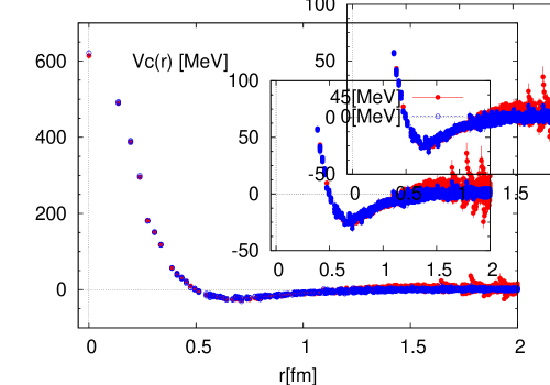
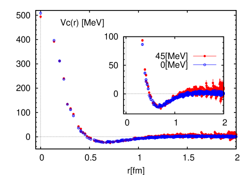
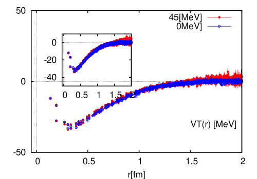
Figure 1: Comparison of local potentials with the PBC (blue open circle) and the APBC (red closed circle) at $t-t_{0}=9$ and $r\leq 2.0$ fm. The left figure shows the ${}^{1}S_{0}$ central potential, while the center and the right represent the ${}^{3}S_{1}-^{3}D_{1}$ central and tensor potentials, respectively.

In Figure 1, we compare potentials at the leading order of the derivative expansion obtained at $E\simeq 45$ MeV (red circles) with those at $E\simeq 0$ MeV (blue circles), for the $V^{{}^{1}S_{0}}(r)$ (the left), $V_{c}(r)$ (the center) and $V_{T}(r)$ (the right). All data are taken at $t-t_{0}=9$, where grand state saturations for the potentials are achieved. From these figures we observe that the agreement of potentials between two energies is quite good for all cases within the statistical errors. We therefore conclude that the leading order contribution in the derivative expansion gives a very accurate approximation for the energy-independent non-local potential $U(\vec{r},\vec{r}^{\prime})$ in the energy range from $E=0$ MeV to $E=45$ MeV, in the case of the quenched approximation at $m_{\pi}\simeq 530$ MeV. Note that the NLO contribution is absent for the spin-singlet channel while the NLO $V_{LS}$ potential exists for the spin-triplet. The agreement of $V_{c}$ and $V_{T}$ between two energies suggests that $V_{LS}(r)$ is sufficiently small below $E=45$ MeV, at least for $m_{\pi}\simeq 530$ MeV.

4 Contamination from excited states at large distances

Results in the previous section show that the local potentials obtained from the BS wave function at $E\simeq 45$ MeV agree well with those at $E\simeq 0$ MeV. One may notice, however, that potentials obtained at $E\simeq 45$ MeV (APBC) deviate from zero at large $r$, where potentials are expected to vanish. These deviations are not statistical fluctuations , as seen in Fig.2, where the local potentials obtained with the APBC are plotted as a function of $r$ at $t-t_{0}=3,6,9$: Deviations of the potentials from zero at large distances have characteristic structures, which are most clearly seen at $t-t_{0}=3$, and the deviations decrease as $t-t_{0}$ increases. These observations suggests that the deviations of the potential from zero are caused by contaminations of excited states.

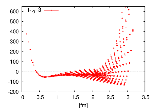
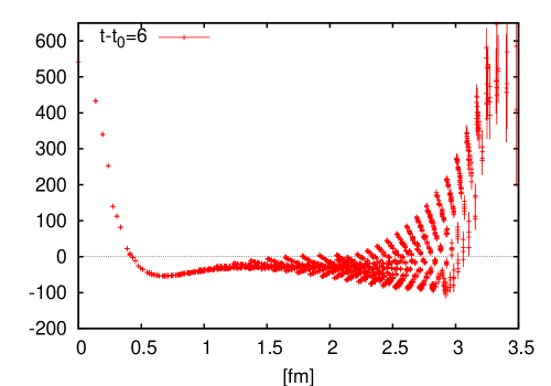
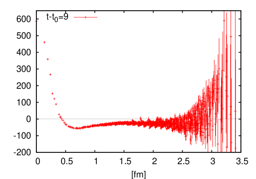
Figure 2: These figures are ${}^{1}S_{0}$ central potential with the APBC at $t-t_{0}=3$ (left), $6$ (center) and $9$ (right). These potential deviate from zero at $r>2$ fm. Deviations of potentials are decrease as $t-t_{0}$ increases.

Here we discuss how contaminations of excited states to the BS wave function affects the form of the corresponding potential. Let us assume that the BS wave function extracted from the 4 point function is dominated by the grand state with a small contamination of one excited state as follows.

$$\phi(\vec{r},t)=\psi(\vec{r},k_{0})\ e^{-W_{0}\ t}+\psi(\vec{r},k_{1})\ e^{-W_{1}\ t},\hskip 28.45274pt(k_{0}<k_{1}),$$ (18)

where $W_{n}=2\sqrt{m_{N}^{2}+k_{n}^{2}}$, and $\psi(\vec{r},k_{0})$ is the BS wave function of the grand state with $E_{0}=k_{0}^{2}/m_{N}$ while $\psi(\vec{r},k_{1})$ is the wave function of the excited state with $E_{1}=k_{1}^{2}/m_{N}$. At sufficiently large $r$, we assume that both wave function satisfy

$$\frac{1}{m_{N}}(\Delta+k_{0}^{2})\ \psi(\vec{r},k_{0})=0$$ (19)

$$\frac{1}{m_{N}}(\Delta+k_{1}^{2})\ \psi(\vec{r},k_{1})=0.$$ (20)

By inserting eq. (18) into eq. (7), we arrive at the following expression:

$$V_{\rm mix}(\vec{r}) = \frac{1}{m_{N}}\frac{\Delta\phi(\vec{r},t)}{\phi(\vec{r},t)}+\frac{k_{0}^{2}}{m_{N}}\stackrel{{\scriptstyle r\rightarrow\infty}}{{\longrightarrow}}\frac{1}{m_{N}}\left(k^{2}_{1}-k^{2}_{0}\right)\ P(\vec{r}),$$ (21)

where $P(\vec{r})$ is given by

$$P(\vec{r})=\frac{\psi(\vec{r},k_{1})}{\psi(\vec{r},k_{0})+\psi(\vec{r},k_{1})e^{-t(W_{1}-W_{0})}}e^{-t(W_{1}-W_{0})}.$$ (22)

We see that, even in the non-interacting region where the true potential $V(\vec{r})$ vanishes, eq (21) leads to a non-vanishing ”potential” as

$$V_{\rm mix}(\vec{r})=\frac{k_{1}^{2}-k_{0}^{2}}{m_{N}}P(\vec{r})\neq 0.$$ (23)

The agreement of local potentials between two energies indicates that the effect of these contaminations to potentials is smaller than statistical errors at short distance ($r<2.0$ fm). Therefore the conclusion in the previous section remains true. Since the true potentials vanish at long distance, however, the small effect due to the contaminations can become significant. Note that the APBC implies that not only the numerator but also the denominator of $P(\vec{r})$ vanish at boundaries, so that $P(\vec{r})$ could become large near boundaries. The consideration so far suggests that the deviations of the potentials from zero with the APBC at large $r$ is caused by the contaminations from the excited states. Our choices of momentum wall sources creates not only the grand state with $\vec{p}=\frac{\pi}{L}(\pm 1,\pm 1,\pm 1)$ but also the excited state with $\vec{p}=\frac{\pi}{L}(\pm 3,\pm 3,\pm 3)$. Moreover the energy difference in lattice unit is not so large: $W_{1}-W_{0}\simeq 0.23/a$ ($\sim 360$ MeV) in this case. Therefore it is likely that the contamination comes from the $(3,3,3)$ excited state. This observation, however, needs to be confirmed, which is now underway.

5 Summary and conclusion

We have examined how well the leading order contributions in the derivative expansion of the non-local potential $U(r,r^{\prime})$ describe the NN interactions in the wide range of energy. We have compared the local NN potentials for the ${}^{1}S_{0}$ state (the central potential) and for the ${}^{3}S_{1}$–${}^{3}D_{1}$ state (the central and the tensor potentials) obtained at $\simeq 45$ MeV with those obtained at $E\simeq 0$ MeV in quenched QCD at $m_{\pi}\simeq 530$ MeV. We have found that differences of these potentials between two energies are very small. From this result we conclude that the leading order local potentials in the derivative expansion are good approximations for the NN potentials at energy up to 45 MeV in quenched QCD, and that the local potential constructed at $E\sim 0$ MeV can be used to investigate properties of the NN interaction at low energy.

In the future it is important to apply the analysis in this report to the NN potentials in full QCD at lighter pion mass and to more general potentials including hyperons, in order to confirm the validity of the leading order local potential approximation for these cases.

Acknoendwledgments

We are grateful for authors and maintainers of CPS++[12], of which a modified version is used for simulations done in this work. This work is supported by the Large Scale Simulation Program No.08-19(FY2008) and No.09-23(FY2009) of High Energy Accelerator Research Organization (KEK). This work was supported in part by the Grant-in-Aid of the Ministry of Education, Science and Technology, Sports and Culture (Nos. 20340047, 20105001, 20105003).

References

- [1] R. Machleidt, Phys. Rev. C 63, 024001 (2001)
- [2] R. B. Wiringa, V. G. J. Stoks and R. Schiavilla, Phys. Rev. C 51, 38 (1995)
- [3] V. G. J. Stoks, R. A. M. Klomp, C. P. F. Terheggen and J. J. de Swart, Phys. Rev. C 49, 2950 (1994)
- [4] S. Weinberg, Phys. Lett. B 251, 288 (1990).
- [5] N. Ishii, S. Aoki and T. Hatsuda, Phys. Rev. Lett. 99, 022001 (2007)
- [6] S. Aoki, T. Hatsuda and N. Ishii, Comput. Sci. Dis. 1, 015009 (2008)
- [7] S. Aoki, T. Hatsuda and N. Ishii, arXiv:0909.5585 [hep-lat].
- [8] H. Nemura, N. Ishii, S. Aoki and T. Hatsuda, Phys. Lett. B 673, 136 (2009)
- [9] S.Okubo and R.E.Marshak, Ann. Phys.(NY) 4, 166 (1958)
- [10] N. Ishii, S. Aoki and T. Hatsuda, arXiv:0903.5497 [hep-lat].
- [11] M. Fukugita, Y. Kuramashi, M. Okawa, H. Mino and A. Ukawa, Phys. Rev. D 52, 3003 (1995)
-
[12]
CPS++
http://qcdoc.phys.columbia.edu/cps.html(maintainer: Chulwoo Jung).