Constructing semi-empirical sunspot models for helioseismology

Abstract

One goal of helioseismology is to determine the subsurface structure of sunspots. In order to do so, it is important to understand first the near-surface effects of sunspots on solar waves, which are dominant. Here we construct simplified, cylindrically-symmetric sunspot models, which are designed to capture the magnetic and thermodynamics effects coming from about 500 km below the quiet-Sun $\tau_{5000}=1$ level to the lower chromosphere. We use a combination of existing semi-empirical models of sunspot thermodynamic structure (density, temperature, pressure): the umbral model of Maltby et al. (1986) and the penumbral model of Ding and Fang (1989). The OPAL equation of state tables are used to derive the sound speed profile. We smoothly merge the near-surface properties to the quiet-Sun values about 1 Mm below the surface. The umbral and penumbral radii are free parameters. The magnetic field is added to the thermodynamic structure, without requiring magnetostatic equilibrium. The vertical component of the magnetic field is assumed to have a Gaussian horizontal profile, with a maximum surface field strength fixed by surface observations. The full magnetic field vector is solenoidal and determined by the on-axis vertical field, which, at the surface, is chosen such that the field inclination is 45^∘ at the umbral-penumbral boundary. We construct a particular sunspot model based on SOHO/MDI observations of the sunspot in active region NOAA 9787. The helioseismic signature of the model sunspot is studied using numerical simulations of the propagation of f, p₁, and p₂ wave packets. These simulations are compared against cross-covariances of the observed wave field. We find that the sunspot model gives a helioseismic signature that is similar to the observations.

1 Introduction

The subsurface structure of sunspots is poorly known. Previous attempts to use helioseismology to determine the subsurface properties of sunspots have mainly been done under the assumptions that the sunspot is non-magnetic (it is usually treated as an equivalent sound-speed perturbation) and that it is a weak perturbation to the quiet-Sun. Neither of these two assumptions is justifiable. The helioseismology results have been — perhaps unsurprisingly — confusing and contradictory (e.g., Gizon et al., 2009). The effects of near-surface magnetic and structural perturbations on solar waves are strong is more easily dealt with in numerical simulations. Examples of such simulations of wave propagation through prescribed sunspot models include Cameron, Gizon, and Duvall (2008); Hanasoge (2008); Khomenko, Collados, and Felipe (2008); Parchevsky and Kosovichev (2009). Necessary for all these attempts are appropriate model sunspots. There are numerous sunspot models available, some of which have been used in helioseismic studies. For recent reviews of sunspot models see, e.g., Solanki (2003), Thomas and Weiss (2008), and Moradi et al. (2009). Various authors, e.g., Khomenko and Collados (2008), Moradi and Cally (2008), and Moradi, Hanasoge, and Cally (2009), have constructed magnetohydrostatic parametric sunspot models for use in helioseismology. In a previous paper (Cameron, Gizon, and Duvall, 2008), we considered a self-similar magnetohydrostatic model.

Although the deep structure of sunspots is of the utmost interest, it is likely to be swamped in the helioseismic observations unless we are able to accurately model and remove the surface effects (see, e.g., Gizon, Birch, and Spruit, 2010). The aim of this paper is to construct a simple parametric sunspot model, which captures the main effects of the near-surface layers of sunspots on the waves.

In principle, the 3D properties (magnetic field, pressure, density, temperature, Wilson depression, flows) of sunspots can be inferred in the photosphere and above using spectropolarimetric inversions (e.g., Mathew et al., 2003). However, today, these inversions are unavailable for most sunspots. In such circumstances, we choose to construct sunspot models that are based upon semi-empirical models of the vertical structure of typical sunspots. In producing our models, we treat separately the thermodynamic structure and the magnetic field: we do not require magnetostatic equilibrium. There are several reasons for not requiring the model to be hydrostatic. The first is that we are much more interested in the waves then in whether the background model is magnetodydrostatic. For this reason we are more interested in geting for example, the sound speed, density, and magnetic field to be close to those which are observed. A second reason is that we are not including non-axisymettric structure in our model, which certainly affects the force-balance. A third reason is that sunspots have both Evershed and moat flows, the existence of which implies a net force and so indicates that the sunspot is not strictly magnetohydrostatic.

In this paper, we take the umbral and penumbral models to match those of existing semi-empirical models. In the absence of horizontal magnetic field measurements we assume that the field inclination at the umbra/penumbra boundary is approximately $45^{\circ}$. We do not consider the effects of the Evershed or moat flows, although they could be included in the framework we set out. The surface model of the sunspot needs to be smoothly connected to the quiet-Sun model below the surface, and details will be provided in Section 2. Since we are not including the chromosphere in our simulations, we have chosen to smoothly transition the sunspot model above the surface to the quiet-Sun model.

The description for constructing models including the surface structure of sunspots, which will be fleshed out in Section 2, is intended to be generic. For illustrative purposes we choose parameter values of the sunspot model that are appropriate for the sunspot in NOAA 9787, which was observed by SOHO/MDI in January 2002 (Gizon et al., 2009). In Section 3, we describe the setup of the numerical simulation of the propagation of f, p₁, and p₂ wave packets through the model sunspot. We use the SLiM code (Cameron, Gizon, and Daiffallah, 2007). We briefly compare the simulations and the SOHO/MDI observations in Section 4. In Section 5, we conclude that this simple sunspot model, which is intended to be a good description of the sunspot’s surface properties, leads to a good helioseismic signature and provides a testbed for future studies.

2 Model sunspot

The sunspot models that we describe below are cylindrically symmetric and thus we use a cylindrical-polar coordinate system to describe the spot, where $z$ is the height and $r$ is the horizontal distance from the axis of the sunspot.

2.1 Thermodynamical aspects

For this paper we use the umbral Model-E of Maltby et al. (1986) and the penumbral model of Ding and Fang (1989). These models give the pressure and density as functions of height. For the quiet-Sun background in which we embed the sunspot, we use Model S (Christensen-Dalsgaard et al., 1996). Zero height ($z=0$) is defined as in Model S.

There is some freedom in choosing the depths of the umbral (Wilson) and penumbral depressions. We choose a Wilson depression of 550 km. More precisely, we place the $\tau_{5000}=1$ surface of the umbra at a height

$$z_{\rm{u}}=z_{0}-550\;\mbox{km},$$ (1)

which is defined with respect to the height of the $\tau_{5000}$ height of the quiet Sun reference model of Maltby et al. (1986) at with $z_{0}$ being approximately $-70$ km. This value of $550$ km for the Wilson depression produces a match between the density of the Maltby model and that of the quiet Sun approximately 100 km below the $\tau_{5000}=1$ surface (see Figure fig_atm_umbra).

For the penumbra, we place the $\tau_{5000}=1$ surface at a height

$$z_{\rm{p}}=z_{0}-150\;\mbox{km}.$$ (2)

A penumbral depression of 150 km is consistent with spectropolarimetric measurements (e.g., Mathew et al., 2004).

The umbral model of Maltby et al. (1986) is plotted in Figure fig_atm_umbra for $z>z_{\rm u}-116\;\rm{km}=-736$ km. The penumbral model of Ding and Fang (1989) is plotted in Figure fig_atm_umbra for $z>z_{\rm p}-220\;\rm{km}=-440$ km.

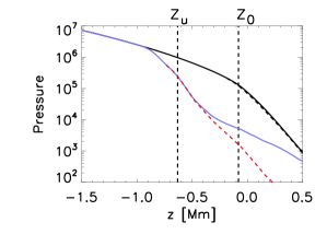
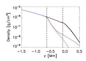
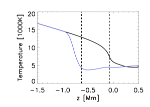
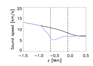
Figure 1.: The red-dashed curves show the semi-empirical umbral model from Maltby et al. (1986) as a function of height. The black curves are the quiet-Sun values from model-S. The blue curves show the pressure the umbral model described in this paper. The panels show: presssure (top-left panel), density (top-right), temperature (bottom-left), and sound-speed (bottom-right). The vertical dashed lines are the heights where $\tau_{5000}=1$ in the quiet-Sun ($z=z_{0}$) and the umbra ($z=z_{\rm u}$).fig˙atm˙umbra

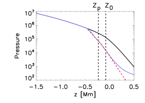
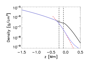
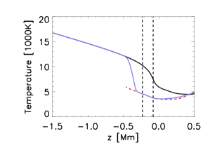
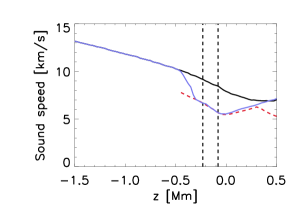
Figure 2.: The red-dashed curves show the semi-empirical penumbral model from Ding and Fang (1989). The black curves are the quiet-Sun values from Model S. The blue curves show the penumbral model described in this paper. Shown are, the pressure (top-left panel), density (top-right), temperature (bottom-left), and sound-speed (bottom-right). The vertical dashed lines are the heights where $\tau_{5000}=1$ in the quiet-Sun ($z=z_{0}$) and the penumbra ($z=z_{\rm p}$).fig˙atm˙penumbra

2.2 Geometrical aspects

The umbral and penumbral models discussed above need to be smoothly embedded in Model S. In order to do so, we modify the semi-empirical models above and below the $\tau_{5000}=1$ levels of the umbra and the penumbra, as follows.

In our model, the pressure along the axis of the sunspot, denoted by $P_{\rm u}$, is such that

$$\ln P_{\rm u}(z)=w(z)\ln P_{\mathrm{Maltby}}(z)+(1-w(z))\ln P_{\mathrm{qs}}(z).$$ (3)

In this expression, $P_{\mathrm{Maltby}}(z)$ is the umbral pressure given by Maltby et al. (1986) for $z>-736$ km, and is extrapolated for $z<-736$ km assuming constant pressure scale height. The quantity $P_{\mathrm{qs}}(z)$ is the quiet-Sun pressure from Model S. The function $w(z)$ is a weighting function given by

$$w(z)=\left\{\begin{array}[]{l l}0&z\leq z_{\rm{u}}-380\;\mbox{km},\\ \cos[\pi\frac{(z_{\rm{u}}-80\;\mbox{km}-z)}{300\;\mbox{km}}]/2+1/2&z_{\rm{u}}-380\;\mbox{km}<z\leq z_{\rm{u}}-80\;\mbox{km},\\ 1&z_{\rm{u}}-80\;\mbox{km}<z\leq z_{\rm{u}}+20\;\mbox{km},\\ \cos[\pi\frac{(z_{\rm{u}}+20\;\mbox{km}-z)}{(900\;\mbox{km}-z_{\rm{u}})}]/2+1/2&z_{\rm{u}}+20\;\mbox{km}<z\leq 900\;\mbox{km},\\ 0&900\;\mbox{km}<z.\end{array}\right.$$ (4)

The resulting umbral pressure is plotted in Figure fig_atm_umbra. The pressure near $z=z_{\rm u}$ is that of Maltby et al. (1986). Below, it smoothly merges with the quiet Sun pressure at $z=z_{\rm u}-380\;\rm{km}=-1000$ km. Above, the pressure tends to the quiet-Sun value and there is a significant departure from Maltby et al. (1986) for $z\gtrsim-200$ km (by more than a factor of two).

The vertical profile of the density is treated in the same manner as the pressure. The Maltby model does not explicitly contain all the properties that we require, so we use the OPAL tables to derive the sound speed from the pressure and the density.

The penumbral pressure and the density of Ding and Fang (1989) are embedded in Model S in a similar way as was done for the umbra, except that the weighting function $w(z)$ is replaced by

$$w(z)=\left\{\begin{array}[]{l l}0&z\leq z_{\rm{p}}-280\;\mbox{km},\\ \cos[\pi\frac{(z_{\rm{p}}-80\;\mbox{km}-z)}{200\;\mbox{km}}]/2+1/2&z_{\rm{p}}-280\;\mbox{km}<z\leq z_{\rm{p}}-80\;\mbox{km},\\ 1&z_{\rm{p}}-80\;\mbox{km}<z\leq z_{\rm{p}}+20\;\mbox{km},\\ \cos[\pi\frac{(z_{\rm{p}}+20\;\mbox{km}-z)}{(800\;\mbox{km}-z_{\rm{p}})}]/2+1/2&z_{\rm{p}}+20\;\mbox{km}<z\leq 800\;\mbox{km}\\ 0&800\;\mbox{km}<z.\end{array}\right.$$ (5)

The resulting penumbral pressure and density are plotted in Figure fig_atm_penumbra.

Thus far we have described umbral, penumbral, and quiet-Sun models. We use them to form a three-dimensional cylindrically-symmetric sunspot model.

Since we are modeling only the very near-surface layers of the sunspot (top  1 Mm), we do not pay excessive attention to the fanning of the interfaces with depth. In our 3D sunspot model, each thermodynamic quantity is the product of a function of $z$ and a function of $r$.

The radii of the umbra and the penumbra are denoted by $r_{\rm u}$ and $r_{\rm p}$. We combine the three model components (umbra, penumbra, quiet-Sun) in the $r$ coordinate using the weight functions shown in Figure fig_weights. The transitions between the 1-D atmospheres have a width of $6$ Mm and are described by raised cosines.

For the sunspot in Active Region 9787, we take $r_{\rm{u}}=10$ Mm and $r_{\rm{p}}=20$ Mm for the umbral and penumbral radii.

The sound speed was again reconstructed using the density, pressure, and the OPAL tables to ensure consistency. We note that the temperature does not appear in the equations and is used only for the purpose of calculating the properties of the spectral lines used in helioseismology (e.g., the MDI Ni 676.8 nm line).

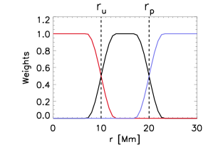
Figure 3.: Relative weights used to combine the umbral (red), penumbral (black), and quiet-Sun (blue) models in the horizontal radial direction.fig˙weights

2.3 Observables

Doppler velocity is the primary observable in helioseismology. In this section, which is parenthetical, we consider the question of how to compute a quantity resembling the observations from the sunspot model. This topic has previously been considered by, e.g., Wachter (2008). Here we use the STOPRO code (Solanki, 1987) to synthesize, assuming LTE, the formation of the Ni 676.8 nm line, which is the line used by the SOHO/MDI instrument.

We obtain a continuum intensity image near the Ni line, shown in Figure fig_sim_I, together with observations. The bright rings at the transitions between the umbra, penumbra, and quiet Sun are undesirable artifacts due to the simplified transitions between the different model components. This may have to be addressed in a future study by adjusting the weights from Figure fig_weights.

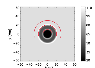
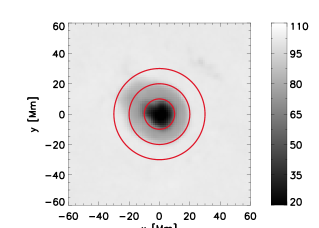
Figure 4.: Left panel: Model of the sunspot continuum intensity image near the Ni $676.8$ nm line calculated using STOPRO. The red arcs have radii 10 Mm, 20 Mm, and 30 Mm. Noticeable are bright rings at the transitions between the umbra, penumbra, and quiet Sun. Right panel: Observed SOHO/MDI intensity image of the sunspot in AR 9787 averaged over 20 – 28 January 2002. fig˙sim˙I

We compute the response functions for vertical velocity perturbations (Beckers and Milkey, 1975) as functions of height, horizontal position, and wavelength, $\lambda$. We integrate the response function over the wavelength bandpass [$-100$ mÅ, $-34$ mÅ] measured from line center. This wavelength range was chosen because it is where the slope of the line is maximal, i.e. where the response to velocity perturbations is largest. The response function is normalized so that its $z$-integral is unity at each horizontal position. These are the weights (Figure fig_sim_rf) to be multiplied by the vertical velocity and then integrated in the vertical direction to give a Doppler velocity map.

Whether the bright rings affect the Doppler velocity in practice is unclear. We believe, however, that the response function computed here will be useful in studies investigating the diagnostic potential of the helioseismic signal within the sunspot.

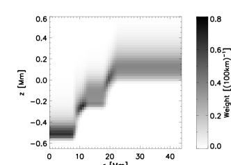
Figure 5.: The weights (being the normalized response function of the Ni 676.8 nm line) which allow us to create synthetic helioseismic Doppler velocity maps. The height is with reference to the $\tau_{5000}=1$ surface in the quiet-Sun. fig˙sim˙rf

2.4 Magnetic field

When observations of the vector magnetic field are available, they can and should be included in constraining the sunspot model. In this paper, we consider a more generic case and assume a Gaussian dependence of the vertical magnetic field in the radial direction. The important parameters are then the maximum magnetic field at the surface, $B_{0}$, the half-width at half maximum (HWHM) of the Gaussian profile at the surface, $h_{0}$, and the inclination of the magnetic field at the umbral-penumbral boundary.

Explicitly, the dependence of $B_{z}$ on $r$ and $z$ is given by

$$B_{z}(r,z)=B_{z}(r=0,z)\exp[-(\ln 2)r^{2}/h(z)^{2}]$$ (6)

where $h(z)$ is the half width at half maximum (HWHM) of the Gaussian. Since the magnetic flux at each height must be conserved, we have

$$h(z)=h_{0}\sqrt{B_{0}/B_{z}(r=0,z)},$$ (7)

where $h_{0}$ is the surface value of $h$. For the sunspot in Active Region 9787 we have chosen $B_{0}=3$ kG and $h_{0}=10$ Mm.

The function $B_{z}(r=0,z)$ is unknown. It is a goal of helioseismology to constrain $B_{z}$ along the sunspot axis. Here we choose a two-parameter function as follows:

$$B_{z}(r=0,z)=B_{0}e^{-(z/\alpha)L(-z/\alpha)L(z/\alpha_{2})},$$ (8)

where $L(z)=1/(1+e^{-z})$ is the logistic function. Since $dB_{z}/dz(r=0,z=0)=-B_{0}/(4\alpha)$, the parameter $\alpha$ controls the vertical gradient of $B_{z}$ near the surface. Together with the condition $\nabla\cdot{\bf B}=0$, $dB_{z}/dz(r=0,z=0)$ determines the full surface vector magnetic field. We chose $\alpha=1.25$ Mm so that at $z=0$ the inclination of the magnetic field is $45^{\circ}$ at the umbra/penumbra boundary, in agreement with observations. The parameter $\alpha_{2}$ controls the field strength at depth; we chose $\alpha_{2}=18.4$ Mm.

Figure fig_spot_field summarizes the magnetic properties of the sunspot model. The magnetic field strength increases rapidly with depth as a consequence of the choice of a large $\alpha_{2}$ in Equation (eq.logistic). Equation (eq.radspot) implies in turn that the radius of the tube shrinks fast, from 10 Mm at the surface down to $1.3$ Mm at $z=-25$ Mm (just spatially resolved in the numerical simulations of Section 3). This sunspot model—as monolithic as imaginable—is only one possible choice among many. We note that it would be straightforward to consider model sunspots that fan out as a function of depth, e.g., by decreasing the parameter $\alpha_{2}$. Figure fig_spot_field also shows the ratio of the fast-mode speed, $v_{\rm f}$, to the sound speed, $c$, along the sunspot axis, which is nearly unity for depths greater than 1 Mm, but increases very rapidly near the surface. For example, we have $v_{\rm f}/c=1.9$ at $z=z_{u}$ and $v_{\rm f}/c=3.9$ at $z=-400$ km. The height at which the Alfvén and sound speeds are equal ($a=c$) is $z=-750$ km.

We comment that the construction of both the thermodynamic and magnetic properties of this model aims to get the surface properties correct. Additional information about the surface, when available, could easily be incorporated into our sunspot model. Where information is missing the assumption that the sunspot has similar properties to those of other sunspots is possibly the best that can be done. A summary of the choices made to model the sunspot in AR 9787, which was observed by MDI, is given in Table 1.

Figure 6.: The upper left panel shows the vertical magnetic field strength along the axis of the spot. The upper right panel shows the ratio of the fast mode speed to the sound speed also along the sunspot axis. The lower panels show the inclination (left) and strength (right) of the magnetic field at $z=0$ fig˙spot˙field

Table 1.: Basic choices made in constructing the sunspot model for AR 9787.

Umbral model	Maltby et al. (1986)
Penumbral model	Ding and Fang (1989)
Umbral radius	$r_{\rm{u}}=10$ Mm
Penumbral radius	$r_{\rm{p}}=20$ Mm
Umbral depression ($\tau_{5000}=1$)	$z_{0}-z_{\rm{u}}$ = 550 km
Penumbral depression ($\tau_{5000}=1$)	$z_{0}-z_{\rm{p}}$ = 150 km
On-axis surface vertical field	$B_{0}$ = 3 kG
Radial profile of $B_{z}$	Gaussian with HWHM=10 Mm
Field inclination at umbra/penumbra boundary	$45^{\circ}$

3 Numerical simulation of the propagation of waves through the sunspot model

We want to simulate the propagation of planar wave packets through the model sunspot and surrounding quite-Sun using the SLiM code described in Cameron, Gizon, and Daiffallah (2007) and Cameron, Gizon, and Duvall (2008). The size of the box is $145.77$ Mm in both horizontal coordinates. We used 200 Fourier modes in each of the two horizontal directions; almost all of the wave energy resides in the 35 longest horizontal wavelengths. The vertical extent of the box is $-25$ Mm $<z<2.5$ Mm, where the physical domain, $-20$ Mm $<z<0.5$ Mm, is sandwiched between two ”sponge” layers that reduce strongly wave reflection from the boundaries (Cameron, Gizon, and Duvall, 2008). We use 1098 grid points and a finite difference scheme in the vertical direction.

Thus far the quiet-Sun reference model has been Model S which is convectively unstable. For the purpose of computing the propagation of solar waves through our sunspot models using linear numerical simulations, we need a stable background model in which to embed the sunspot model. We use Convectively Stabilized Model B (CSM_B) from Schunker et al. (2010). We keep the relative perturbations in pressure, density, and sound speed fixed. For example, this means that the new pressure is given by

$$p(r,z)=P(r,z)\;\frac{P_{\mathrm{CSM\_B}}(z)}{P_{\mathrm{qs}}(z)},$$ (9)

where $P(r,z)$ is the pressure as discussed above. The same treatment is applied to density, $\rho$, and sound speed, $c$.

Separate simulations are done for f, p₁, and p₂ wave packets. In each case, a wave packet is made of approximately 30 Fourier modes. At $t=0$ all the modes are in phase at $x=-43.73$ Mm, while the sunspot is centered at $x=y=0$. The initial conditions at $t=0$ are such that the wave packet propagates in the positive $x$ direction, towards the sunspot.

The Alfvén velocity increases strongly above the photospheric layers of the spot (see Figure fig_spot_field). This is a problem for two reasons. The first and most important of these is that it causes the wavelengths of both the fast-mode and Alfvén waves to become very large. The upper boundary, which is located at $z=2.5$ Mm, becomes only a fraction of a wavelength away from the surface. This makes the simulation sensitive to the artificial upper boundary. The second reason is that our code is explicit and hence subject to a CFL condition: High wave speeds require very small time steps and correspondingly large amounts of computer power. In order to address this problem, we notice that we expect all solar waves that reach the region where the Alfvén speed is high to continue to propagate upward out of the domain. We therefore reduce the Alfvén speed in this region in the simulation to increase the time the waves spend in the sponge layer. This reduces the influence of the upper boundary and allows us to have a larger time step. In practice, we multiply the Lorentz force by $8c^{2}/(8c^{2}+a^{2})$, where $a(r,z)$ is the Alfvén speed, and $c(z)$ is the sound speed of the quiet Sun at the same height. This limits the fast-mode speed to be a maximum of three times the quiet-Sun sound speed at the same geometric height. Since the sound speed near the $\tau=1$ layer in the spot is less than half of that of the quiet Sun at the same height, the maximum value of the fast mode speed in this critical region is approximately six times the local sound speed. The functional form chosen to limit the Lorentz force modifies $a$ at and below the $c=a$ level by less than 2%. This corresponds to a change in field strength of less than 30 G or a minimal change in the height of the $c=a$ surface.

4 Preliminary comparison of simulations with observed MDI cross-covariances of the Doppler velocity

There exist excellent observations (SOHO/MDI Doppler velocity) of helioseismic waves around the sunspot in AR 9787 (Gizon et al., 2009). The wave field around the sunspot can be characterized by the temporal cross-covariance of the observed random wave field. It has been argued (Gizon, Birch, and Spruit, 2010, and references therein) that the observed cross-covariance is closely related to the Green’s function (the response of the Sun to a localized source). Hence the observed cross-covariance is comparable to the surface vertical velocity from initial-value numerical simulations of the wave packet propagation. In Cameron, Gizon, and Duvall (2008) we studied the propagation of an f-mode wave packet through a simplified magnetohydrostatic sunspot model. We found that we could constrain the surface magnetic field by comparing the observed f-mode cross-covariance with a simulated f-mode wave packet.

Here we assess the seismic signature of the semi-empirical sunspot model described in Section 2 by comparing the simulations and observations. The cross-covariance is constructed in the same way as in Cameron, Gizon, and Duvall (2008), to which we refer the reader. In short, it is computed according to

$$C(x,y,t)=\int_{0}^{T}{\bar{\phi}}(t^{\prime})\phi(x,y,t^{\prime}+t)\,dt^{\prime},$$ (10)

where $T=7$ days is the observation time, $\phi$ is the observed Doppler velocity, ${\bar{\phi}}$ is the average of $\phi$ over the line $x=-43.73$ Mm, and $t$ is the time lag. We select three different wave packets (f, p₁, and p₂) by filtering $\phi$ along particular mode ridges. As said in Section 3, for the numerical simulations we consider plane wave packets starting at $x=-43.73$ Mm and propagating in the $+x$ direction towards the model sunspot (at the origin). The initial conditions of the simulation are chosen such that, in the far field, the simulated vertical velocity has the same temporal power as the observed cross-covariance.

Figure fig_p1_s shows the observed cross-covariances and simulated wave packets for the p₁ modes at four consecutive time lags. The main features seen in the cross-covariances, the speedup of the waves across the sunspot as well as their loss of energy at short wavelengths, are also seen in the simulations. The details of the perturbed waveforms can only be understood in the context of finite-wavelength scattering (Gizon, Hanasoge, and Birch, 2006).

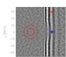
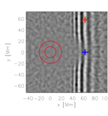
Figure 7.: (Left panels) Simulated vertical velocity of p₁ wave packets at times $t=0,$ 140, 144, and 148 min (from top to bottom). White shades are for positive values, dark shades for negative values. The gray scale covers the full range of values in each row. (Right panels) Observed cross-covariance at the corresponding time-lags. The $t=0$ frame from the simulation is the prescribed initial condition. The red and blue crosses (hereafter points A and B respectively) indicate two particular locations used in the subsequent analysis (Figures fig_ts and fig_fd).fig˙p1˙s

For a more detailed comparison we have concentrated on the two spatial locations $A=(x,y)=(60,0)$ Mm and $B=(60,60)$ Mm, marked with crosses in Figure fig_p1_s. The first point lies behind the sunspot, where the effects of the sunspot are easily noticeable. The second point is away from the scattered field and serves as a quiet-Sun reference. The corresponding simulated and observed wave packets are plotted as functions of time in Figure fig_ts. The match again looks qualitatively good.

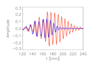
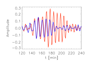
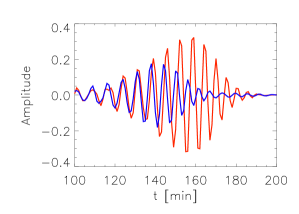
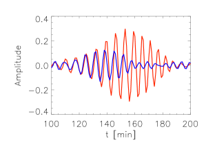
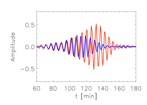
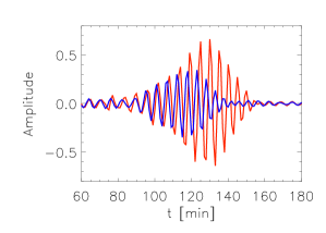
Figure 8.: Time series from the simulations (left panels) or from the observed cross-covariance (right panels) for the (top to bottom) f, p₁ and p₂ wave packets. The red curve corresponds to point A (the red cross) in Figure fig_p1_s, the blue curve to point B (the blue cross).fig˙ts

To proceed further we Fourier analyze the time series at points A and B: we consider the power spectra and phases. The temporal power spectra are shown in the left panels of Figure fig_fd. The power spectrum of the simulations is similar to that of cross-covariance for the p₁ modes, less so for the f and p₂ modes. We note that the differences between the simulated and observed power spectra are seen at both spatial points. We also analyzed the phase difference between the wave packets at the two points (A minus B) as a function of frequency (Figure fig_fd). The phase shifts introduced by the sunspot are reasonably well reproduced by the simulations, although some differences exist especially for the f modes.

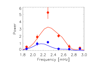
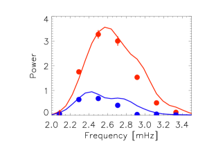
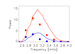
Figure 9.: Frequency analysis of the curves shown in Figure 8. The left panels shows the power spectra of the time series from Figure 8, with the solid lines indicating the values for the numerical simulations and the dots indicating the values from the observed cross-covariances. The red curves are for point B (away from the sunspot) abd the blue curves for point A (behind the sunspot). The top panels are for f mode wave packets, the middle for p₁, and the bottom for p₂. The right panels show the phase differences between points A and B, i.e. sunspot minus quiet-Sun. The solid lines are for the numerical simulations and the dots are for the observations. The error bars are root-mean-square deviations computed over $0.3$-mHz intervals. fig˙fd

In both the observations and the simulations we see that the power in the f and p₁ wavepackets peaks substantially below $3$ mHz. The reason for this can be understood by noting that wave attenuation increases sharply with frequency. Even though the initial power spectra have most of their energy near 3 mHz, very little of the power at and above 3 mHz reaches the points $A$ and $B$. The remaining low frequency waves have more sensitivity to the deeper layers and are thus the most important in determining the subsurface structure of the sunspot. It is also apparent that the sunspot more strongly ’damps’ higher frequency waves. This is understandable since these waves have more of their energy in the near-surface region, where mode conversion (from the f and p modes into Alfvén and slow-magnetoacoustic modes that propagate away from the surface) is efficient. Over the frequency range studied, the power ’absorption’ coefficient increases with frequency (in accordance with Braun, 1995; Braun and Birch, 2008). The same trend is also seen in the phase shifts, with low frequency waves being almost unaffected by the sunspot whilst high frequency waves have phase shifts which range up to 300 degrees (for the frequencies shown). A strong frequency dependence of the travel-time perturbations had already been reported by Braun and Birch (2008) for ridges p₁ through p₄ (see also Braun and Birch, 2006; Birch et al., 2009). The reason why the phase shifts are strongest for high-frequency waves is again that they have more energy near the surface. The possibility of such strong phase shifts should be born in mind when interpreting (and measuring) helioseismic waves near sunspots.

5 Conclusion

We have outlined a method for constructing magnetic models of the near-surface layers of sunspots by including available observational constraints and semi-empirical models of the umbra and penumbra. Applying this type of model to the sunspot of AR 9787, we showed that the observed helioseismic signature of the sunspot model is reasonably well captured. Our approach was to compare numerical simulations of wave propagation through the model sunspot and the observed SOHO/MDI cross-covariances of the Doppler velocity.

Possible improvements of the simulation include a better treatment of wave attenuation (esp. in plage), improved initial conditions, and inclusion of the moat flow. It should also be noted that improved observations of the surface vector magnetic field by SDO/HMI will help tune the sunspot models.

The dominant influence of the sunspot’s surface layers on helioseismic waves means that it is necessary to model it very well in order to extract information from the much weaker signature of the sunspot’s subsurface structure. The sunspot model used here accounts for most of the helioseismic signal, although there are substantial differences that remain to be explored. In any case, the model provides a testbed which is sufficiently similar to a real sunspot to be used for numerous future studies in sunspot seismology.

Finally, we remark that our numerical simulations of linear waves could potentially be used to interpret other helioseismic observations than the cross-covariance (cf. helioseismic holography or Fourier-Hankel analysis), as well as other magnetic phenomena (e.g., small magnetic flux tubes, see Duvall, Birch, and Gizon, 2006).

References

- Beckers and Milkey (1975) Beckers, J.M., Milkey, R.W.: 1975, The line response function of stellar atmospheres and the effective depth of line formation. Sol. Phys. 43, 289 – 292. doi:10.1007/BF00152353.
- Birch et al. (2009) Birch, A.C., Braun, D.C., Hanasoge, S.M., Cameron, R.: 2009, Surface-Focused Seismic Holography of Sunspots: II. Expectations from Numerical Simulations Using Sound-Speed Perturbations. Sol. Phys. 254, 17 – 27. doi:10.1007/s11207-008-9282-9.
- Braun (1995) Braun, D.C.: 1995, Scattering of p-Modes by Sunspots. I. Observations. ApJ 451, 859. doi:10.1086/176272.
- Braun and Birch (2006) Braun, D.C., Birch, A.C.: 2006, Observed Frequency Variations of Solar p-Mode Travel Times as Evidence for Surface Effects in Sunspot Seismology. ApJ 647, L187 – L190. doi:10.1086/507450.
- Braun and Birch (2008) Braun, D.C., Birch, A.C.: 2008, Surface-Focused Seismic Holography of Sunspots: I. Observations. Sol. Phys. 251, 267 – 289. doi:10.1007/s11207-008-9152-5.
- Cameron, Gizon, and Daiffallah (2007) Cameron, R., Gizon, L., Daiffallah, K.: 2007, SLiM: a code for the simulation of wave propagation through an inhomogeneous, magnetised solar atmosphere. Astronomische Nachrichten 328, 313. doi:10.1002/asna.200610736.
- Cameron, Gizon, and Duvall (2008) Cameron, R., Gizon, L., Duvall, T.L. Jr.: 2008, Helioseismology of Sunspots: Confronting Observations with Three-Dimensional MHD Simulations of Wave Propagation. Sol. Phys. 251, 291 – 308.
- Christensen-Dalsgaard et al. (1996) Christensen-Dalsgaard, J., Dappen, W., Ajukov, S.V., Anderson, E.R., Antia, H.M., Basu, S., Baturin, V.A., Berthomieu, G., Chaboyer, B., Chitre, S.M., Cox, A.N., Demarque, P., Donatowicz, J., Dziembowski, W.A., Gabriel, M., Gough, D.O., Guenther, D.B., Guzik, J.A., Harvey, J.W., Hill, F., Houdek, G., Iglesias, C.A., Kosovichev, A.G., Leibacher, J.W., Morel, P., Proffitt, C.R., Provost, J., Reiter, J., Rhodes, E.J. Jr., Rogers, F.J., Roxburgh, I.W., Thompson, M.J., Ulrich, R.K.: 1996, The Current State of Solar Modeling. Science 272, 1286. doi:10.1126/science.272.5266.1286.
- Ding and Fang (1989) Ding, M.D., Fang, C.: 1989, A semi-empirical model of sunspot penumbra. A&A 225, 204 – 212.
- Duvall, Birch, and Gizon (2006) Duvall, T.L. Jr., Birch, A.C., Gizon, L.: 2006, Direct Measurement of Travel-Time Kernels for Helioseismology. ApJ 646, 553 – 559. doi:10.1086/504792.
- Gizon, Birch, and Spruit (2010) Gizon, L., Birch, A.C., Spruit, H.C.: 2010, Local Helioseismology: Three Dimensional Imaging of the Solar Interior. Ann. Rev. Astron. Astrophys. 48, accepted. ArXiv:1001.0930.
- Gizon, Hanasoge, and Birch (2006) Gizon, L., Hanasoge, S.M., Birch, A.C.: 2006, Scattering of Acoustic Waves by a Magnetic Cylinder: Accuracy of the Born Approximation. ApJ 643, 549 – 555. doi:10.1086/502623.
- Gizon et al. (2009) Gizon, L., Schunker, H., Baldner, C.S., Basu, S., Birch, A.C., Bogart, R.S., Braun, D.C., Cameron, R., Duvall, T.L., Hanasoge, S.M., Jackiewicz, J., Roth, M., Stahn, T., Thompson, M.J., Zharkov, S.: 2009, Helioseismology of Sunspots: A Case Study of NOAA Region 9787. Space Science Reviews 144, 249 – 273. doi:10.1007/s11214-008-9466-5.
- Hanasoge (2008) Hanasoge, S.M.: 2008, Seismic Halos around Active Regions: A Magnetohydrodynamic Theory. ApJ 680, 1457 – 1466. doi:10.1086/587934.
- Khomenko and Collados (2008) Khomenko, E., Collados, M.: 2008, Magnetohydrostatic Sunspot Models from Deep Subphotospheric to Chromospheric Layers. ApJ 689, 1379 – 1387. doi:10.1086/592681.
- Khomenko, Collados, and Felipe (2008) Khomenko, E., Collados, M., Felipe, T.: 2008, Nonlinear Numerical Simulations of Magneto-Acoustic Wave Propagation in Small-Scale Flux Tubes. Sol. Phys. 251, 589 – 611. doi:10.1007/s11207-008-9133-8.
- Maltby et al. (1986) Maltby, P., Avrett, E.H., Carlsson, M., Kjeldseth-Moe, O., Kurucz, R.L., Loeser, R.: 1986, A new sunspot umbral model and its variation with the solar cycle. ApJ 306, 284 – 303. doi:10.1086/164342.
- Mathew et al. (2003) Mathew, S.K., Lagg, A., Solanki, S.K., Collados, M., Borrero, J.M., Berdyugina, S., Krupp, N., Woch, J., Frutiger, C.: 2003, Three dimensional structure of a regular sunspot from the inversion of IR Stokes profiles. A&A 410, 695 – 710. doi:10.1051/0004-6361:20031282.
- Mathew et al. (2004) Mathew, S.K., Solanki, S.K., Lagg, A., Collados, M., Borrero, J.M., Berdyugina, S.: 2004, Thermal-magnetic relation in a sunspot and a map of its Wilson depression. A&A 422, 693 – 701. doi:10.1051/0004-6361:20040136.
- Moradi and Cally (2008) Moradi, H., Cally, P.S.: 2008, Time-Distance Modelling in a Simulated Sunspot Atmosphere. Sol. Phys. 251, 309 – 327. doi:10.1007/s11207-008-9190-z.
- Moradi, Hanasoge, and Cally (2009) Moradi, H., Hanasoge, S.M., Cally, P.S.: 2009, Numerical Models of Travel-Time Inhomogeneities in Sunspots. ApJ 690, L72 – L75. doi:10.1088/0004-637X/690/1/L72.
- Moradi et al. (2009) Moradi, H., Baldner, C., Birch, A., Braun, D., Cameron, R., Duvall Jr., T., Gizon, L., Haber, D., Hanasoge, S., Jackiewicz, J., Khomenko, E., Komm, R., Rajaguru, R., Rempel, M., Roth, M., Schlichenmaier, R., Schunker, H., Spruit, H., Strassmeier, K., Thompson, M., Zharkov, S.: 2009, Modeling the subsurface structure of sunspots. Sol. Phys., submitted.
- Parchevsky and Kosovichev (2009) Parchevsky, K.V., Kosovichev, A.G.: 2009, Numerical Simulation of Excitation and Propagation of Helioseismic MHD Waves: Effects of Inclined Magnetic Field. ApJ 694, 573 – 581. doi:10.1088/0004-637X/694/1/573.
- Schunker et al. (2010) Schunker, H., Cameron, R., Gizon, L., Moradi, H.: 2010, Convectively stabilised background solar models for numerical local helioseismology. Sol. Phys., in preparation.
- Solanki (1987) Solanki, S.K.: 1987, Thesis no. 8309. PhD thesis, Institut für Astronomie, ETH Zentrum, Zürich, Switzerland.
- Solanki (2003) Solanki, S.K.: 2003, Sunspots: An overview. A&A Rev. 11, 153 – 286. doi:10.1007/s00159-003-0018-4.
- Thomas and Weiss (2008) Thomas, J.H., Weiss, N.O.: 2008, Sunspots and Starspots, Cambridge University Press, Cambridge, UK.
- Wachter (2008) Wachter, R.: 2008, Instrumental Response Function for Filtergraph Instruments. Sol. Phys. 251, 491 – 500. doi:10.1007/s11207-008-9197-5.