Hybrid functionals within the all-electron FLAPW method:
implementation and applications of PBE0

Abstract

We present an efficient implementation of the Perdew-Burke-Ernzerhof hybrid functional PBE0 within the full-potential linearized augmented-plane-wave (FLAPW) method. The Hartree-Fock exchange term, which is a central ingredient of hybrid functionals, gives rise to a computationally expensive nonlocal potential in the one-particle Schrödinger equation. The matrix elements of this exchange potential are calculated with the help of an auxiliary basis that is constructed from products of FLAPW basis functions. By representing the Coulomb interaction in this basis the nonlocal exchange term becomes a Brillouin-zone sum over vector-matrix-vector products. The Coulomb matrix is calculated only once at the beginning of a self-consistent-field cycle. We show that it can be made sparse by a suitable unitary transformation of the auxiliary basis, which accelerates the computation of the vector-matrix-vector products considerably. Additionally, we exploit spatial and time-reversal symmetry to identify the nonvanishing exchange matrix elements in advance and to restrict the $\mathbf{k}$ summations for the nonlocal potential to an irreducible set of $\mathbf{k}$ points. Favorable convergence of the self-consistent-field cycle is achieved by a nested density-only and density-matrix iteration scheme. We discuss the convergence with respect to the parameters of our numerical scheme and show results for a variety of semiconductors and insulators, including the oxides $\mathrm{ZnO}$, $\mathrm{EuO}$, $\mathrm{Al_{2}O_{3}}$, and $\mathrm{SrTiO_{3}}$, where the $\mathrm{PBE0}$ hybrid functional improves the band gaps and the description of localized states in comparison with the PBE functional. Furthermore, we find that in contrast to conventional local exchange-correlation functionals ferromagnetic $\mathrm{EuO}$ is correctly predicted to be a semiconductor.

I Introduction

Within the last decades density-functional theory (DFT) (Refs. Hohenberg-Kohn, and DFT-review, ) has evolved into the state of the art of electronic-structure calculations. It is usually applied within the Kohn-Sham (KS) formalism,(Kohn-Sham, ) which maps the interacting many-electron system onto a noninteracting system with the same density. All exchange and correlations effects of the many-electron system are incorporated into the so-called exchange-correlation (xc) energy functional, which is not known exactly and must be approximated in practice. The choice of the xc functional is the only practical approximation in this otherwise exact theory and determines the precision and efficiency of the numerical DFT calculations.

Fortunately, already the local-density approximation (LDA),(Ceperley_and_Adler, ; VWN, ) where the xc energy functional is approximated locally by that of the homogeneous electron gas, gives reliable results for a wide range of materials and properties. The generalized gradient approximation (GGA) (Refs. Generalized_Gradient_Approximation_Made_Simple, and Accurate_and_simple_density_functional_for_the_electronic_exchange_energy:_Generalized_gradient_approximation, ) goes beyond this approximation by incorporating also the density gradient of the inhomogeneous system. Due to its improved accuracy the GGA has led to many applications of DFT in quantum chemistry. However, there are still many cases where LDA and GGA give poor results or are even qualitatively wrong. Among these cases are the band gaps of solids, the atomization energies, bond lengths, and adsorption sites of molecules as well as systems with localized states such as transition-metal oxides. During the last decade hybrid functionals, which combine a local or semilocal xc functional with nonlocal Hartree-Fock (HF) exchange, have been shown to overcome these deficiencies to a great extent.(Density-functional_thermochemistry_III(Becke), ; Toward_reliable_density_functional_methods_without_adjustable_parameters:_The_pbe0_model, ; On_the_prediction_of_band_gaps_from_hybrid_functional_theory, ; MnO, ; MgO-NiO-CoO, ) Hybrid functionals are usually applied within the generalized Kohn-Sham (gKS) scheme,(Generalized_Kohn-Sham_schemes_and_the_band_gap_problem, ) where the HF exchange term leads to a nonlocal exchange potential in the one-particle equations. The first hybrid functional, a half-and-half mixing of the LDA functional with HF exchange, was proposed by Becke in 1993.(Half-and-half-mixing, ) Since then various ab initio and semiempirical hybrid functionals have been published.(Rationale_for_mixing_exact_exchange_with_density_functional_approximations, ; Density-functional_thermochemistry_III(Becke), ; B3LYP, ; TPSSh, ) The PBE0 functional,Rationale_for_mixing_exact_exchange_with_density_functional_approximations on which we focus in this paper, does not contain any empirical parameters and is thus an ab initio hybrid functional.

Hybrid functionals for systems with periodic boundary conditions were first implemented in the late 1990s within a basis of Gaussian-type functions and the pseudopotential plane-wave approach.(Crystall98, ; PP-PW, ) In 2005 Paier et al.(PAW-hybrid, ) developed an implementation within the projector-augmented-wave (PAW) technique. In 2006 Novak et al.(Exact_exchange_for_correlated_electrons, ) proposed an approximate scheme within the full-potential linearized augmented-plane-wave (FLAPW) approach. There the nonlocal exchange term is evaluated only in individual atomic spheres and only for selected $l$ channels. In this paper, we present an efficient numerical implementation of hybrid functionals within the FLAPW method, which does not suffer from these constraints. The FLAPW method provides a highly accurate basis for all-electron calculations, with which a large variety of materials, including open systems with low symmetry, $d$- and $f$-electron systems as well as oxides, can be studied. It treats core and valence electrons on an equal footing.

In the first Hartree-Fock implementation within the FLAPW method, Massidda et al.(Hartree-Fock_LAPW_approach_to_the_electronic_properties_of_periodic_systems, ) employed an algorithm that is routinely used to generate the potential created by the electronic and nuclear charges and thus solves the Poisson equation.(Solution_of_poissons_equation, ) This Poisson solver can also be used for the nonlocal exchange potential because its matrix representation involves formally identical six-dimensional integrals over space. Instead of the real charge one then uses an artificial charge formed by the product of two wave functions. Unfortunately, although the algorithm is very fast, the Poisson solver must be called many times instead of just once when applied to the exchange potential, which makes this approach computationally very expensive.

In this paper we propose an alternative approach that employs an auxiliary basis, the so-called mixed product basis, which is constructed from products of LAPW basis functions and consists of muffin-tin (MT) functions and interstitial plane waves.(All_electron_GW_approximation_with_the_mixed_basis_expansion_based_on_the_full_potential_LMTO_method, ) This basis allows to decompose the state-dependent six-dimensional integral into two three-dimensional and one state-independent six-dimensional integral, which is the Coulomb matrix represented in the mixed product basis. The Coulomb matrix is calculated once at the beginning of the self-consistent-field cycle while only the three-dimensional integrals must be evaluated in each iteration. In this formulation the matrix elements of the nonlocal exchange potential are evaluated as Brillouin-zone (BZ) sums over vector-matrix-vector products. Furthermore, by a suitable unitary transformation, nearly all MT functions become multipole-free, which makes the Coulomb matrix sparse and reduces the computational effort for the vector-matrix-vector products considerably. As the exchange interaction is small compared with the other energy terms, we introduce a band cutoff as a convergence parameter and construct the exchange matrix only in the reduced Hilbert space formed by the wave functions up to this cutoff. In this way the number of matrix elements that must be calculated explicitly is reduced. Because of spatial and time-reversal symmetry some of the exchange matrix elements vanish. In order to decide in advance, which of the matrix elements will be nonzero, we employ a simple auxiliary operator, which has the same symmetry properties as the nonlocal exchange potential. Additionally, we use group theory to restrict the $\mathbf{k}$ summations for the nonlocal exchange term to the smaller set of $\mathbf{k}$ points, which are inequivalent with respect to the group of symmetry operations.

The long-range nature of the Coulomb interaction gives rise to a divergence of the Coulomb matrix in the center of the BZ leading to a divergent integrand in the exchange matrix elements. In a previous publication we showed that the Coulomb matrix in the mixed product basis can be decomposed exactly into a divergent and a nondivergent part.(Friedrich, ) The resulting divergent integrand is then given analytically and can be integrated exactly while the nondivergent part is treated with standard numerical integration techniques. We also calculate corrections beyond the divergent $1/q^{2}$ term, which are obtained from $\mathbf{k}\cdot\mathbf{p}$ perturbation theory.

The paper is organized as follows. Section II gives a brief introduction to hybrid functionals. Our implementation of the nonlocal exchange potential is discussed in detail in Sec. III. In Sec. IV we then apply the PBE0 hybrid functional to prototype semiconductors and insulators and discuss the convergence of our numerical scheme. Here we focus in particular on oxide materials. Section V gives a summary.

II Theory

A hybrid functional $E_{\mathrm{xc}}^{\mathrm{hyb}}$ is a mixture of a standard local or semilocal xc functional $E_{\mathrm{xc}}^{\mathrm{L}}=E_{\mathrm{x}}^{\mathrm{L}}+E_{\mathrm{c}}^{\mathrm{L}}$ with the exact nonlocal HF exchange energy $E_{\mathrm{x}}^{\mathrm{NL}}$ evaluated with KS wave functions

$$E_{\mathrm{xc}}^{\mathrm{hyb}} = (1-a)\cdot E_{\mathrm{x}}^{\mathrm{L}}+aE_{\mathrm{x}}^{\mathrm{NL}}+E_{\mathrm{c}}^{\mathrm{L}}\,,$$ (1)

where $a$ is a mixing parameter with $0<a<1$. The admixture of $E_{\mathrm{x}}^{\mathrm{NL}}$ is motivated by the adiabatic connection theorem(The_surface_energy_of_a_bounded_electron_gas, ; Exchange_and_correlation_in_atoms_molecules_and_solids_by_the_spin-density-functional_formalism, ; The_exchange-correlation_energy_of_a_metallic_surface, ) that provides an exact expression for the xc functional. This expression becomes identical to the HF exchange term in the weakly interacting limit, which shows that the nonlocal functional $E_{\mathrm{x}}^{\mathrm{NL}}$ is a substantial ingredient of the xc functional.

Sometimes a screened exchange term is used instead of $E_{\mathrm{x}}^{\mathrm{NL}}$.(HSE, ; HSE-Test_on_40_semiconductors, ) In some hybrid functionals one further decomposes $E_{\mathrm{x}}^{\mathrm{L}}$ and $E_{\mathrm{c}}^{\mathrm{L}}$ into the local-density and local-gradient parts and mixes them differently.(Density-functional_thermochemistry_III(Becke), ; B3LYP, ) In this paper we focus on PBE0 (Ref. Rationale_for_mixing_exact_exchange_with_density_functional_approximations, ) with the local functionals(Generalized_Gradient_Approximation_Made_Simple, )

$$E_{\mathrm{x}}^{\mathrm{L}}=E_{\mathrm{x}}^{\mathrm{PBE}}\,,\quad E_{\mathrm{c}}^{\mathrm{L}}=E_{\mathrm{c}}^{\mathrm{PBE}}$$ (2)

and the bare HF exchange term

$$E_{\mathrm{x}}^{\mathrm{NL}} = -\frac{1}{2}\sum_{\sigma}\sum_{n,n^{\prime}}^{\mathrm{occ.}}\sum_{\mathbf{k},\mathbf{q}}^{\mathrm{BZ}}\iint\frac{\varphi_{n\mathbf{k}}^{\sigma*}(\mathbf{r})\varphi_{n^{\prime}\mathbf{q}}^{\sigma}(\mathbf{r})\varphi_{n^{\prime}\mathbf{q}}^{\sigma*}(\mathbf{r}^{\prime})\varphi_{n\mathbf{k}}^{\sigma}(\mathbf{r}^{\prime})}{|\mathbf{r}-\mathbf{r}^{\prime}|}d^{3}r\,d^{3}r^{\prime}$$ (3)

where the sum runs over the occupied (occ.) KS orbitals $\varphi_{n\mathbf{k}}^{\sigma}$ of spin $\sigma$, band index $n$, and Bloch vector $\mathbf{k}$. Here and in the following by a summation over Bloch vectors $\mathbf{k}$ or $\mathbf{q}$ we mean an integration over the Brillouin zone, which is sampled by a finite set of mesh points. The mixing parameter $a=0.25$ was derived from first principles in Ref. Rationale_for_mixing_exact_exchange_with_density_functional_approximations, .

Hybrid functionals are typically treated within the gKS (Ref. Generalized_Kohn-Sham_schemes_and_the_band_gap_problem, ) leading to a noninteracting system of electrons that experience a local as well as a nonlocal potential. The one-particle Schrödinger equation in this scheme takes the form

$$h(\mathbf{r})\varphi_{n\mathbf{k}}^{\sigma}(\mathbf{r})+a\int V_{\mathrm{x}}^{\mathrm{NL},\sigma}(\mathbf{r},\mathbf{r}^{\prime})\varphi_{n\mathbf{k}}^{\sigma}(\mathbf{r}^{\prime})d^{3}r=\epsilon_{n\mathbf{k}}^{\sigma}\varphi_{n\mathbf{k}}^{\sigma}(\mathbf{r})$$ (4)

with the energy eigenvalues $\epsilon_{n\mathbf{k}}^{\sigma}$ and the local one-particle Hamiltonian

$$h(\mathbf{r}) = -\frac{1}{2}\nabla^{2}+V_{\mathrm{eff}}(\mathbf{r})\,.$$ (5)

The effective potential $V_{\mathrm{eff}}(\mathbf{r})$ consists of the external, Hartree, and xc potential defined by

$$V_{\mathrm{xc}}^{\mathrm{L},\sigma}(\mathbf{r}) = \frac{\delta}{\delta n^{\sigma}(\mathbf{r})}\left[(1-a)E_{\mathrm{x}}^{\mathrm{L}}+E_{\mathrm{c}}^{\mathrm{L}}\right]\,,$$ (6)

where the functional derivative is with respect to the electron spin density. The nonlocal exchange potential derives from Eq. (3) and is given by

$$V_{\mathrm{x}}^{\mathrm{NL},\sigma}(\mathbf{r},\mathbf{r}^{\prime}) = -\sum_{n}^{\mathrm{occ.}}\sum_{\mathbf{q}}^{\mathrm{BZ}}\frac{\varphi_{n\mathbf{q}}^{\sigma}(\mathbf{r})\varphi_{n\mathbf{q}}^{\sigma*}(\mathbf{r}^{\prime})}{|\mathbf{r}-\mathbf{r}^{\prime}|}\,.$$ (7)

III Implementation

As in a standard DFT approach, the one-particle Eqs. (4) must be solved self-consistently because the effective potential is a functional of the density. Apart from this, the HF exchange term of the PBE0 hybrid functional gives rise to the nonlocal potential in Eq. (4), which depends on the density matrix and, thus, on the occupied states explicitly. This is an important issue in reaching the self-consistent solution for both the density and the density matrix. Already in DFT calculations with local or semilocal functionals the iterative procedure does normally not converge, if one uses the complete output density as input for the next iteration. In general, one must apply a mixing scheme for the density (or potential), e.g., simple or Broyden mixing,Broyden1 ; Broyden2 which produces an average density out of the densities of previous iterations as the input density for the next step. With the additional complication of the nonlocal exchange potential, also the density matrix must be mixed in a suitable way, in principle. In fact, if we simply use the output density matrix for the next iteration, the whole procedure takes prohibitively many steps to reach self-consistency. We will show in Sec. IV that with a simple trick the number of iterations can be reduced to that of a normal DFT calculation without the need for an explicit mixing of the density matrix.

The evaluation of the matrix elements of Eq. (7) is by far the most time-consuming step in DFT calculations with hybrid xc functionals. In fact, it takes much longer than any other step in the numerical self-consistent-field cycle, even longer than the diagonalization of the Hamiltonian matrix, which is the most time-consuming part in calculations with local and semilocal functionals. The reason for this is the nonlocality of the operator in Eq. (7), which gives rise to six-dimensional integrals

$$V_{\mathrm{x},nn^{\prime}}^{\mathrm{NL},\sigma}(\mathbf{k})$$

$$= -\sum_{n^{\prime\prime}}^{\mathrm{occ.}}\sum_{\mathbf{q}}^{\mathrm{BZ}}\iint\frac{\varphi_{n\mathbf{k}}^{\sigma*}(\mathbf{r})\varphi_{n^{\prime\prime}\mathbf{q}}^{\sigma}(\mathbf{r})\varphi_{n^{\prime\prime}\mathbf{q}}^{\sigma*}(\mathbf{r}^{\prime})\varphi_{n^{\prime}\mathbf{k}}^{\sigma}(\mathbf{r}^{\prime})}{|\mathbf{r}-\mathbf{r}^{\prime}|}d^{3}r\,d^{3}r^{\prime}\,,$$

whereas for the local operators in standard DFT calculations only three-dimensional integrals must be evaluated.

In Eq. (III) we have represented the exchange operator in terms of the wave functions rather than the LAPW basis functions. This is advantageous for two reasons: (1) if the states $n$ and $n^{\prime}$ fall into different irreducible symmetry representations, the corresponding matrix element is zero and need not be calculated at all (see Sec. III.4). (2) Although very important, the exchange energy is a relatively small energy contribution compared with kinetic and potential energies. Therefore, we can afford to describe the nonlocal exchange potential in a subspace of wave functions up to a band cutoff $n_{\mathrm{max}}$. We only construct the matrix for the elements with $n,n^{\prime}\leq n_{\mathrm{max}}$, where $n_{\mathrm{max}}$ is a convergence parameter and the rest is set to zero. We will show in Sec. IV that the results converge reasonably fast with respect to $n_{\mathrm{max}}$. This reduces the computational demand considerably.

The sum over the occupied states in Eq. (III) involves core and valence states. Core states are dispersionless, which can be shown to lead to particularly simple and computationally cheap expressions for their contribution to the exchange term.(Core-valence-exchange, ) The valence states, on the other hand, show a distinct $\mathbf{k}$ dependence that must be taken properly into account. Here we employ the mixed product basis (MPB) (Refs. All_electron_GW_approximation_with_the_mixed_basis_expansion_based_on_the_full_potential_LMTO_method, and Friedrich, ) that is constructed from products of LAPW basis functions. When applied to Eq. (III) the six-dimensional integral decomposes into a vector-matrix-vector product, where the matrix and the two vectors are the MPB representations of the Coulomb interaction and the two wave-function products, respectively. The Coulomb matrix is state-independent and must only be calculated once at the beginning of the self-consistent-field cycle.

In the following we describe the implementation of the nonlocal exchange term in detail. Sections III.1 and III.2 introduce the LAPW basis for the wave functions and the auxiliary MPB for their products, respectively. In Sec. III.3 we will show that the Coulomb matrix can be made sparse, which considerably accelerates the vector-matrix-vector multiplications. Furthermore, spatial and time-reversal symmetries are exploited to reduce the computational demand, too, as we will show in Sec. III.4. The Coulomb matrix diverges in the center of the BZ. This divergence gives an important contribution to the exchange matrix elements and must be treated with care to guarantee a favorable convergence with respect to the $\mathbf{k}$-point sampling. Sec. III.5 deals with this issue.

III.1 FLAPW method

In the all-electron FLAPW method(FLAPW1, ; FLAPW2, ; FLAPW3, ) space is partitioned into nonoverlapping atom-centered MT spheres and the interstitial region. The core electrons, which are predominantly confined to the MT spheres, are described by the fully relativistic Dirac equation. For the valence electrons a basis is constructed from plane waves in the interstitial region and numerical MT functions $u_{lp}^{a\sigma}(r)Y_{lm}(\hat{\mathbf{r}})$ inside the MT sphere of atom $a$, where $Y_{lm}(\hat{\mathbf{r}})$ denotes the spherical harmonics, $\hat{\mathbf{r}}=\mathbf{r}/r$ is a unit vector and $\mathbf{r}$ is measured from the MT center located at $\mathbf{R}_{a}$. The function $u_{l0}^{a\sigma}(r)$ is the solution of the radial scalar-relativistic Dirac equation with the spherical average of the spin-dependent effective potential and a suitably chosen energy parameter, and $u_{l1}^{a\sigma}(r)$ is its energy derivative. In order to obtain continuous basis functions over the whole space a linear combination of the MT functions is matched at the sphere boundaries to each interstitial plane wave in such a way that the resulting augmented plane waves are continuous in value and first radial derivative. In a given unit cell the spin-dependent basis functions with Bloch vector $\mathbf{k}$ are then given by

$$\chi_{\mathbf{k}\mathbf{G}}^{\sigma}(\mathbf{r})=\left\{\begin{array}[]{ll}{\displaystyle\frac{1}{\sqrt{N}}\sum_{l=0}^{\mathrm{l_{\mathrm{max}}}}\sum_{m=-l}^{l}\sum_{p=0}^{1}}A_{lmp}^{a\sigma}(\mathbf{k},\mathbf{G})u_{lp}^{a\sigma}(|\mathbf{r}-\mathbf{R}_{a}|)Y_{lm}(\widehat{\mathbf{r}-\mathbf{R}_{a}})&\textrm{if }\mathbf{r}\in\mathrm{MT}(a)\\ {\displaystyle\frac{1}{\sqrt{N\Omega}}}e^{i(\mathbf{k}+\mathbf{G})\cdot\mathbf{r}}&\textrm{if }\mathbf{r}\notin\mathrm{MT}\end{array}\right.$$ (9)

with the unit-cell volume $\Omega$, the number of unit cells $N$, and reciprocal lattice vectors $\mathbf{G}$. The basis functions are normalized over the whole space. For practical calculations cutoff values for the reciprocal lattice vectors $|\mathbf{k}+\mathbf{G}|\leq G_{\mathrm{max}}$ and the angular momentum $l\leq l_{\mathrm{max}}$ are introduced. For the description of semicore states the basis can be augmented by additional functions, so-called local orbitals.(Local_Orbitals1, ; Local_Orbitals2, ) These are confined to the MT spheres and go to zero at the MT sphere boundary.

In the LAPW basis [Eq. (9)] the differential Eq. (4) becomes a generalized eigenvalue problem

$$\sum_{\mathbf{G}^{\prime}}\left[H_{\mathbf{G}\mathbf{G}^{\prime}}^{\sigma}(\mathbf{k})+aV_{\mathrm{x},\mathbf{G}\mathbf{G}^{\prime}}^{\mathrm{NL},\sigma}(\mathbf{k})\right]c_{\mathbf{G}^{\prime}}^{\sigma}(n,\mathbf{k})\\ =\epsilon_{n\mathbf{k}}^{\sigma}\sum_{\mathbf{G}^{\prime}}S_{\mathbf{G}\mathbf{G}^{\prime}}^{\sigma}(\mathbf{k})c_{\mathbf{G}^{\prime}}^{\sigma}(n,\mathbf{k})\,,$$ (10)

where $H_{\mathbf{G}\mathbf{G}^{\prime}}^{\sigma}$ and $V_{\mathrm{x},\mathbf{G}\mathbf{G}^{\prime}}^{\mathrm{NL},\sigma}$ are the matrix representations of the operators in Eqs. (5) and (7), respectively, and $S_{\mathbf{G}\mathbf{G}^{\prime}}^{\sigma}$ denotes the overlap matrix. The matrix $V_{\mathrm{x},\mathbf{G}\mathbf{G}^{\prime}}^{\mathrm{NL},\sigma}$ is obtained from Eq. (III) by multiplying from right and left with the inverse matrix of eigenvectors and its adjoint, respectively,

$$V_{\mathrm{x},\mathbf{G}\mathbf{G}^{\prime}}^{\mathrm{NL},\sigma}(\mathbf{k}) = \sum_{n,n^{\prime}}\left[\sum_{\mathbf{G}^{\prime\prime}}S_{\mathbf{G}\mathbf{G}^{\prime\prime}}^{\sigma*}(\mathbf{k})c_{\mathbf{G}^{\prime\prime}}^{\sigma}(n,\mathbf{k})\right]V_{\mathrm{x},nn^{\prime}}^{\mathrm{NL},\sigma}(\mathbf{k})$$ (11)

$$\hphantom{z_{\mathbf{G}^{\prime\prime}}^{\sigma*}}\times\left[\sum_{\mathbf{G}^{\prime\prime}}c_{\mathbf{G}^{\prime\prime}}^{\sigma*}(n^{\prime},\mathbf{k})S_{\mathbf{G}^{\prime\prime}\mathbf{G}^{\prime}}^{\sigma}(\mathbf{k})\right]\,.$$

III.2 Mixed product basis

Our implementation of the exchange potential relies on the state-independent MPB, which is designed to represent wave-function products. The MPB was already explained in detail in a previous publication.(Friedrich, ) We only sketch the main features here.

The MPB is constructed from products of LAPW basis functions, which gives rise to interstitial plane waves (IPWs)

$$M_{\mathbf{G}}^{\mathbf{k}}(\mathbf{r}) = \frac{1}{\sqrt{N\Omega}}e^{i(\mathbf{k}+\mathbf{G})\cdot\mathbf{r}}\Theta(\mathbf{r})$$ (12)

in the interstitial region with the step function

$$\Theta(\mathbf{r}) = \left\{\begin{array}[]{cl}0&,\,\mathrm{if}\,\mathbf{r}\in\mathrm{MT}\\ 1&,\,\mathrm{if}\,\mathbf{r}\notin\mathrm{MT}\end{array}\right.\,,$$ (15)

and the set of functions $u_{lp}^{a\sigma}(r)u_{l^{\prime}p^{\prime}}^{a\sigma}(r)Y_{LM}(\hat{\mathbf{r}})$ with $|l-l^{\prime}|\leq L\leq l+l^{\prime}$ and $-L\leq M\leq L$ in the spheres. Usually, the latter is highly linearly dependent. In order to remove these linear dependences we employ a scheme proposed by Aryasetiawan and Gunnarsson in Ref. Product-basis_method_for_calculating_dielectric_matrices, : for each atom and $LM$ channel the overlap matrix of this set is diagonalized; (nearly) linearly dependent combinations can then be identified easily by small eigenvalues. We thus obtain a smaller but still sufficiently flexible basis set by only retaining those eigenfunctions whose eigenvalues exceed a given threshold value (typically $0.0001$). Furthermore, we must add a spherically symmetric constant function in order to isolate the divergent long-wavelength limit of the Coulomb interaction (see Sec. III.5). In the case of magnetic calculations the MPB is made spin-independent at this stage by taking into account products of spin-up as well as spin-down radial functions in the construction of the overlap matrices. From the resulting MT functions $M_{aLMP}(\mathbf{r})=M_{aLP}(r)Y_{LM}(\hat{\mathbf{r}})$ we then formally construct Bloch functions

$$M_{aLMP}^{\mathbf{k}}(\mathbf{r})=\frac{1}{\sqrt{N}}\sum_{\mathbf{T}}M_{aLMP}(\mathbf{r-T-R}_{a})e^{i\mathbf{k}\cdot\left(\mathbf{T}+\mathbf{R}_{a}\right)}\,,$$ (16)

where the sum runs over the lattice vectors and $M_{aLMP}(\mathbf{r})=0$, if $r$ is larger than the MT radius $S_{a}$.

As in the case of the LAPW basis introduced in the last section, we introduce cutoff values $G_{\mathrm{max}}^{\prime}$ and $L_{\mathrm{max}}$ for the IPWs

$$|\mathbf{k}+\mathbf{G}| \leq G_{\mathrm{max}}^{\prime}\leq 2G_{\mathrm{max}}$$ (17)

and the MT functions

$$L \leq L_{\mathrm{max}}\leq 2l_{\mathrm{max}}\,.$$ (18)

We will show in Sec. IV that the cutoff values can be chosen much smaller than twice the corresponding LAPW cutoff values although this is the exact limit.

In contrast to the LAPW basis, the IPWs and MT functions are not matched at the MT sphere boundaries but instead simply combined into the full MPB $\{M_{I}^{\mathbf{k}}(\mathbf{r})\}=\{M_{aLMP}^{\mathbf{k}}(\mathbf{r}),M_{\mathbf{G}}^{\mathbf{k}}(\mathbf{r})\}$. By construction the MT functions are orthonormal. As the IPWs and the MT functions are defined in different regions of space, they do not overlap. Only the IPWs overlap in a nontrivial way. Their overlap matrix $O_{\mathbf{G}\mathbf{G}^{\prime}}^{\mathbf{k}}$ is given by the Fourier transform of the step function in Eq. (15)

$$O_{\mathbf{G}\mathbf{G}^{\prime}}^{\mathbf{k}} = \Theta_{\mathbf{G}-\mathbf{G}^{\prime}}.$$ (19)

With the biorthogonal set $\{\tilde{M}_{I}^{\mathbf{k}}\}=\{M_{aLMP}^{\mathbf{k}}(\mathbf{r}),\sum_{\mathbf{G}^{\prime}}(O^{\mathbf{k}})_{\mathbf{G}^{\prime}\mathbf{G}}^{-1}M_{\mathbf{G}^{\prime}}^{\mathbf{k}}(\mathbf{r})\}$ we can further write the completeness relation as

$$\sum_{I}|M_{I}^{\mathbf{k}}\rangle\langle\tilde{M}_{I}^{\mathbf{k}}|=\sum_{I}|\tilde{M}_{I}^{\mathbf{k}}\rangle\langle M_{I}^{\mathbf{k}}|=1\,,$$ (20)

which is valid in the subspace spanned by the MPB. It is important to note that the MPB is constructed in such a way that it describes the wave-function products exactly in the basis-set limit.

III.3 Sparsity of the Coulomb matrix

With the help of the completeness relations in Eq. (20), the integral in Eq. (III) decomposes into a vector-matrix-vector product

$$V_{\mathrm{x},nn^{\prime}}^{\mathrm{NL},\sigma}(\mathbf{k}) = -\sum_{n^{\prime\prime}}^{\mathrm{occ.}}\sum_{\mathbf{q}}^{\mathrm{BZ}}\sum_{IJ}\langle\varphi_{n\mathbf{k}}^{\sigma}|\varphi_{n^{\prime\prime}\mathbf{k}-\mathbf{q}}^{\sigma}M_{I}^{\mathbf{q}}\rangle$$ (21)

$$\times v_{IJ}(\mathbf{q})\langle M_{J}^{\mathbf{q}}\varphi_{n^{\prime\prime}\mathbf{k}-\mathbf{q}}^{\sigma}|\varphi_{n^{\prime}\mathbf{k}}^{\sigma}\rangle$$

with $n,n^{\prime}\leq n_{\mathrm{max}}$, where the vectors are the MPB representations of the wave-function products and must be calculated in each iteration. The Coulomb matrix

$$v_{IJ}(\mathbf{q}) = \iint\frac{\tilde{M}_{I}^{\mathbf{q}*}(\mathbf{r})\tilde{M}_{J}^{\mathbf{q}}(\mathbf{r}^{\prime})}{|\mathbf{r}-\mathbf{r}^{\prime}|}d^{3}r\,d^{3}r^{\prime}\,,$$ (22)

on the other hand, is independent of the wave functions and must be constructed only once at the beginning of the self-consistent-field cycle. It consists of four distinct blocks, the diagonal parts MT-MT and IPW-IPW as well as the two off-diagonal parts MT-IPW and IPW-MT, which are the complex conjugates of each other. The evaluation of the different blocks was discussed in detail in a previous publication.(Friedrich, ) We choose an equidistant $\mathbf{k}$-point mesh in order to ensure that $\mathbf{k}-\mathbf{q}$ is again a member of the set. Additionally, it contains the $\Gamma$ point, which is required for a proper treatment of the divergence of the Coulomb matrix around $\mathbf{q}=\mathbf{0}$ (see Sec. III.5).

The vector-matrix-vector products must be evaluated in every iteration for each combination of band indices $n,n^{\prime}$, and $n^{\prime\prime}$ as well as Bloch vectors $\mathbf{k}$ and $\mathbf{q}$. This easily amounts to billion matrix operations or more and constitutes the computationally most expensive step in the algorithm. The operations would become considerably faster, if the Coulomb matrix could be made sparse. This is, in fact, possible with a simple unitary transformation of the MT functions within the subspaces of each atom and $LM$ channel. Let us consider two MT functions with the radial parts $M_{aL1}(r)$ and $M_{aL2}(r)$. Their electrostatic multipole moments are given by

$$\mu_{aLP}=\int_{0}^{S_{a}}M_{aLP}(r)\,r^{L+2}dr\quad;\quad P=1,2\,.$$ (23)

Now we apply the unitary transformation

$$M_{aL1}^{\prime}(r) = \frac{1}{\sqrt{\mu_{aL1}^{2}+\mu_{aL2}^{2}}}$$

$$\times\left[\mu_{aL1}M_{aL1}(r)+\mu_{aL2}M_{aL2}(r)\right]$$

$$M_{aL2}^{\prime}(r) = \frac{1}{\sqrt{\mu_{aL1}^{2}+\mu_{aL2}^{2}}}$$

$$\times\left[\mu_{aL2}M_{aL1}(r)-\mu_{aL1}M_{aL2}(r)\right]\,,$$

which is such that the multipole moment of the second function vanishes. With this procedure we can generally transform a set of MT functions so that the resulting multipole moments vanish for all but one function. For example, out of ten functions we would obtain nine multipole-free functions and one with a nonvanishing multipole moment. We denote the sets of these transformed functions by MT($\mu$$=$$0$) and MT($\mu$$\neq$$0$), respectively. By construction, the former does not generate a potential outside the MT spheres. This means that Coulomb matrix elements in Eq. (22) involving such a function can only be nonzero, if the other function is a MT function residing in the same MT sphere; all other matrix elements vanish. This leads to a very sparse, nearly block-diagonal form of the Coulomb matrix illustrated in Fig. 1, where we have ordered the MPB according to: MT($\mu$$=$$0$), MT($\mu$$\neq$$0$), IPW. There are onsite blocks (one for each $LM$ channel) for the MT($\mu$$=$$0$) part and one big block for the combined set of the MT($\mu$$\neq$$0$) and the IPWs. There are only few off-diagonal elements between MT($\mu$$=$$0$) and MT($\mu$$\neq$$0$) functions at the same atom. Exploiting this sparsity in the matrix-vector products drastically reduces the number of floating point operations and thus the computational cost.

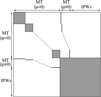
Figure 1: Illustration of the Coulomb matrix after transforming the MPB as described in the text. The elements that are in general nonzero are marked. The matrix is predominantly block-diagonal: for each atom and $LM$ channel there is one block of multipole-free MT functions $(\mu=0)$ and a larger block for the combined set of IPWs and MT functions with a nonvanishing multipole moment $(\mu\neq 0).$ Additionally, there are very few off-diagonal elements between MT functions with $\mu=0$ and $\mu\neq 0$.

III.4 Symmetry

Spatial and time-reversal symmetries are exploited to accelerate the code in three ways: (1) inversion symmetry leads to real-valued quantities. (2) If the wave functions $\varphi_{n\mathbf{k}}^{\sigma}$ and $\varphi_{n^{\prime}\mathbf{k}}^{\sigma}$ in Eq. (21) fall into different irreducible representations, the corresponding exchange matrix element vanishes. This can be used as a criterion whether an element must be calculated explicitly or not. And (3), for each $\mathbf{k}$ chosen from the irreducible wedge of the BZ the $\mathbf{q}$ summation in Eq. (21) is restricted to a smaller set of Bloch vectors giving rise to an extended irreducible BZ.

In general, the Coulomb matrix in Eq. (22) is Hermitian. If the system exhibits inversion symmetry and the MPB functions fulfill the condition $f(-\mathbf{r})=f^{*}(\mathbf{r})$, it becomes real-symmetric. Similarly, the vectors in Eq. (21) are then real instead of complex. This reduces the computational demand in terms of both CPU time and memory considerably. However, presently the condition only holds for the IPWs but not for the MT functions. We thus combine the MT functions of each pair of atoms $a$ and $-a$, which are related via inversion symmetry

$$M_{aLMP}^{\prime\mathbf{k}}(\mathbf{r})$$

$$= \frac{1}{\sqrt{2}}\left[M_{aLMP}^{\mathbf{k}}(\mathbf{r})+\left(-1\right)^{L+M}M_{(-a)L(-M)P}^{\mathbf{k}}(\mathbf{r})\right]$$

$$M_{(-a)L(-M)P}^{\prime\mathbf{k}}(\mathbf{r})$$

$$= \frac{i}{\sqrt{2}}\left[M_{aLMP}^{\mathbf{k}}(\mathbf{r})-\left(-1\right)^{L+M}M_{(-a)L(-M)P}^{\mathbf{k}}(\mathbf{r})\right]\,.$$

If the atom is placed in the origin, i.e., the atom indices $a$ and $-a$ correspond to the same atom, the transformation in Eq. (25) only holds for the integer index $M<0$, and we define

$$M_{aL0P}^{\prime\mathbf{k}}(\mathbf{r}) = \left\{\begin{array}[]{ll}\hphantom{ii\cdot}M_{aL0P}^{\mathbf{k}}(\mathbf{r})\,,&\mbox{if}\,L\,\,\mbox{even}\\ i\cdot M_{aL0P}^{\mathbf{k}}(\mathbf{r})\,,&\mbox{if}\,L\,\,\mbox{odd}\end{array}\right.$$ (28)

for $M=0$. It is then easy to show that the transformed functions will fulfill the condition above. We note that this symmetrization leaves the form of the Coulomb matrix, as shown in Fig. 1, intact.

The great orthogonality theorem of group theory demands that the matrix elements $\langle\varphi_{n\mathbf{k}}^{\sigma}|A|\varphi_{n^{\prime}\mathbf{k}}^{\sigma}\rangle$ of any operator $A$, which commutes with the symmetry operations of the system, are zero, if the wave functions fall into different irreducible representations. In particular, this holds for the exchange operator in Eq. (7). Unfortunately, the irreducible representations are not available in our DFT code and their evaluation in each iteration would be computationally expensive. Instead, we exploit the fact that the great orthogonality theorem applies to any operator that has the full symmetry of the system. A suitable operator is given by

$$\Theta^{\mathrm{MT}}(\mathbf{r}) = 1-\Theta(\mathbf{r})\,.$$ (29)

The calculation of its matrix elements $\langle\varphi_{n\mathbf{k}}^{\sigma}|\Theta^{\mathrm{MT}}|\varphi_{n^{\prime}\mathbf{k}}^{\sigma}\rangle$ is elementary and takes negligible CPU time. If the matrix elements between two groups of degenerate wave functions are numerically zero, we conclude that these two groups belong to different irreducible representations. Then the corresponding matrix elements of the nonlocal exchange potential in Eq. (21) must be zero, too. The question remains whether, conversely, the matrix elements of Eq. (29) are always nonzero, if the two irreducible representations are identical. This is not fulfilled in only two cases. First, either of the two wave functions is completely confined to the MT sphere. This can be ruled out since we deal with valence or conduction states. Second, the matrix elements are zero by accident: the overlaps in the interstitial and the MT spheres exactly cancel. However, this is extremely unlikely, verging on the impossible. We find that the procedure provides a fast and reliable criterion to decide in advance, which exchange matrix elements are nonzero and must be calculated explicitly. In this way we again save computation time.

In general, if a symmetry operation, which leaves the Hamiltonian invariant, acts on a wave function, it generates another wave function with the same energy. In other words, the solutions of the one-particle equations at two different $\mathbf{k}$ points are equivalent, if the $\mathbf{k}$ vectors are related by a symmetry operation. This can be used to restrict the set of $\mathbf{k}$ points, at which the Hamiltonian must be diagonalized, to a smaller set, whose members are not pairwise related. This defines the so-called irreducible Brillouin zone (IBZ), which is routinely employed in calculations with periodic boundary conditions. In a similar way, the summation over $\mathbf{q}$ points in the nonlocal exchange term can be confined, too. However, due to the additional dependence on $\mathbf{k}$ and $\mathbf{k}$$-$$\mathbf{q}$, we can only employ those symmetry operations $P_{i}^{\mathbf{k}}$ that leave the given $\mathbf{k}$ vector invariant, i.e., $P_{i}^{\mathbf{k}}\mathbf{k}=\mathbf{k}+\mathbf{G}_{i}^{\mathbf{k}}$, where $\mathbf{G}_{i}^{\mathbf{k}}$ is a reciprocal lattice vector. This subset of operations $\{P_{i}^{\mathbf{k}}\}$ is commonly called little group $\mathrm{LG(\mathbf{k})}$. In the same way as for the IBZ the little group gives rise to a minimal set of inequivalent $\mathbf{q}$ points, which we denote by the extended IBZ $[\mathrm{EIBZ}(\mathbf{k})]$. Leaving out here in the paper the description of nonsymmorphic and time-reversal symmetries for simplicity, the exchange potential in the LAPW basis can then be written as

$$V_{\mathrm{x,\mathbf{G}\mathbf{G}^{\prime}}}^{\mathrm{NL},\sigma}(\mathbf{k}) = -\sum_{i}^{\mathrm{LG}(\mathbf{k})}\sum_{\mathbf{q}}^{\mathrm{EIBZ}(\mathbf{k})}\frac{1}{N_{\mathbf{k},\mathbf{q}}}\sum_{n}^{\mathrm{occ.}}\iint\frac{\chi_{\mathbf{k}\mathbf{G}}^{\sigma*}(\mathbf{r})[P_{i}^{\mathbf{k}^{{\scriptstyle-1}}}\varphi_{n\mathbf{k}-\mathbf{q}}^{\sigma}(\mathbf{r})][P_{i}^{\mathbf{k}^{{\scriptstyle-1}}}\varphi_{n\mathbf{k}-\mathbf{q}}^{\sigma*}(\mathbf{r}^{\prime})]\chi_{\mathbf{k}\mathbf{G}^{\prime}}^{\sigma}(\mathbf{r}^{\prime})}{|\mathbf{r}-\mathbf{r}^{\prime}|}d^{3}r\,d^{3}r^{\prime}$$ (30)

$$= -\sum_{i}^{\mathrm{LG}(\mathbf{k})}\sum_{\mathbf{q}}^{\mathrm{EIBZ}(\mathbf{k})}\frac{1}{N_{\mathbf{k},\mathbf{q}}}\sum_{n}^{\mathrm{occ.}}\iint\frac{\chi_{\mathbf{k}(P_{i}^{\mathbf{k}}\mathbf{G}+\mathbf{G}_{i}^{\mathbf{k}})}^{\sigma*}(\mathbf{r})\varphi_{n\mathbf{k}-\mathbf{q}}^{\sigma}(\mathbf{r})\varphi_{n\mathbf{k}-\mathbf{q}}^{\sigma*}(\mathbf{r}^{\prime})\chi_{\mathbf{k}(P_{i}^{\mathbf{k}}\mathbf{G}^{\prime}+\mathbf{G}_{i}^{\mathbf{k}})}^{\sigma}(\mathbf{r}^{\prime})}{|\mathbf{r}-\mathbf{r}^{\prime}|}d^{3}r\,d^{3}r^{\prime}\,,$$

where $N_{\mathbf{k},\mathbf{q}}$ is the number of symmetry operations that are members of both $\mathrm{LG(\mathbf{k})}$ and $\mathrm{LG(\mathbf{q})}$. As a result, we can restrict the $\mathbf{q}$ summation to the $\mathrm{EIBZ}(\mathbf{k})$ and add the contribution of all other $\mathbf{q}$ points by transforming the final matrix with the operations $\mathrm{LG}(\mathbf{k})$ and summing. This takes very little computation time because a symmetry operation acts as a one-to-one mapping in the space of the augmented plane waves as indicated in Eq. (30). Local orbitals transform in a similar way. This is why we apply the symmetrization to $V_{\mathrm{x},\mathbf{G}\mathbf{G}^{\prime}}^{\mathrm{NL},\sigma}$ instead of $V_{\mathrm{x},nn^{\prime}}^{\mathrm{NL},\sigma}$, in which case we would need the irreducible representations again. We note that the whole formalism can be easily extended to the case of nonsymmorphic and time-reversal symmetry operations.

In summary, we compute the nonlocal exchange potential $V_{\mathrm{x},nn^{\prime}}^{\mathrm{NL},\sigma}(\mathbf{k})$ in the space of the wave functions, where we restrict the $\mathbf{q}$ summation to the $\mathrm{EIBZ}(\mathbf{k})$ and evaluate only those band combinations $n$ and $n^{\prime}$, which can be expected to be nonzero. We then apply the transformation in Eq. (11) and sum up the different matrix elements according to Eq. (30).

III.5 Singularity of the Coulomb matrix

Due to the long-range nature of the Coulomb interaction the matrix $v_{IJ}(\mathbf{q})$, Eq. (22), is singular at $\mathbf{q}=0$, which leads to a divergent integrand in Eq. (21). As the divergence is proportional to $1/q^{2}$, a three-dimensional integration over the BZ yields a finite value. However, in a practical calculation the $\mathbf{q}$ summation in Eq. (21) is not an integral but a weighted sum over the discrete BZ mesh. A simple way to avoid the divergence is to exclude the point $\mathbf{q}=\mathbf{0}$ from the $\mathbf{k}$-point set. Then all terms in Eq. (21) are finite and the $\mathbf{q}$ sum can be evaluated easily. We find that this leads to very poor convergence with respect to the BZ sampling because the quantitatively important region around $\mathbf{q}=\mathbf{0}$ is not properly taken into account. Hence, it is advantageous to explicitly treat the $\Gamma$ point and the singularity of the Coulomb matrix there. This is possible by a decomposition of $v_{IJ}(\mathbf{q})$ into a divergent and a nondivergent part(Friedrich, )

$$v_{IJ}(\mathbf{q})=\frac{4\pi}{V}\frac{1}{q^{2}}\langle\tilde{M}_{I}^{\mathbf{q}}|e^{i\mathbf{q}\cdot\mathbf{r}}\rangle\langle e^{i\mathbf{q}\cdot\mathbf{r}}|\tilde{M}_{J}^{\mathbf{q}}\rangle+v_{IJ}^{\prime}(\mathbf{q})\,.$$ (31)

The second term is finite. Its long-wavelength limit replaces the matrix $v_{IJ}(\mathbf{0})$ in Eq. (21) such that the $\mathbf{q}$ summation can be performed numerically. The divergent first term is given exactly in the limit $\mathbf{q}\rightarrow\mathbf{0}$ because the MPB contains the constant basis function explicitly (see Sec. III.2). Therefore, we may switch to a representation with the plane waves $e^{i\mathbf{q}\cdot\mathbf{r}}$. The contribution of the divergent term is then given by

$$\left.V_{\mathrm{x,}nn^{\prime}}^{\mathrm{NL},\sigma}(\mathbf{k})\right|_{\mathrm{div}} = -\frac{1}{2\pi^{2}}\left(\sum_{n^{\prime\prime}}^{\mathrm{occ.}}\int_{\mathrm{BZ}}\langle\varphi_{n\mathbf{k}}^{\sigma}|\varphi_{n^{\prime\prime}\mathbf{k}-\mathbf{q}}^{\sigma}e^{i\mathbf{q}\cdot\mathbf{r}}\rangle\frac{1}{q^{2}}\right.$$ (32)

$$\left.\times\langle e^{i\mathbf{q}\cdot\mathbf{r}}\varphi_{n^{\prime\prime}\mathbf{k}-\mathbf{q}}^{\sigma}|\varphi_{n^{\prime}\mathbf{k}}^{\sigma}\rangle d^{3}q-\mathrm{d.c.}\vphantom{\frac{1}{q^{2}}}\right),$$

where $\mathrm{d.c.}$ denotes a double-counting correction for the finite $\mathbf{q}$ points (see below). For the important region close to $\mathbf{q}=\mathbf{0}$ we can replace $\langle\cdot|\cdot\rangle$ by $\delta_{nn^{\prime\prime}}$ and $\delta_{n^{\prime}n^{\prime\prime}}$, respectively. We leave out higher-order corrections here for simplicity and defer a refined treatment employing $\mathbf{k}\cdot\mathbf{p}$ perturbation theory to App. A. In order to perform the $q$ integration analytically, we replace $1/q^{2}$ by the function

$$F(\mathbf{q}) = \sum_{\mathbf{G}}\frac{e^{-\beta|\mathbf{q}+\mathbf{G}|^{2}}}{|\mathbf{q}+\mathbf{G}|^{2}}\,,$$ (33)

which was proposed by Massidda et al. in Ref. Hartree-Fock_LAPW_approach_to_the_electronic_properties_of_periodic_systems, . The parameter $\beta>0$ ensures that the BZ integral can be extended over the whole reciprocal space. In contrast to Ref. Hartree-Fock_LAPW_approach_to_the_electronic_properties_of_periodic_systems, we choose this parameter as small as possible such that Eq. (33) is sufficiently close to $1/q^{2}$. Furthermore, by this choice terms arising from the product of $1/q^{2}$ with the first-order term of the exponential function are small and can thus be neglected. After inserting Eq. (33) in Eq. (32) we obtain

$$\left.V_{\mathrm{x,}nn^{\prime}}^{\mathrm{NL},\sigma}(\mathbf{k})\right|_{\mathrm{div}} = -\delta_{nn^{\prime}}f_{n\mathbf{k}}^{\sigma}\left(\frac{1}{2\pi^{2}}\int\frac{e^{-\beta|\mathbf{q}|^{2}}}{q^{2}}d^{3}q\vphantom{\frac{1}{N_{\mathbf{k}}\Omega}\sum_{q\neq 0}}\right.$$ (34)

$$\left.-\frac{1}{N_{\mathbf{k}}\Omega}\sum_{q\neq 0}\frac{e^{-\beta|\mathbf{q}|^{2}}}{q^{2}}\right)\,,$$

where the summation over $q\neq 0$ avoids double counting, $N_{\mathbf{k}}$ denotes the number of $\mathbf{k}$ points, and $f_{n\mathbf{k}}^{\sigma}$ is the occupation number. In order to evaluate the integral and sum we introduce a reciprocal cutoff radius $q_{0}$ and finally obtain

$$\left.V_{\mathrm{x,}nn^{\prime}}^{\mathrm{NL},\sigma}(\mathbf{k})\right|_{\mathrm{div}} = -\delta_{nn^{\prime}}f_{n\mathbf{k}}^{\sigma}\left(\frac{1}{\sqrt{\pi\beta}}\,\mathrm{erf}\left(\sqrt{\beta}q_{0}\right)\vphantom{\frac{1}{N_{\mathbf{k}}\Omega}\sum_{0<q\leq q_{0}}}\right.$$ (35)

$$\left.-\frac{1}{N_{\mathbf{k}}\Omega}\sum_{0<q\leq q_{0}}\frac{e^{-\beta|\mathbf{q}|^{2}}}{q^{2}}\right)\,.$$

We get rid off the convergence parameter $q_{0}$ by relating $\beta$ and $q_{0}$ by $e^{-\beta q_{0}^{2}}=\beta$. We find that $\beta=0.005$ is a good choice.

Figure 2 shows the convergence of the exchange energy $E_{\mathrm{x}}^{\mathrm{NL}}=2\sum_{n\mathbf{k}}^{\mathrm{occ.}}V_{\mathrm{x},nn}^{\mathrm{NL}}(\mathbf{k})$ with respect to the $\mathbf{k}$-point sampling for NaCl. While the separate contributions from the divergent term, Eq. (35), and the remainder converge poorly, their sum nearly look constant on the energy scale of Fig. 2(a). As shown in Fig. 2(b), the $\mathbf{k}$-point convergence can be improved further by taking corrections at $\mathbf{q}=\mathbf{0}$ into account that arise from multiplying $1/q^{2}$ with second-order terms of $\langle\cdot|\cdot\rangle\langle\cdot|\cdot\rangle$ derived by $\mathbf{k}\cdot\mathbf{p}$ perturbation theory (see App. A).

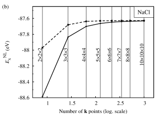
Figure 2: (a) Exchange energy as a function of the $\mathbf{k}$-point mesh for NaCl. The dashed and dotted curves correspond to the divergent contribution Eq. (35) and the remaining numerical sum, respectively. The sum of both is shown by the solid curve. (b) Convergence of the exchange energy with (dashed curve) and without (solid curve) higher-order corrections at $\mathbf{q}=\mathbf{0}$. Please note the different scale of the exchange energy in figures (a) and (b).

IV Calculations

We have implemented the above algorithm in the fleur program package.(Fleur, ) We take the MT functions $u_{l0}^{a\sigma}(r)$ of Eq. (9) as the solutions of the radial Kohn-Sham equation with the local effective potential derived from the full PBE functional and $u_{l1}^{a\sigma}(r$) as their energy derivatives. If necessary local orbitals are employed to describe semicore states.(Local_Orbitals1, ; Local_Orbitals2, ) In the calculations presented here, the core states are taken from a preceding PBE calculation and kept fixed during the self-consistent-field cycle with the PBE0 hybrid functional.

Figure 3: Convergence behavior of the electron density for Si in a self-consistent-field cycle. The solid and dashed curves correspond to calculations with and without the nested density convergence scheme (see text).

The one-particle Eq. (10) must be solved self-consistently, as its local and nonlocal potentials depend on the electron density and density matrix, respectively, and thus on the solution of wave functions determined in Eq. (10). Input and output densities must coincide in self-consistency. As a measure of convergence one usually considers the root-mean square of the difference between the input and output densities $\Delta n$, measured in $\mathrm{me/bohr}^{3}$, where $\mathrm{e}$ is the elementary charge. We consider a calculation converged, if this value falls below $10^{-5}\,\mathrm{me/bohr}^{3}$. A straight iterative solution of the one-particle equation is bound to diverge. In DFT calculations with a conventional local functional it is required to construct a new charge density for the upcoming self-consistency cycle from the current and a history of previous densities, as for example, in the standard simple-mixing and Broyden-mixing schemes.Broyden1 ; Broyden2 However, in addition to the local effective potential Eq. (10) contains a nonlocal potential, which depends on the density matrix for which no similarly simple mixing procedure is available. Indeed, we find that a standard density mixing leads to poor convergence: $27$ iterations for $\mathrm{Si}$, as illustrated in Fig. 3, and more than $200$ iterations for $\mathrm{SrTiO}_{3}$ are necessary. On the other hand, the fact that in the FLAPW method the basis for the wave functions - and hence for the density matrix - depends on the potential and changes in each iteration in contrast to that for the density makes the definition of a mixing scheme for the density matrix difficult, if not impossible. Therefore, we employ an alternative pragmatic approach, which leads to a surprisingly fast density convergence for all systems treated so far. The self-consistency cycle is divided into an outer iteration of the density matrix and an inner self-consistency step of the density. After the construction of the nonlocal exchange potential we keep its matrix representation $V_{\mathrm{x},\mathbf{G}\mathbf{G}^{\prime}}^{\mathrm{NL}}$ fixed and iterate Eq. (10) until self-consistency in the density is reached; only then the exchange potential $V_{\mathrm{x},\mathbf{G}\mathbf{G}^{\prime}}^{\mathrm{NL}}$ is updated from the current wave functions, which starts a new set of inner self-consistency iterations. With this nested iterative procedure the outer loop converges after eight steps for $\mathrm{Si}$, see Fig. 3, and after only twelve steps for $\mathrm{SrTiO}_{3}$. One iteration of the inner loop lasts only $1.0\,\mathrm{s}$ for $\mathrm{Si}$ and $8.3\,\mathrm{s}$ for $\mathrm{SrTiO}_{3}$ on a single Intel Xeon X5355 at 2.66 GHz (Cache 4 MB) using a 4$\times$4$\times$4 $\mathbf{k}$-point set. This is negligible compared with the cost for the construction of the nonlocal potential in the outer loop, which takes $11.9\,\mathrm{s}$ for $\mathrm{Si}$ and $573.1\,\mathrm{s}$ for $\mathrm{SrTiO_{3}}$.

In the following we discuss the convergence of single-particle excitation energies and total energy differences with respect to the cutoff parameters $L_{\mathrm{max}}$ and $G^{\prime}_{\mathrm{max}}$ for the MPB as well as the number of bands $n_{\mathrm{max}}$, which are used to represent the nonlocal exchange potential. In Figs. 4(a) and 4(b) we show the behavior of the excitation energies of the transitions $\Gamma_{25^{\prime}v}\rightarrow\Gamma_{15c}$ and $\Gamma_{25^{\prime}v}\rightarrow\mathrm{X}_{1c}$ for $\mathrm{Si}$ as well as $\Gamma_{15v}\rightarrow\Gamma_{25^{\prime}c}$ and $\mathrm{R}_{15^{\prime}v}\rightarrow\mathrm{R}_{25^{\prime}c}$ for $\mathrm{SrTiO}_{3}$ obtained from the self-consistent solution of Eq. (10) as functions of the convergence parameters. The diagrams show that the convergence of these transition energies to within $0.01\,\mathrm{eV}$ is achieved for $G^{\prime}_{\mathrm{max}}=2.0\,\mathrm{bohr}^{-1}$ and $G^{\prime}_{\mathrm{max}}=2.7\,\mathrm{bohr}^{-1}$ for $\mathrm{Si}$ and $\mathrm{SrTiO}_{3}$, respectively. This is well below the exact limit $G^{\prime}_{\mathrm{max}}=2G_{\mathrm{max}}$ for the wave-function products ($G_{\mathrm{max}}=3.6\,\mathrm{bohr}^{-1}$ for $\mathrm{Si}$ and $G_{\mathrm{max}}=4.3\,\mathrm{bohr}^{-1}$ for $\mathrm{SrTiO}_{3}$). It is even below the reciprocal cutoff radius $G_{\mathrm{max}}$ for the wave functions themselves. The same can be said about the cutoff parameter $L_{\mathrm{max}}$ for the angular momentum. Figures 4(a) and 4(b) show that for both materials $L_{\mathrm{max}}=4$ is sufficient while the representation of wave functions that are properly matched at the MT boundaries requires a much larger cutoff value of $l_{\mathrm{max}}=8$. A similar behavior was found for GW calculations employing the MPB.(GW-Fleur, ) The number of bands $n_{\mathrm{max}}$ that define the Hilbert space in which the exchange potential is represented can be restricted to only $50$ bands per atom, which amounts to 100 and 250 bands for $\mathrm{Si}$ and $\mathrm{SrTiO}_{3}$, respectively.

Figure 4(c) shows that the total energy difference between the diamond and wurtzite structures of $\mathrm{Si}$ converges even faster than the transition energies above. With a reciprocal cutoff radius of $G^{\prime}_{\mathrm{max}}=2.25\,\mathrm{bohr^{-1}}$, an angular-momentum cutoff of $L_{\mathrm{max}}=4$ and $20$ bands per atom we achieve an accuracy of $1\,\mathrm{meV}$, which is one order of magnitude smaller than the tolerance for the transition energies and well below the error resulting from the BZ discretization of the 4$\times$4$\times$4 $\mathbf{k}$-point set. The calculations are converged to within $2\,\mathrm{meV}$ with a 8$\times$8$\times$8 mesh, with which the diamond structure is $112\,\mathrm{meV}$ lower in energy than the wurtzite structure. This is very close to the total energy difference of $92\,\mathrm{meV}$ obtained with the PBE functional.

Figure 4: (a) Convergence of the $\Gamma_{25^{\prime}v}\rightarrow\Gamma_{15c}$ (solid line, left scale) and $\Gamma_{25^{\prime}v}\rightarrow\mathrm{X}_{1c}$ (dashed line, right scale) transitions for $\mathrm{Si}$, (b) of the direct (solid line, left scale) and indirect band gaps (dashed line, right scale) of $\mathrm{SrTiO_{3}}$, and (c) the total energy difference $\Delta E$ between the diamond (dia) and wurtzite (wz) phases of Si ($\Delta E=E_{\mathrm{wz}}-E_{\mathrm{dia}}$) with respect to the reciprocal cutoff value $G_{\mathrm{max}}^{\prime}$ and the angular momentum cutoff $L_{\mathrm{max}}$ for the MPB, as well as the number of bands per atom used to construct the exchange potential in the space of the wave functions. For these convergence tests we employ a 4$\times$4$\times$4 $\mathbf{k}$-point set. See Tables 1 and 2 and the text for the fully converged values.

For the materials treated so far we find that $G^{\prime}_{\mathrm{max}}$ can be chosen universally smaller than $G_{\mathrm{max}}$, $G^{\prime}_{\mathrm{max}}=0.75\,G_{\mathrm{max}}$ as a rule of thumb, while the cutoff parameter $L_{\mathrm{max}}$ is more material specific. For example, for $\mathrm{EuO}$, whose spin-polarized valence and conduction states are formed by $f$ electrons, the larger value of $L_{\mathrm{max}}=6$ is necessary for proper convergence, which is still below $l_{\mathrm{max}}=8$, though. Likewise, the optimal number of states $n_{\mathrm{max}}$ is material specific, and thorough convergence tests are again necessary.

For reference, we show transition energies obtained with the PBE0 hybrid functional for $\mathrm{Si}$, $\mathrm{C}$, $\mathrm{GaAs}$, $\mathrm{MgO}$, $\mathrm{NaCl}$, and crystalline $\mathrm{Ar}$ in Table 1. All calculations are performed at the experimental lattice constant with a 12$\times$12$\times$12 $\mathbf{k}$-point mesh. The PBE0 values are converged to within $0.01\,\mathrm{eV}$ with respect to the convergence parameters $G^{\prime}_{\mathrm{max}}$, $L_{\mathrm{max}}$, and $n_{\mathrm{max}}$. We also list the PBE values and a comparison with recent PAW calculations,(Screened_hybrid_density_functionals_apllied_to_solids, ) with which we find an overall good agreement; for $\mathrm{Si}$ and $\mathrm{GaAs}$ the values are nearly identical. There are slightly larger discrepancies for systems with wider band gaps, which we attribute to the different basis sets, because the corresponding PBE values show similar deviations, too. In all cases the admixture of exact HF exchange leads to an increase in the transition energies in such a way that they come close to the measured values. For the materials shown in Table 1 there is still a slight underestimation of the band gaps for insulators and an overestimation for semiconductors.

Table 1: PBE and PBE0 transition energies in eV for Si, C, GaAs, MgO, NaCl, and Ar compared with theoretical and experimental values from the literature. All results are obtained with a 12$\times$12$\times$12 $\mathbf{k}$-point set.

		This work		$\mathrm{PAW^{a}}$		Expt.
		PBE	PBE0	PBE	PBE0
Si	$\Gamma\rightarrow\Gamma$	2.56	3.96	2.57	3.97	$3.4^{b}$
	$\Gamma\rightarrow\mathrm{X}$	0.71	1.93	0.71	1.93	—
	$\Gamma\rightarrow\mathrm{L}$	1.54	2.87	1.54	2.88	$2.4^{b}$
C	$\Gamma\rightarrow\Gamma$	5.64	7.74	5.59	7.69	$7.3^{b}$
	$\Gamma\rightarrow\mathrm{X}$	4.79	6.69	4.76	6.66	—
	$\Gamma\rightarrow\mathrm{L}$	8.58	10.88	8.46	10.77	—
GaAs	$\Gamma\rightarrow\Gamma$	0.55	2.02	0.56	2.01	$1.63^{b}$
	$\Gamma\rightarrow\mathrm{X}$	1.47	2.69	1.46	2.67	$2.18^{b},2.01^{b}$
	$\Gamma\rightarrow\mathrm{L}$	1.02	2.38	1.02	2.37	$1.84^{b}$,$1.85^{b}$
MgO	$\Gamma\rightarrow\Gamma$	4.84	7.31	4.75	7.24	$7.7^{c}$
	$\Gamma\rightarrow\mathrm{X}$	9.15	11.63	9.15	11.67	—
	$\Gamma\rightarrow\mathrm{L}$	8.01	10.51	7.91	10.38	—
NaCl	$\Gamma\rightarrow\Gamma$	5.08	7.13	5.20	7.26	$8.5^{d}$
	$\Gamma\rightarrow\mathrm{X}$	7.39	9.59	7.60	9.66	—
	$\Gamma\rightarrow\mathrm{L}$	7.29	9.33	7.32	9.41	—
Ar	$\Gamma\rightarrow\Gamma$	8.71	11.15	8.68	11.09	$14.2^{e}$

aReference Screened_hybrid_density_functionals_apllied_to_solids,		bReference Landolt-Boernstein,		cReference Adachi,
dReference NaCl,		eReference Ar,

In contrast to DFT calculations with a purely local effective potential the nonlocality of the exchange potential does not allow a straightforward calculation of band structures, i.e., a diagonalization of the Hamiltonian at an arbitrary point $\mathbf{k}$ in the BZ because according to Eq. (21) the construction of $V_{\mathrm{x}}^{\mathrm{NL},\sigma}(\mathbf{k})$ would require the knowledge of all occupied states at the points $\mathbf{k}$$-$$\mathbf{q}$, where $\mathbf{q}$ is an element of the $\mathbf{k}$ mesh defined in Sec. III.3. However, these wave functions are, in general, unknown. Therefore, we employ the Wannier-interpolation technique(Wannier, ; Wannier_entangled, ; Wannier-FLAPW, ) as realized in the wannier90 code(Wannier90, ) to interpolate the band energies between the ones of the $\mathbf{k}$ mesh. As an example Fig. 5 shows the PBE and the interpolated PBE0 band structure for $\mathrm{Si}$, which was constructed with the help of eight $\mathrm{sp}{}^{3}$-like maximally localized Wannier orbitals from the four valence and the four lowest conduction bands. The comparison shows that the main effect of the nonlocal exchange potential is an upwards shift of the conduction bands while the band dispersion remains relatively unchanged. There is, however, a clear increase in the occupied band width. As in the case of PBE the conduction-band minimum lies at a point close to but not exactly at the X point. The plot of the interpolated band structure thus allows to determine the fundamental PBE0 band gap of Si easily, which amounts to $1.74\,\mathrm{eV}$. It overestimates the experimental value of $1.17\,\mathrm{eV}$ (Ref. Landolt-Boernstein, ) while the PBE value of $0.47\,\mathrm{eV}$ underestimates it.

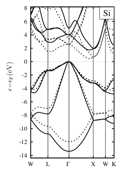
Figure 5: Comparison of the PBE (dotted lines) and the Wannier-interpolated PBE0 band structure (solid lines) for Si. Energy $\epsilon$ is given with respect to the Fermi energy $\epsilon_{\textrm{F}}$.

We finally apply the PBE0 functional to the more complex oxides $\mathrm{ZnO}$, $\mathrm{SrTiO}_{3}$, $\alpha$-$\mathrm{Al}_{2}\mathrm{O}_{3}$, and $\mathrm{EuO}$. The resulting band gaps are given in Table 2.

Table 2: PBE and PBE0 transition energies in eV for ZnO, $\mathrm{SrTiO}_{3}$, $\mathrm{Al}_{2}\mathrm{O}_{3}$, and EuO. All results are obtained with a 8$\times$8$\times$8 $\mathbf{k}$-point set.

		PBE	PBE0	Expt.
ZnO	$\Gamma\rightarrow\Gamma$	0.94	3.32	$3.44^{a}$
$\mathrm{SrTiO}_{3}$	$\Gamma\rightarrow\Gamma$	2.19	4.39	$3.75^{b}$
	$\mathrm{R}\rightarrow\mathrm{\Gamma}$	1.83	4.02	$3.25^{b}$
$\mathrm{Al}_{2}\mathrm{O}_{3}$	$\Gamma\rightarrow\Gamma$	6.52	9.12	$8.8^{c},9.5^{d}$
EuO	$\Gamma\rightarrow\mathrm{X}$	—	1.31	$0.9^{e}$

aReference ZnO-dbands,		bReference STO-bandgap,		cReference Al2O3-2,
dReference Al2O3-1,		eReference EuO-FMbandgap,

For the II-VI semiconductor $\mathrm{ZnO}$ it is well known that LDA and GGA not only underestimate the band gap but also yield wrong occupied $d$ band positions;(ZnO_Sic, ) they are about $3\,\mathrm{eV}$ too high in energy compared with experiment. As a consequence the $\mathrm{Zn}$ $d$ states hybridize strongly with the $\mathrm{O}$ $p$ states. The wrong $d$ band position relative to the $p$ states is commonly attributed to the unphysical self-interaction error present in LDA and GGA, which is larger for localized than for delocalized electrons. The admixture of exact HF exchange into the hybrid functionals partly cancels this error and should therefore lower the relative $d$ band position. Figure 6 shows the density of states for PBE (lower panel) and PBE0 (upper panel) again obtained from a Wannier-interpolated denser $\mathbf{k}$-point mesh. In fact, the self-interaction correction leads to a substantially stronger binding of the Zn $d$ states from $5.1\,\mathrm{eV}$ in PBE to $6.3\,\mathrm{eV}$ in PBE0 whereas the experimental value is $7.8\,\mathrm{eV}$.(ZnO-dbands, ) (The values correspond to the center of gravity of the $d$ bands.) Concomitantly the $d$$-$$p$ hybridization becomes less pronounced leading to an increase of the $\mathrm{O}$ $p$ valence band width from $4.2\,\mathrm{eV}$ in PBE to $5.2\,\mathrm{eV}$ in PBE0, which deviates from the experimental value(ZnO-dbands, ) by only $0.1\,\mathrm{eV}$. Incidentally, we also observe a stronger binding of the $d$ electrons in $\mathrm{Ge}$ and $\mathrm{GaAs}$.

Figure 6: Comparison of the PBE and PBE0 density of states (DOS) for ZnO. The stronger binding of the Zn $d$ electrons in PBE0 is evident. Energy $\epsilon$ is given with respect to the Fermi energy $\epsilon_{\textrm{F}}$.

The missing self-interaction correction in LDA and GGA affects the calculation of $f$-electron systems even more strongly. Ferromagnetic $\mathrm{EuO}$ is predicted to be metallic, while experimentally it is semiconducting with a nearly 100% spin-polarized conduction band,(EuO-Steeneken, ) a property which makes $\mathrm{EuO}$ an efficient spin-filter.(EuO-Moodera, ; EuO-Mueller, ) LDA+U has been shown to give the correct electronic structure, if the U parameters are chosen properly.(EuO-LDA+U, ; EuO-Elfimov, ) We find that the parameter-free PBE0 hybrid functional also gives the physically correct semiconducting behavior for ferromagnetic EuO even though the calculation was started from the metallic ground state obtained from PBE. The resulting ferromagnetic semiconductor exhibits a theoretical band gap of $1.31\,\mathrm{eV}$, which slightly overestimates the experimental value of $0.9\,\mathrm{eV}$.(EuO-FMbandgap, ) The exchange splitting of the conduction band amounts to $1.02\,\mathrm{eV}$ whereas experimental measurements give $0.6\,\mathrm{eV}$.(EuO-Steeneken, ) In summary, the parameter-free PBE0 hybrid functional correctly predicts the electronic ground state of ferromagnetic EuO in contrast to LDA and GGA.

V Summary

We have presented an implementation of the PBE0 hybrid functional within the all-electron FLAPW method as realized in the fleur code.(Fleur, ) The computationally most demanding step in the numerical procedure is the calculation of the nonlocal exact exchange term, which is a central ingredient of hybrid functionals. Our implementation relies on the matrix representation of the Coulomb potential in an auxiliary mixed product basis, which is constructed from products of the FLAPW basis functions. The nonlocal exchange integrals then decompose into vector-matrix-vector products. The computational cost for these products is considerably reduced by a suitable unitary transformation of the mixed product basis, which makes the Coulomb matrix sparse. If inversion symmetry is present, the mixed product basis can be defined in such a way that the Coulomb matrix and the vectors become real-valued, which again gives rise to a speedup of the code. Spatial and time-reversal symmetries are further exploited (1) to identify those exchange matrix elements in advance that are zero and need not to be calculated, and (2) to restrict the $\mathbf{k}$-point summation for the nonlocal quantity to an irreducible wedge of the BZ.

We have demonstrated that the PBE0 interband transition and total energies converge quickly with respect to the parameters of the MPB. Thus, the MPB provides a small but accurate all-electron basis for the construction of the exchange potential. We have shown that while a direct iteration of the generalized Kohn-Sham one-particle equation needs extensively many steps to converge, a nested density-only and density-matrix iteration scheme accelerates the convergence of the self-consistent-field cycle considerably.

We confirm that the resulting PBE0 gap energies for a variety of semiconductors and insulators are consistently closer to experimental measurements than their PBE counterparts and compare very well with recent theoretical results(Screened_hybrid_density_functionals_apllied_to_solids, ) obtained with the PAW method. In addition, we have performed PBE0 calculations for the oxides $\mathrm{ZnO}$, $\mathrm{SrTiO}_{3}$, $\mathrm{Al}_{2}\mathrm{O}_{3}$, and $\mathrm{EuO}$. Again, the band gaps are clearly improved compared with PBE. Here we focused in particular on $\mathrm{ZnO}$ and $\mathrm{EuO}$, which contain $d$ and $f$ electrons, respectively. Due to the missing self-interaction correction conventional local xc functionals are known to fail in describing these localized states properly: the occupied $d$ band position of $\mathrm{ZnO}$ appear too high in energy while $\mathrm{EuO}$ is even incorrectly predicted to be a metal. The exact exchange potential of the PBE0 hybrid functional reduces this self-interaction error leading to an overall improved description of the relative energetic positions of the localized and delocalized states: the Zn $d$ bands are lowered in energy and thus come closer to their experimental position. The reduced $d$$-$$p$ hybridization leads to an increase of the $\mathrm{O}$ $p$ band width to $5.2\,\mathrm{eV}$, which is in good agreement with the experiment. Furthermore, in contrast to PBE the PBE0 hybrid functional correctly predicts a semiconducting ground state for ferromagnetic EuO. The band gap and the energy splitting are in satisfactory agreement with experiment.

We note that the numerical procedure presented in this paper is not pertinent to the PBE0 hybrid functional and can easily be used for any other hybrid functional that contains the exact exchange potential, e.g., for the popular B3LYP functional.(B3LYP, ) Furthermore, it allows a straightforward implementation of more general nonlocal potentials, e.g., the HSE functional,(HSE, ; HSE06, ) which is based on a screened Coulomb interaction. For this we just have to replace the Coulomb matrix [Eq. 22] by the matrix representation of the screened potential. We also note that in this case there is no divergence at the BZ center. The orbital-dependent Hartree-Fock term can also be used as part of an exchange-correlation functional (e.g., the exact-exchange functional) within the optimized-effective-potential (OEP) method.(OEP1, ; OEP2, ) There, a local instead of a nonlocal effective potential is derived, which requires the solution of the so-called OEP equation. In general, the nonlocal exchange term is the first term in an expansion of the xc functional with respect to the Coulomb interaction strength and thus a central ingredient in an systematic expansion of the xc functional.

Appendix A Terms of the BZ integrand beyond $1/q^{2}$

Figure 2(b) shows that the $\mathbf{k}$-point convergence can be improved considerably by taking into account terms of the integrand of Eq. (32) at $\mathbf{q}=0$ beyond the $1/q^{2}$ term

$$A_{\mathbf{k},n_{1}n_{2}}^{\sigma}(\mathbf{q}) = \sum_{n}\langle\varphi_{n_{1}\mathbf{k}}^{\sigma}|\varphi_{n\mathbf{k}-\mathbf{q}}^{\sigma}e^{i\mathbf{q}\cdot\mathbf{r}}\rangle\frac{1}{q^{2}}$$

$$\times\langle e^{i\mathbf{q}\cdot\mathbf{r}}\varphi_{n\mathbf{k}-\mathbf{q}}^{\sigma}|\varphi_{n_{2}\mathbf{k}}^{\sigma}\rangle-\delta_{n_{1},n_{2}}\frac{f_{n_{1},\mathbf{k}}^{\sigma}}{q^{2}}\,.$$

These terms arise from the expansion

$$\Phi_{n,\mathbf{k},\mathbf{q}}^{\sigma}(\mathbf{r}) = e^{-i\mathbf{q}\cdot\mathbf{r}}\varphi_{n,\mathbf{k}+\mathbf{q}}^{\sigma}(\mathbf{r})$$

$$= \varphi_{n,\mathbf{k}}^{\sigma}(\mathbf{r})+\mathbf{q}\cdot\nabla_{\mathbf{q}}\Phi_{n,\mathbf{k},\mathbf{q}}^{\sigma}(\mathbf{r})$$

$$+\frac{1}{2}\mathbf{q}^{\mathrm{T}}\cdot\nabla_{\mathbf{q}}\nabla_{\mathbf{q}}^{\mathrm{T}}\Phi_{n,\mathbf{k},\mathbf{q}}^{\sigma}(\mathbf{r})\cdot\mathbf{q}+O(q^{3}),$$

where

$$\nabla_{\mathbf{q}}\Phi_{n,\mathbf{k},\mathbf{q}}^{\sigma}(\mathbf{r})=-i\sum_{n^{\prime}\neq n}\frac{\langle\varphi_{n^{\prime},\mathbf{k}}^{\sigma}|\nabla|\varphi_{n,\mathbf{k}}^{\sigma}\rangle}{\epsilon_{n\mathbf{k}}^{\sigma}-\epsilon_{n^{\prime}\mathbf{k}}^{\sigma}}\varphi_{n^{\prime},\mathbf{k}}^{\sigma}(\mathbf{r})$$ (38)

is derived from $\mathbf{k}\cdot\mathbf{p}$ perturbation theory.(kp-historical, ) Inserting Eq. (A) into Eq. (A) and using

$$\langle\nabla_{\mathbf{q}}\nabla_{\mathbf{q}}^{\mathrm{T}}\Phi_{n_{1},\mathbf{k},\mathbf{q}}^{\sigma}|\varphi_{n_{2},\mathbf{k}}^{\sigma}\rangle+\langle\varphi_{n_{1},\mathbf{k}}^{\sigma}|\nabla_{\mathbf{q}}\nabla_{\mathbf{q}}^{\mathrm{T}}\Phi_{n_{2},\mathbf{k},\mathbf{q}}^{\sigma}\rangle\\ =-2\langle\nabla_{\mathbf{q}}\Phi_{n_{1},\mathbf{k},\mathbf{q}}^{\sigma}|\nabla_{\mathbf{q}}^{\mathrm{T}}\Phi_{n_{2},\mathbf{k},\mathbf{q}}^{\sigma}\rangle$$ (39)

inferred from the normalization of Eq. (A), we obtain

$$A_{\mathbf{k},n_{1}n_{2}}^{\sigma}(\mathbf{q})$$ (40)

$$= -\frac{1}{q}\left(\langle\nabla_{\mathbf{q}}\Phi_{n_{1},\mathbf{k},\mathbf{q}}^{\sigma}|\varphi_{n_{2},\mathbf{k}}^{\sigma}\rangle+\langle\varphi_{n_{1},\mathbf{k}}^{\sigma}|\nabla_{\mathbf{q}}\Phi_{n_{2},\mathbf{k},\mathbf{q}}^{\sigma}\rangle\right)\hat{\mathbf{q}}$$

$$+\hat{\mathbf{q}}^{\mathrm{T}}\left(\sum_{n}^{\mathrm{occ.}}\langle\varphi_{n_{1},\mathbf{k}}^{\sigma}|\nabla_{\mathbf{q}}\Phi_{n,\mathbf{k},\mathbf{q}}^{\sigma}\rangle\langle\nabla_{\mathbf{q}}^{\mathrm{T}}\Phi_{n,\mathbf{k},\mathbf{q}}^{\sigma}|\varphi_{n_{2},\mathbf{k}}^{\sigma}\rangle\right.$$

$$\left.\hphantom{\mathbf{q}^{T}(\sum}-\langle\nabla_{\mathbf{q}}\Phi_{n_{1},\mathbf{k},\mathbf{q}}^{\sigma}|\nabla_{\mathbf{q}}^{\mathrm{T}}\Phi_{n_{2},\mathbf{k},\mathbf{q}}^{\sigma}\rangle\vphantom{\sum_{n^{\prime}}^{\mathrm{occ.}}}\right)\hat{\mathbf{q}}$$

for $f_{n_{1},\mathbf{k}}^{\sigma}=f_{n_{2},\mathbf{k}}^{\sigma}=1$,

$$A_{\mathbf{k},n_{1}n_{2}}^{\sigma}(\mathbf{q}) = \hat{\mathbf{q}}^{\mathrm{T}}\left(\sum_{n}^{\mathrm{occ.}}\langle\varphi_{n_{1},\mathbf{k}}^{\sigma}|\nabla_{\mathbf{q}}\Phi_{n,\mathbf{k},\mathbf{q}}^{\sigma}\rangle\right.$$ (41)

$$\left.\times\langle\nabla_{\mathbf{q}}^{\mathrm{T}}\Phi_{n,\mathbf{k},\mathbf{q}}^{\sigma}|\varphi_{n_{2},\mathbf{k}}^{\sigma}\rangle\vphantom{\sum_{n}^{\mathrm{occ.}}}\right)\hat{\mathbf{q}}$$

for $f_{n_{1},\mathbf{k}}^{\sigma}=f_{n_{2},\mathbf{k}}^{\sigma}=0$, and

$$A_{\mathbf{k},n_{1}n_{2}}^{\sigma}(\mathbf{q})=-\frac{1}{q}\langle\nabla_{\mathbf{q}}\Phi_{n_{1},\mathbf{k},\mathbf{q}}^{\sigma}|\varphi_{n_{2},\mathbf{k}}^{\sigma}\rangle\hat{\mathbf{q}}$$

$$+\hat{\mathbf{q}}^{\mathrm{T}}\left(\sum_{n}^{\mathrm{occ.}}\langle\varphi_{n_{1},\mathbf{k}}^{\sigma}|\nabla_{\mathbf{q}}\Phi_{n,\mathbf{k},\mathbf{q}}^{\sigma}\rangle\times\langle\nabla_{\mathbf{q}}^{\mathrm{T}}\Phi_{n,\mathbf{k},\mathbf{q}}^{\sigma}|\varphi_{n_{2},\mathbf{k}}^{\sigma}\rangle\right)\hat{\mathbf{q}}$$

for $f_{n_{1},\mathbf{k}}^{\sigma}=1$ and $f_{n_{2},\mathbf{k}}^{\sigma}=0$. In the last case the second-order term of Eq. (A) is neglected. The $\mathbf{q}$ integration in Eq. (32) finally averages over the angular-dependent terms and we are left with

$$\overline{A}_{\mathbf{k},n_{1}n_{2}}^{\sigma} = \left\{\begin{array}[]{ll}\frac{4\pi}{3}\sum_{n}^{\mathrm{occ.}}\langle\varphi_{n_{1},\mathbf{k}}^{\sigma}|\nabla_{\mathbf{q}}^{\mathrm{T}}\Phi_{n,\mathbf{k}}^{\sigma}\rangle\langle\nabla_{\mathbf{q}}\Phi_{n,\mathbf{k}}^{\sigma}|\varphi_{n_{2},\mathbf{k}}^{\sigma}\rangle-\langle\nabla_{\mathbf{q}}^{\mathrm{T}}\Phi_{n_{1},\mathbf{k}}^{\sigma}|\nabla_{\mathbf{q}}\Phi_{n_{2},\mathbf{k}}^{\sigma}\rangle&\mathrm{for}\,\,f_{n_{1},\mathbf{k}}^{\sigma}=f_{n_{2},\mathbf{k}}^{\sigma}=1\\ \frac{4\pi}{3}\sum_{n}^{\mathrm{occ.}}\langle\varphi_{n_{1},\mathbf{k}}^{\sigma}|\nabla_{\mathbf{q}}^{\mathrm{T}}\Phi_{n,\mathbf{k}}^{\sigma}\rangle\langle\nabla_{\mathbf{q}}\Phi_{n,\mathbf{k}}^{\sigma}|\varphi_{n_{2},\mathbf{k}}^{\sigma}\rangle&\mathrm{otherwise}\end{array}\right.\,.$$ (45)

These spherical averages are added to the $\mathbf{q}=\mathbf{0}$ term of the numerical integral in Eq. (32). We note that the $1/q$ term in Eqs. (40) and (A) exhibit an odd angular dependence and thus integrate to zero.

Recently, Shishidou and Oguchi(FLAPW-kp-formalism, ) showed that the fact that the LAPW basis does not fulfill

$$e^{-i\mathbf{q}\cdot\mathbf{r}}\chi_{\mathbf{k}+\mathbf{q},\mathbf{G}}^{\sigma}(\mathbf{r})=\chi_{\mathbf{k},\mathbf{G}}^{\sigma}(\mathbf{r})$$ (46)

in the MT spheres makes a correction to Eq. (38) necessary, which then becomes

$$\nabla_{\mathbf{q}}\Phi_{n,\mathbf{k}}^{\sigma}(\mathbf{r})=-i\sum_{n^{\prime}\neq n}\frac{\langle\varphi_{n^{\prime},\mathbf{k}}^{\sigma}|\nabla|\varphi_{n,\mathbf{k}}^{\sigma}\rangle}{\epsilon_{n\mathbf{k}}^{\sigma}-\epsilon_{n^{\prime}\mathbf{k}}^{\sigma}}\varphi_{n^{\prime},\mathbf{k}}^{\sigma}(\mathbf{r})$$

$$+\left(\nabla_{\mathbf{q}}\tilde{\varphi}_{n,\mathbf{k},\mathbf{q}}^{\sigma}(\mathbf{r})-\sum_{n^{\prime}}\langle\varphi_{n^{\prime},\mathbf{k}}^{\sigma}|\nabla_{\mathbf{q}}\tilde{\varphi}_{n,\mathbf{k},\mathbf{q}}^{\sigma}\rangle\varphi_{n^{\prime},\mathbf{k}}^{\sigma}(\mathbf{r})\right)$$

with $\tilde{\varphi}_{n,\mathbf{k},\mathbf{q}}^{\sigma}(\mathbf{r})=\sum_{\mathbf{G}}c_{\mathbf{G}}^{\sigma}(n,\mathbf{k})e^{-i\mathbf{q}\cdot\mathbf{r}}\chi_{\mathbf{k}+\mathbf{q},\mathbf{G}}^{\sigma}(\mathbf{r})$. If Eq. (46) was fulfilled, the correction term would vanish because then $\tilde{\varphi}_{n,\mathbf{k},\mathbf{q}}^{\sigma}(\mathbf{r})=\varphi_{n,\mathbf{k}}^{\sigma}(\mathbf{r})$. The correction only affects the last term of Eq. (40) and makes the integrand exact in the limit $\mathbf{q}\rightarrow\mathbf{0}$. However, we find that it is numerically small and negligible in the cases treated so far.

References

- (1) P. Hohenberg and W. Kohn, Phys. Rev. 136, B864 (1964).
- (2) A Primer in Density Functional Theory, Lecture Notes in Physics Vol. 620, edited by C. Fiolhais, F. Noguiera, and M. A. L. Marques (Springer, New York, 2003).
- (3) W. Kohn and L. J. Sham, Phys. Rev. 140, A1133 (1965).
- (4) D. M. Ceperley and B. J. Alder, Phys. Rev. Lett. 45, 566 (1980).
- (5) S. H. Vosko, L. Wilk, and M. Nusair, Can. J. Phys. 58, 1200 (1980).
- (6) J. P. Perdew, K. Burke, and M. Ernzerhof, Phys. Rev. Lett. 77, 3865 (1996).
- (7) J. P. Perdew and Y. Wang, Phys. Rev. B 33, 8800 (1986).
- (8) A. D. Becke, J. Chem. Phys. 98, 5648 (1993).
- (9) C. Adamo and V. Barone, J. Chem. Phys. 110, 6158 (1999).
- (10) J. Muscat, A. Wander, and N. M. Harrison, Chem. Phys. Letters 342, 397 (2001).
- (11) C. Franchini, V. Bayer, R. Podloucky, J. Paier, and G. Kresse, Phys. Rev. B 72, 045132 (2005).
- (12) T. Bredow and A. R. Gerson, Phys. Rev. B 61, 5194 (2000).
- (13) A. Seidl, A. Görling, P. Vogl, J. A. Majewski, M. A. Levy, and M. Seidl, Phys. Rev. B 53, 3764 (1996).
- (14) A. D. Becke, J. Chem. Phys. 98, 1372 (1993).
- (15) J. P. Perdew, M. Ernzerhof, and K. Burke, J. Chem. Phys. 105, 9982 (1996).
- (16) P. J. Stephens, F. J. Devlin, C. F. Chabalowski, and M. J. Frisch, J. Phys. Chem. 98, 11623 (1994).
- (17) J. Tao, S. Tretiak, and J. Zhu, J. Chem. Phys. 128, 084110 (2008).
- (18) V. R. Saunders, R. Dovesi, C. Roetti, M. Causà, N.M. Harrison, R. Orlando, and C. M. Zicovich-Wilson, CRYSTAL98 User’s Manual (University of Torino, Torino, 1998).
- (19) S. Chawla and G. A. Voth, J. Chem. Phys. 108, 4697 (1998).
- (20) J. Paier, R. Hirschl, M. Marsman, and G. Kresse, J. Chem. Phys. 122, 234102 (2005).
- (21) P. Novák, J. Kunes, L. Chaput, and W. E. Pickett, Phys. Stat. Sol. B 243, 563 (2006).
- (22) S. Massidda, M. Posternak, and A. Baldereschi, Phys. Rev. B 48, 5058 (1993).
- (23) M. Weinert, J. Math. Phys. 22, 2433 (1981).
- (24) T. Kotani and M. van Schilfgaarde, Solid State Commun. 121, 461 (2002).
- (25) C. Friedrich, A. Schindlmayr, and S. Blügel, Comput. Phys. Comm. 180, 347 (2009).
- (26) J. Harris and R. O. Jones, J. Phys. F 4, 1170 (1974).
- (27) O. Gunnarsson and B. I. Lundqvist, Phys. Rev. B 13, 4274 (1976).
- (28) D. C. Langreth and J. P. Perdew, Solid State Commun. 17, 1425 (1975).
- (29) J. Heyd, G. E. Scuseria, and M. Ernzerhof, J. Chem. Phys. 118, 8207 (2003).
- (30) J. Heyd, J. E. Peralta, G. E. Scuseria, and R. L. Martin, J. Chem. Phys. 123, 174101 (2005).
- (31) C. G. Broyden, Math. Comput. 19, 577 (1965).
- (32) C. G. Broyden, Math. Comput. 21, 368 (1967).
- (33) L. Dagens and F. Perrot, Phys. Rev. B 5, 641 (1972).
- (34) E. Wimmer, H. Krakauer, M. Weinert, and A. J. Freeman, Phys. Rev. B 24, 864 (1981).
- (35) M. Weinert, E. Wimmer, and A. J. Freeman, Phys. Rev. B 26, 4571 (1982).
- (36) H. J. F. Jansen and A. J. Freeman, Phys. Rev. B 30, 561 (1984).
- (37) D. Singh, Phys. Rev. B 43, 6388 (1991).
- (38) E. E. Krasovskii, A. N. Yaresko, and V. N. Antonov, J. Electron Spectrosc. Relat. Phenom. 68, 157 (1994).
- (39) F. Aryasetiawan and O. Gunnarsson, Phys. Rev. B 49, 16214 (1994).
- (40) http://www.flapw.de.
- (41) C. Friedrich, A. Schindlmayr, and S. Blügel, Phys. Rev. B 81, 125102 (2010).
- (42) J. Paier, M. Marsman, K. Hummer, G. Kresse, I. C. Gerber, and J. G. Angyan, J. Chem. Phys. 124, 154709 (2006).
- (43) T. C. Chiang and F. J. Himpsel, in Electronic Structure of Solids: Photoemission Spectra and Related Data, Landolt-Börnstein New Series, Group III, Vol. 23A, edited by A. Goldmann and E.-E. Koch (Springer Verlag, Berlin, 1989).
- (44) S. Adachi, Optical Constants of Crystalline and Amorphous Semiconductors: Numerical Data and Graphical Information (Kluwer Academic, Dordrecht, 1999).
- (45) R. T. Poole, J. Liesegang, R. C. G. Leckey, and J. G. Jenkin, Phys. Rev. B 11, 5190 (1975).
- (46) R. J. Magyar, A. Fleszar, and E. K. U. Gross, Phys. Rev. B 69, 045111 (2004).
- (47) N. Marzari and D. Vanderbilt, Phys. Rev. B 56, 12847 (1997).
- (48) I. Souza, N. Marzari, and D. Vanderbilt, Phys. Rev. B 65, 035109 (2001).
- (49) F. Freimuth, Y. Mokrousov, D. Wortmann, S. Heinze, and S. Blügel, Phys. Rev. B 78, 035120 (2008).
- (50) A. A. Mostofi, J. R. Yates, Y.-S. Lee, I. Souza, D. Vanderbilt, and N. Marzari, Comput. Phys. Commun. 178, 685 (2008).
- (51) Semiconductors: II-VI and I-VII Compounds; Semimagnetic Compounds, Landolt-Börnstein, Group III, Vol. 41B, edited by O. Madelung, U. Rössler, and M. Schulz (Springer Verlag, Berlin, 1999).
- (52) K. van Benthem, C. Elsasser, and R. H. French, J. Appl. Phys. 90, 6156 (2001).
- (53) R. H. French, J. Am. Ceram. Soc. 73, 477 (1990).
- (54) E. T. Arakawa and M. W. Williams, J. Phys. Chem. Solids 29, 735 (1968).
- (55) A. Mauger and C. Godart, Phys. Rep. 141, 51 (1986).
- (56) D. Vogel, P. Krueger, and J. Pollmann, Phys. Rev. B 52, R14316 (1995).
- (57) P. G. Steeneken, L. H. Tjeng, I. Elfimov, G. A. Sawatzky, G. Ghiringhelli, N. B. Brookes, and D.-J. Huang, Phys. Rev. Lett. 88, 047201 (2002).
- (58) J. S. Moodera, T. S. Santos, and T. Nagahama, J. Phys.: Condens. Matter 19, 165202 (2007).
- (59) M. Müller, G.-X. Miao, and J. S. Moodera, EPL 88, 47006 (2009).
- (60) P. Larson and W. R. L. Lambrecht, J. Phys.: Condens. Matter 18, 11333 (2006).
- (61) N. J. C. Ingle and I. S. Elfimov, Phys. Rev. B 77, 121202 (R) (2008).
- (62) A. V. Krukau, O. A. Vydrov, A. F. Izmaylov, and G. E. Scuseria, J. Chem. Phys. 125, 224106 (2006).
- (63) A. Görling, Phys. Rev. B 53, 7024 (1996).
- (64) M. Städele, M. Moukara, J. A. Majewski, P. Vogel, and A. Görling, Phys. Rev. B 59, 10031 (1998).
- (65) E. O. Kane, J. Phys. Chem. Solids 1, 82 (1956).
- (66) T. Shishidou and T. Oguchi, Phys. Rev. B 78, 245107 (2008).