Model Selection with the Loss Rank Principle  

Marcus Hutter
RSISE @ ANU and SML @ NICTA, Canberra, ACT, 0200, Australia
marcus@hutter1.net     www.hutter1.net
   Minh-Ngoc Tran
Department of Statistics and Applied Probability,
National University of Singapore,    ngoctm@nus.edu.sg
(2 March 2010)
Abstract

A key issue in statistics and machine learning is to automatically select the “right” model complexity, e.g., the number of neighbors to be averaged over in k nearest neighbor (kNN) regression or the polynomial degree in regression with polynomials. We suggest a novel principle - the Loss Rank Principle (LoRP) - for model selection in regression and classification. It is based on the loss rank, which counts how many other (fictitious) data would be fitted better. LoRP selects the model that has minimal loss rank. Unlike most penalized maximum likelihood variants (AIC, BIC, MDL), LoRP depends only on the regression functions and the loss function. It works without a stochastic noise model, and is directly applicable to any non-parametric regressor, like kNN.

Keywords

Model selection, loss rank principle, non-parametric regression, classification, general loss function, k nearest neighbors.

1 Introduction

Regression. Consider a regression or classification problem in which we want to determine the functional relationship $y_{i}\approx f_{\text{true}}(x_{i})$ from data $D=\{(x_{1},y_{1}),...,(x_{n},y_{n})\}$, i.e., we seek a function $r(.|D)\equiv r(D)(.)$ such that $r(x|D)\equiv r(D)(x)$ is close to the unknown $f_{\text{true}}(x)$ for all $x$. One may define $r(.|D)$ directly, e.g., “average the $y$ values of the $k$ nearest neighbors (kNN) of $x$ in $D$”, or select $r(.|D)$ from a class of functions ${\cal F}$ that has smallest (training) error on $D$. If the class ${\cal F}$ is not too large, e.g., the polynomials of fixed reasonable degree $d$, this often works well.

Model selection. What remains is to select the right model complexity $c$, like $k$ or $d$. This selection cannot be based on the training error, since the more complex the model (large $d$, small $k$) the better the fit on $D$ (perfect for $d=n$ and $k=1$). This problem is called overfitting, for which various remedies have been suggested.

The most popular ones in practice are based on a test set $D^{\prime}$ used for selecting the $c$ for which the function $r_{c}(.|D)$ has smallest (test) error on $D^{\prime}$, or improved versions like cross-validation [All74]. Typically $D^{\prime}$ is cut from $D$, thus reducing the sample size available for regression. Test set methods often work well in practice, but the reduced sample decreases accuracy, which can be a serious problem if $n$ is small. We will not discuss empirical test set methods any further. See [Mac92] for a comparison of cross-validation with Bayesian model selection.

There are also various model selection methods that allow to use all data $D$ for regression. The most popular ones can be regarded as penalized versions of Maximum Likelihood (ML). In addition to the function class ${\cal F}_{c}$ (subscript $c$ belonging to some set indexing the complexity), one has to specify a sampling model ${\rm P}(D|f)$, e.g., that the $y_{i}$ have independent Gaussian distribution with mean $f(x_{i})$. ML chooses $r_{c}(D)=\text{\rm arg}\max_{f\in{\cal F}_{c}}{\rm P}(D|f)$, Penalized ML (PML) then chooses $\hat{c}=\text{\rm arg}\min_{c}\{-\log{\rm P}(D|r_{c}(D))+$Penalty$(c)\}$, where the penalty depends on the used approach (MDL [Ris78], BIC [Sch78], AIC [Aka73]). All PML variants rely on a proper sampling model (which may be difficult to establish), ignore (or at least do not tell how to incorporate) a potentially given loss function (see [Yam99, Grü04] for exceptions), are based on distribution-independent penalties (which may result in bad performance for specific distributions), and are typically limited to (semi)parametric models.

Main idea. The main goal of the paper is to establish a criterion for selecting the “best” model complexity $c$ based on regressors $r_{c}$ given as a black box without insight into the origin or inner structure of $r_{c}$, that does not depend on things often not given (like a stochastic noise model), and that exploits what is/should be given (like the loss function, note that the criterion can also be used for loss-function selection, see Section 8). The key observation we exploit is that large classes ${\cal F}_{c}$ or more flexible regressors $r_{c}$ can fit more data well than more rigid ones. We define the loss rank of $r_{c}$ as the number of other (fictitious) data $D^{\prime}$ that are fitted better by $r_{c}(D^{\prime})$ than $D$ is fitted by $r_{c}(D)$, as measured by some loss function. The loss rank is large for regressors fitting $D$ not well and for too flexible regressors (in both cases the regressor fits many other $D^{\prime}$ better). The loss rank has a minimum for not too flexible regressors which fit $D$ not too bad. We claim that minimizing the loss rank is a suitable model selection criterion, since it trades off the quality of fit with the flexibility of the model. Unlike PML, our Loss Rank Principle (LoRP) works without a noise (stochastic sampling) model, and is directly applicable to any non-parametric regressor, like kNN.

Related ideas. There are various other ideas that somehow count fictitious data. In normalized ML [Grü04], the complexity of a stochastic model class is defined as the log sum over all $D^{\prime}$ of maximum likelihood probabilities. In the luckiness framework for classification [Her02, Chp.4], the loss rank is related to the level of a hypothesis, if the empirical loss is used as an unluckiness function. The empirical Rademacher complexity [Kol01, BBL02] averages over all possible relabeled instances. Finally, instead of considering all $D^{\prime}$ one could consider only the set of all permutations of $\{y_{1},...,y_{n}\}$, like in permutation tests [ET93]. The test statistic would here be the empirical loss.

Contents. In Section 2, after giving a brief introduction to regression, we formally state LoRP for model selection. Explicit expressions for the loss rank for the important class of linear regressors are derived in Section 3; this class includes kNN, polynomial, linear basis function (LBFR), kernel, projective regression, and some others. In Section 4, we establish optimality properties of LoRP for linear regression, namely model consistency and asymptotic mean efficiency. Experiments are presented in Section 5: We compare LoRP to other selection methods and demonstrate the use of LoRP for some specific problems like choosing tuning parameters in kNN and spline regression. In Section 6 we compare linear LoRP to Bayesian model selection for linear regression with Gaussian noise and prior, and in Section 7 to PML, in particular MDL, BIC, and AIC, and then discuss two trace formulas for the effective dimension. Sections 8-10 can be considered as extension sections. In Section 8 we show how to generalize linear LoRP to non-quadratic loss, in particular to other norms. We also discuss how LoRP can be used to select the loss function itself, in case it is not part of the problem specification. In Section 9 we briefly discuss interpolation. LoRP only depends on the regressor on data $D$ and not on $x\not\in\{x_{1},...,x_{n}\}$. We construct canonical regressors for off-data interpolation from regressors given only on-data, in particular for kNN, Kernel, and LBFR, and show that they are canonical. In Section 10 we derive exact expressions for kNN when $\{x_{1},...,x_{n}\}$ forms a discrete $d$-dimensional hypercube, and discuss the limits $n\to\infty$, $k\to\infty$, and $d\to\infty$. Section 11 contains the conclusions of our work and further considerations that could be elaborated on in the future.

The main idea of LoRP has already been presented at the COLT 2007 conference [Hut07]. In this paper we present LoRP more thoroughly, discover its theoretical properties and evaluate the method through some experiments.

2 The Loss Rank Principle

After giving a brief introduction to regression, classification, model selection, overfitting, and some reoccurring examples, we state our novel Loss Rank Principle for model selection. We first state it for classification (Principle 3 for discrete values), and then generalize it for regression (Principle 5 for continuous values), and exemplify it on two (over-simplistic) artificial Examples 4 and 6. Thereafter we show how to regularize LoRP for realistic regression problems.

Setup and notation. We assume data $D=(\boldsymbol{x},\boldsymbol{y}):=\{(x_{1},y_{1}),...,(x_{n},y_{n})\}\in({\cal X}\times{\cal Y})^{n}=:{\cal D}$ has been observed. We think of the $y$ as having an approximate functional dependence on $x$, i.e., $y_{i}\approx f_{\text{true}}(x_{i})$, where $\approx$ means that the $y_{i}$ are distorted by noise from the unknown “true” values $f_{\text{true}}(x_{i})$. We will write $(x,y)$ for generic data points, use vector notation $\boldsymbol{x}=(x_{1},...,x_{n})^{\mskip-3.0mu\top\mskip-3.0mu}$ and $\boldsymbol{y}=(y_{1},...,y_{n})^{\mskip-3.0mu\top\mskip-3.0mu}$, and $D^{\prime}=(\boldsymbol{x}^{\prime},\boldsymbol{y}^{\prime})$ for generic (fictitious) data of size $n$. A full list of abbreviations and notations used throughout the paper is placed in the appendix.

Regression and classification. In regression problems ${\cal Y}$ is typically (a subset of) the real set $I\mskip-3.0mu\mskip-3.0muR$ or some more general measurable space like $I\mskip-3.0mu\mskip-3.0muR^{m}$. In classification, ${\cal Y}$ is a finite set or at least discrete. We impose no restrictions on ${\cal X}$. Indeed, $\boldsymbol{x}$ will essentially be fixed and plays only a spectator role, so we will often notationally suppress dependencies on $\boldsymbol{x}$. The goal of regression/classification is to find a function $f_{D}\in{\cal F}\subset{\cal X}\to{\cal Y}$ “close” to $f_{\text{true}}$ based on the past observations $D$. Or phrased in another way: we are interested in a mapping $r:{\cal D}\to{\cal F}$ such that $\hat{y}:=r(x|D)\equiv r(D)(x)\equiv f_{D}(x)\approx f_{\text{true}}(x)$ for all $x\in{\cal X}$.

Example 1 (polynomial regression)

For ${\cal X}={\cal Y}=I\mskip-3.0mu\mskip-3.0muR$, consider the set ${\cal F}_{d}:=\{f_{\boldsymbol{w}}(x)=w_{d}x^{d-1}+...+w_{2}x+w_{1}:\boldsymbol{w}\in I\mskip-3.0mu\mskip-3.0muR^{d}\}$ of polynomials of degree $d-1$. Fitting the polynomial to data $D$, e.g., by least squares regression, we estimate $\boldsymbol{w}$ with $\boldsymbol{\hat{w}}_{D}$. The regression function $\hat{y}=r_{d}(x|D)=f_{\boldsymbol{\hat{w}}_{D}}(x)$ can be written down in closed form (see Example 9). $\diamondsuit\quad$

Example 2 (k nearest neighbors)

Let ${\cal Y}$ be some vector space like $I\mskip-3.0mu\mskip-3.0muR$ and ${\cal X}$ be a metric space like $I\mskip-3.0mu\mskip-3.0muR^{m}$ with some (e.g., Euclidean) metric $d(\cdot,\cdot)$. kNN estimates $f_{\text{true}}(x)$ by averaging the $y$ values of the $k$ nearest neighbors ${{\cal N}}_{k}(x)$ of $x$ in $D$, i.e., $r_{k}(x|D)={1\over k}\sum_{i\in{\cal N}_{k}(x)}y_{i}$ with $|{\cal N}_{k}(x)|=k$ such that $d(x,x_{i})\leq d(x,x_{j})$ for all $i\in{\cal N}_{k}(x)$ and $j\not\in{\cal N}_{k}(x)$. $\diamondsuit\quad$

Parametric versus non-parametric regression. Polynomial regression is an example of parametric regression in the sense that $r_{d}(D)$ is the optimal function from a family of functions ${\cal F}_{d}$ indexed by $d<\infty$ real parameters ($\boldsymbol{w}$). In contrast, the kNN regressor $r_{k}$ is directly given and is not based on a finite-dimensional family of functions. In general, $r$ may be given either directly or be the result of an optimization process.

Loss function. The quality of fit to the data is usually measured by a loss function $\text{\rm Loss}(\boldsymbol{y},\boldsymbol{\hat{y}})$, where $\hat{y}_{i}=\hat{f}_{D}(x_{i})$ is an estimate of $y_{i}$. Often the loss is additive: $\text{\rm Loss}(\boldsymbol{y},\boldsymbol{\hat{y}})=\sum_{i=1}^{n}\text{\rm Loss}(y_{i},\hat{y}_{i})$. If the class ${\cal F}$ is not too large, good regression functions $r(D)$ can be found by minimizing the loss w.r.t. all $f\in{\cal F}$. For instance, $r_{d}(D)=\text{\rm arg}\min_{f\in{\cal F}_{d}}\sum_{i=1}^{n}(y_{i}-f(x_{i}))^{2}$ and $\hat{y}=r_{d}(x|D)$ in Example 1.

Regression class and loss. In the following we assume a class of regressors ${\cal R}$ (whatever their origin), e.g., the kNN regressors $\{r_{k}:k\in I\mskip-3.0mu\mskip-3.0muN\}$ or the least squares polynomial regressors $\{r_{d}:d\in I\mskip-3.0mu\mskip-3.0muN_{0}:=I\mskip-3.0mu\mskip-3.0muN\cup\{0\}\}$. Each regressor $r$ can be thought of as a model. Throughout the paper, we use the terms “regressor” and “model” interchangeably. Note that unlike $f\in{\cal F}$, regressors $r\in{\cal R}$ are not functions of $x$ alone but depend on all observations $D$, in particular on $\boldsymbol{y}$. Like for functions $f$, we can compute the empirical loss of each regressor $r\in{\cal R}$:

$$\text{\rm Loss}_{r}(D)\mskip 5.0mu plus 5.0mu\equiv\mskip 5.0mu plus 5.0mu\text{\rm Loss}_{r}(\boldsymbol{y}|\boldsymbol{x})\mskip 5.0mu plus 5.0mu:=\mskip 5.0mu plus 5.0mu\text{\rm Loss}(\boldsymbol{y},\boldsymbol{\hat{y}})\mskip 5.0mu plus 5.0mu=\mskip 5.0mu plus 5.0mu\sum_{i=1}^{n}\text{\rm Loss}(y_{i},r(x_{i}|\boldsymbol{x},\boldsymbol{y}))$$

where $\hat{y}_{i}=r(x_{i}|D)$ in the third expression, and the last expression holds in case of additive loss.

Overfitting. Unfortunately, minimizing $\text{\rm Loss}_{r}$ w.r.t. $r$ will typically not select the “best” overall regressor. This is the well-known overfitting problem. In case of polynomials, the classes ${\cal F}_{d}\subset{\cal F}_{d+1}$ are nested, hence $\text{\rm Loss}_{r_{d}}$ is monotone decreasing in $d$ with $\text{\rm Loss}_{r_{n}}\equiv 0$ perfectly fitting the data. In case of kNN, $\text{\rm Loss}_{r_{k}}$ is more or less an increasing function in $k$ with perfect regression on $D$ for $k=1$, since no averaging takes place. In general, ${\cal R}$ is often indexed by a “flexibility” or smoothness or complexity parameter, which has to be properly determined. The more flexible $r$ is, the closer it can fit the data. Hence such $r$ has smaller empirical loss, but is not necessarily better since it has higher variance. Clearly, too inflexible $r$ also lead to a bad fit (“high bias”).

Main goal. The main goal of the paper is to establish a selection criterion in order to specify the smallest model to which $f_{{\text{true}}}$ belongs or is close to, and simultaneously determine the “best” fitting function $r(D)$. The criterion

  • is based on $r$ given as a black box that does not require insight into the origin or inner structure of $r$;

  • does not depend on things often not given (like a stochastic noise model); and

  • exploits what is or should be given (like the loss function).

Definition of loss rank. We first consider discrete ${\cal Y}$ (i.e., classification), fix $\boldsymbol{x}$, $\boldsymbol{y}$ is the observed data and $\boldsymbol{y}^{\prime}$ are fictitious others. The key observation we exploit is that a more flexible $r$ can fit more data $D^{\prime}\in{\cal D}$ well than a more rigid one. The more flexible $r$ is, the smaller the empirical loss $\text{\rm Loss}_{r}(\boldsymbol{y}|\boldsymbol{x})$ is. Instead of minimizing the unsuitable $\text{\rm Loss}_{r}(\boldsymbol{y}|\boldsymbol{x})$ w.r.t. $r$, we could ask how many $\boldsymbol{y}^{\prime}\in{\cal Y}^{n}$ lead to smaller $\text{\rm Loss}_{r}$ than $\boldsymbol{y}$. We define the loss rank of $r$ (w.r.t. $\boldsymbol{y}$) as the number of $\boldsymbol{y}^{\prime}\in{\cal Y}^{n}$ with smaller or equal empirical loss than $\boldsymbol{y}$:

$$\text{\rm Rank}_{r}(\boldsymbol{y}|\boldsymbol{x})\equiv\text{\rm Rank}_{r}(L):=\#\{\boldsymbol{y}^{\prime}\mskip-3.0mu\in\mskip-3.0mu{\cal Y}^{n}:\text{\rm Loss}_{r}(\boldsymbol{y}^{\prime}|\boldsymbol{x})\mskip-3.0mu\leq\mskip-3.0muL\}\mskip 5.0mu plus 5.0mu\mskip 5.0mu plus 5.0mu\mbox{with}\mskip 5.0mu plus 5.0mu\mskip 5.0mu plus 5.0muL:=\text{\rm Loss}_{r}(\boldsymbol{y}|\boldsymbol{x})$$ (1)

We claim that the loss rank of $r$ is a suitable model selection measure. For (1) to make sense, we have to assume (and will later assure) that $\text{\rm Rank}_{r}(L)<\infty$, i.e., there are only finitely many $\boldsymbol{y}^{\prime}\in{\cal Y}^{n}$ having loss smaller than $L$.

Since the logarithm is a strictly monotone increasing function, we can also consider the logarithmic rank $\text{\rm LR}_{r}(\boldsymbol{y}|\boldsymbol{x}):=\log\text{\rm Rank}_{r}(\boldsymbol{y}|\boldsymbol{x})$, which will be more convenient.

Principle 3 (LoRP for classification)

For discrete ${\cal Y}$, the best classifier/regressor $r:{\cal D}\times{\cal X}\to{\cal Y}$ in some class ${\cal R}$ for data $D=(\boldsymbol{x},\boldsymbol{y})$ is the one with the smallest loss rank:

$$r^{best}\mskip 5.0mu plus 5.0mu=\mskip 5.0mu plus 5.0mu\text{\rm arg}\min_{r\in{\cal R}}\text{\rm LR}_{r}(\boldsymbol{y}|\boldsymbol{x})\mskip 5.0mu plus 5.0mu\equiv\mskip 5.0mu plus 5.0mu\text{\rm arg}\min_{r\in{\cal R}}\text{\rm Rank}_{r}(\boldsymbol{y}|\boldsymbol{x})$$ (2)

where $\text{\rm Rank}_{r}$ is defined in (1).

We give a simple example for which we can compute all ranks by hand to help the reader better grasp how the principle works.

Example 4 (simple discrete)

Consider ${\cal X}=\{1,2\}$, ${\cal Y}=\{0,1,2\}$, and two points $D=\{(1,1),(2,2)\}$ lying on the diagonal $x=y$, with polynomial (zero, constant, linear) least squares regressors ${\cal R}=\{r_{0},r_{1},r_{2}\}$ (see Ex.1). $r_{0}$ is simply 0, $r_{1}$ the $y$-average, and $r_{2}$ the line through points $(1,y_{1})$ and $(2,y_{2})$. This, together with the quadratic Loss for generic $\boldsymbol{y}^{\prime}$ and observed $\boldsymbol{y}=(1,2)$ and fixed $\boldsymbol{x}=(1,2)$, is summarized in the following table

$$\begin{array}[]{c|c|c|c}d&r_{d}(x|\boldsymbol{x},\boldsymbol{y}^{\prime})&\text{\rm Loss}_{d}(\boldsymbol{y}^{\prime}|\boldsymbol{x})&\text{\rm Loss}_{d}(D)\\ \hline\cr 0&0&y^{\prime}_{1}\mskip-3.0mu\mskip 3.0mu{}^{2}+y^{\prime}_{2}\mskip-3.0mu\mskip 3.0mu{}^{2}&5\\ 1&{\textstyle{1\over 2}}(y^{\prime}_{1}+y^{\prime}_{2})&{\textstyle{1\over 2}}(y^{\prime}_{2}-y^{\prime}_{1})^{2}&{\textstyle{1\over 2}}\\ 2&(y^{\prime}_{2}-y^{\prime}_{1})(x-1)+y^{\prime}_{1}&0&0\end{array}$$

From the Loss we can easily compute the Rank for all nine $\boldsymbol{y}^{\prime}\in\{0,1,2\}^{2}$. Equal rank due to equal loss is indicated by a “$=$” in the table below. Whole equality groups are actually assigned the rank of their right-most member, e.g., for $d=1$ the ranks of $(y^{\prime}_{1},y^{\prime}_{2})=(0,1),(1,0),(2,1),(1,2)$ are all 7 (and not 4,5,6,7).

$$\begin{array}[]{c|c|c}&\text{\rm Rank}_{r_{d}}(y^{\prime}_{1}y^{\prime}_{2}|12)\\ d&\quad\hskip 18.08325pt1\hskip 18.08325pt2\hskip 18.08325pt3\hskip 18.08325pt4\hskip 18.08325pt5\hskip 18.08325pt6\hskip 18.08325pt7\hskip 18.08325pt8\hskip 18.08325pt9\mskip-3.0mu\mskip-3.0mu&\text{\rm Rank}_{r_{d}}(D)\\ \hline\cr 0&y^{\prime}_{1}y^{\prime}_{2}=00<01=10<11<02=20<21={\bf 12}<22&8\\ 1&y^{\prime}_{1}y^{\prime}_{2}=00=11=22<01=10=21={\bf 12}<02=20&7\\ 2&y^{\prime}_{1}y^{\prime}_{2}=00=01=02=10=11=20=21=22={\bf 12}&9\\ \end{array}$$

So LoRP selects $r_{1}$ as best regressor, since it has minimal rank on $D$. $r_{0}$ fits $D$ too badly and $r_{2}$ is too flexible (perfectly fits all $D^{\prime}$). $\diamondsuit\quad$

LoRP for continuous ${\cal Y}$. We now consider the case of continuous or measurable spaces ${\cal Y}$, i.e., normal regression problems. We assume ${\cal Y}=I\mskip-3.0mu\mskip-3.0muR$ in the following exposition, but the idea and resulting principle hold for more general measurable spaces like $I\mskip-3.0mu\mskip-3.0muR^{m}$. We simply reduce the model selection problem to the discrete case by considering the discretized space ${\cal Y}_{\varepsilon}=\varepsilon Z\mskip-3.0mu\mskip-3.0mu\mskip-3.0muZ$ for small $\varepsilon>0$ and discretize $\boldsymbol{y}\leadsto\boldsymbol{y}_{\varepsilon}\in\varepsilon Z\mskip-3.0mu\mskip-3.0mu\mskip-3.0muZ^{n}$ (“$\leadsto$” means “is replaced by”). Then $\text{\rm Rank}_{r}^{\varepsilon}(L):=\#\{\boldsymbol{y}^{\prime}_{\varepsilon}\in{\cal Y}_{\varepsilon}^{n}:\text{\rm Loss}_{r}(\boldsymbol{y}^{\prime}_{\varepsilon}|\boldsymbol{x})\leq L\}$ with $L=\text{\rm Loss}_{r}(\boldsymbol{y}_{\varepsilon}|\boldsymbol{x})$ counting the number of $\varepsilon$-grid points in the set

$$V_{r}(L)\mskip 5.0mu plus 5.0mu:=\mskip 5.0mu plus 5.0mu\{\boldsymbol{y}^{\prime}\in{\cal Y}^{n}:\text{\rm Loss}_{r}(\boldsymbol{y}^{\prime}|\boldsymbol{x})\leq L\}$$ (3)

which we assume (and later assure) to be finite, analogous to the discrete case. Hence $\text{\rm Rank}_{r}^{\varepsilon}(L)\cdot\varepsilon^{n}$ is an approximation of the loss volume $|V_{r}(L)|$ of set $V_{r}(L)$, and typically $\text{\rm Rank}_{r}^{\varepsilon}(L)\cdot\varepsilon^{n}=|V_{r}(L)|\cdot(1+O(\varepsilon))\to|V_{r}(L)|$ for $\varepsilon\to 0$. Taking the logarithm we get $\text{\rm LR}_{r}^{\varepsilon}(\boldsymbol{y}|\boldsymbol{x})=\log\text{\rm Rank}_{r}^{\varepsilon}(L)=\log|V_{r}(L)|-n\log\varepsilon+O(\varepsilon)$. Since $n\log\varepsilon$ is independent of $r$, we can drop it in comparisons like (2). So for $\varepsilon\to 0$ we can define the log-loss “rank” simply as the log-volume

$$\text{\rm LR}_{r}(\boldsymbol{y}|\boldsymbol{x})\mskip 5.0mu plus 5.0mu:=\mskip 5.0mu plus 5.0mu\log|V_{r}(L)|,{\quad\mbox{where}\quad}L:=\text{\rm Loss}_{r}(\boldsymbol{y}|\boldsymbol{x})$$ (4)
Principle 5 (LoRP for regression)

For measurable ${\cal Y}$, the best regressor $r:{\cal D}\times{\cal X}\to{\cal Y}$ in some class ${\cal R}$ for data $D=(\boldsymbol{x},\boldsymbol{y})$ is the one with the smallest loss volume:

$$r^{best}\mskip 5.0mu plus 5.0mu=\mskip 5.0mu plus 5.0mu\text{\rm arg}\min_{r\in{\cal R}}\text{\rm LR}_{r}(\boldsymbol{y}|\boldsymbol{x})\mskip 5.0mu plus 5.0mu\equiv\mskip 5.0mu plus 5.0mu\text{\rm arg}\min_{r\in{\cal R}}|V_{r}(L)|$$

where LR, $V_{r}$, and $L$ are defined in (3) and (4), and $|V_{r}(L)|$ is the volume of $V_{r}(L)\subseteq{\cal Y}^{n}$.

For discrete ${\cal Y}$ with counting measure we recover the discrete LoRP (Principle 3).

Example 6 (simple continuous)

Consider Example 4 but with interval ${\cal Y}=[0,2]$. The first table remains unchanged, while the second table becomes

$$\begin{array}[]{c|c|c|c|c}d&V_{d}(L)=\{\boldsymbol{y}^{\prime}\in[0,2]^{2}:...\}&|V_{d}(L)|&\text{\rm Loss}_{d}(D)&|V_{d}(\text{\rm Loss}_{d}(D))|\\ \hline\cr\hline\cr 0&y^{\prime}_{1}\mskip-3.0mu\mskip 3.0mu{}^{2}+y^{\prime}_{2}\mskip-3.0mu\mskip 3.0mu{}^{2}\leq L&{{\textstyle{\pi\over 4}}L\ \text{if}\ L\leq 4;\ \ \ \ \ 4\ \text{if}\ L\geq 8;\atop\mskip-3.0mu\mskip-3.0mu2\sqrt{L-4}+L({\textstyle{\pi\over 4}}-\cos^{-1}({\textstyle{2\over\sqrt{L}}}))\ \text{else}\mskip-3.0mu\mskip-3.0mu\mskip-3.0mu}&5&\doteq 3.6\\ \hline\cr 1&{\textstyle{1\over 2}}(y^{\prime}_{2}-y^{\prime}_{1})^{2}\leq L&{4\sqrt{2L}-2L\ \text{if}\ L\leq 2;\atop 4\ \text{if}\ L\geq 2}&{\textstyle{1\over 2}}&3\\ \hline\cr 2&0\leq L&4&0&4\end{array}$$

So LoRP again selects $r_{1}$ as best regressor, since it has smallest loss volume on $D$. $\diamondsuit\quad$

Infinite rank or volume. Often the loss rank/volume will be infinite, e.g., if we had chosen ${\cal Y}=Z\mskip-3.0mu\mskip-3.0mu\mskip-3.0muZ$ in Ex.4 or ${\cal Y}=I\mskip-3.0mu\mskip-3.0muR$ in Ex.6. There are various potential remedies. We could modify (a) the regressor $r$ or (b) the Loss to make $\text{\rm LR}_{r}$ finite, (c) the Loss Rank Principle itself, or (d) find problem-specific solutions. Regressors $r$ with infinite rank might be rejected for philosophical or pragmatic reasons. We will briefly consider (a) for linear regression later, but to fiddle around with $r$ in a generic (blackbox way) seems difficult. We have no good idea how to tinker with LoRP (c), and also a patched LoRP may be less attractive. For kNN on a grid we later use remedy (d). While in (decision) theory, the application’s goal determines the loss, in practice the loss is often more determined by convenience or rules of thumb. So the Loss (b) seems the most inviting place to tinker with. A very simple modification is to add a small penalty term to the loss.

$$\text{\rm Loss}_{r}(\boldsymbol{y}|\boldsymbol{x})\mskip 5.0mu plus 5.0mu\leadsto\mskip 5.0mu plus 5.0mu\text{\rm Loss}_{r}^{\alpha}(\boldsymbol{y}|\boldsymbol{x}):=\text{\rm Loss}_{r}(\boldsymbol{y}|\boldsymbol{x})+\alpha\|\boldsymbol{y}\|^{2},\quad\alpha>0\mbox{ ``small''}$$ (5)

The Euclidean norm $\|\boldsymbol{y}\|^{2}:=\sum_{i=1}^{n}y_{i}^{2}$ is default, but other (non)norm regularizations are possible. The regularized $\text{\rm LR}_{r}^{\alpha}(\boldsymbol{y}|\boldsymbol{x})$ based on $\text{\rm Loss}_{r}^{\alpha}$ is always finite, since $\{\boldsymbol{y}:\|\boldsymbol{y}\|^{2}\leq L\}$ has finite volume. An alternative penalty $\alpha\boldsymbol{\hat{y}}^{\mskip-3.0mu\top\mskip-3.0mu}\boldsymbol{\hat{y}}$, quadratic in the regression estimates $\hat{y}_{i}=r(x_{i}|\boldsymbol{x},\boldsymbol{y})$ is possible if $r$ is unbounded in every $\boldsymbol{y}\to\infty$ direction.

A scheme trying to determine a single (flexibility) parameter (like $d$ and $k$ in the above examples) would be of no use if it depended on one (or more) other unknown parameters ($\alpha$), since varying through the unknown parameter leads to any (non)desired result. Since LoRP seeks the $r$ of smallest rank, it is natural to also determine $\alpha=\alpha_{\min}$ by minimizing $\text{\rm LR}_{r}^{\alpha}$ w.r.t. $\alpha$. The good news is that this leads to meaningful results. Interestingly, as we will see later, a clever choice of $\alpha$ may also result in alternative optimalities of the selection procedure.

3 LoRP for y-Linear Models

In this section we consider the important class of y-linear regressions with quadratic loss function. By “y-linear regression”, we mean the linearity is only assumed in $y$ and the dependence on $x$ can be arbitrary. This class is richer than it may appear. It includes the normal linear regression model, kNN (Example 7), kernel (Example 8), and many other regression models. For y-linear regression and ${\cal Y}=I\mskip-3.0mu\mskip-3.0muR$, the loss rank is the volume of an $n$-dimensional ellipsoid, which can efficiently be computed in time $O(n^{3})$ (Theorem 10). For the special case of projective regression, e.g., linear basis function regression (Example 9), we can even determine the regularization parameter $\alpha$ analytically (Theorem 11).

y-Linear regression. We assume ${\cal Y}=I\mskip-3.0mu\mskip-3.0muR$ in this section; generalization to $I\mskip-3.0mu\mskip-3.0muR^{m}$ is straightforward. A y-linear regressor $r$ can be written in the form

$$\hat{y}\mskip 5.0mu plus 5.0mu=\mskip 5.0mu plus 5.0mur(x|\boldsymbol{x},\boldsymbol{y})\mskip 5.0mu plus 5.0mu=\mskip 5.0mu plus 5.0mu\sum_{j=1}^{n}m_{j}(x,\boldsymbol{x})y_{j}\quad\forall x\in{\cal X}{\quad\mbox{and some}\quad}m_{j}:{\cal X}\times{\cal X}^{n}\to I\mskip-3.0mu\mskip-3.0muR$$ (6)

Particularly interesting is $r$ for $x=x_{1},...,x_{n}$.

$$\hat{y}_{i}\mskip 5.0mu plus 5.0mu=\mskip 5.0mu plus 5.0mur(x_{i}|\boldsymbol{x},\boldsymbol{y})\mskip 5.0mu plus 5.0mu=\mskip 5.0mu plus 5.0mu\sum_{j}M_{ij}(\boldsymbol{x})y_{j}{\quad\mbox{with}\quad}M:{\cal X}^{n}\to I\mskip-3.0mu\mskip-3.0muR^{n\times n}$$ (7)

where matrix $M_{ij}(\boldsymbol{x})=m_{j}(x_{i},\boldsymbol{x})$. Since LoRP needs $r$ only on the training data $\boldsymbol{x}$, we only need $M$.

Example 7 (kNN ctd.)

For kNN of Ex.2 we have $m_{j}(x,\boldsymbol{x})={1\over k}$ if $j\in{\cal N}_{k}(x)$ and 0 else, and $M_{ij}(\boldsymbol{x})={1\over k}$ if $j\in{\cal N}_{k}(x_{i})$ and 0 else. $\diamondsuit\quad$

Example 8 (kernel regression)

Kernel regression takes a weighted average over $\boldsymbol{y}$, where the weight of $y_{j}$ to $y$ is proportional to the similarity of $x_{j}$ to $x$, measured by a kernel $K(x,x_{j})$, i.e., $m_{j}(x,\boldsymbol{x})=K(x,x_{j})/\sum_{j=1}^{n}K(x,x_{j})$. For example the Gaussian kernel for ${\cal X}=I\mskip-3.0mu\mskip-3.0muR^{m}$ is $K(x,x_{j})={\rm e}^{-\|x-x_{j}\|_{2}^{2}/2\sigma^{2}}$. The width $\sigma$ controls the smoothness of the kernel regressor, and LoRP selects the real-valued “complexity” parameter $\sigma$. $\diamondsuit\quad$

Example 9 (linear basis function regression, LBFR)

Let $\phi_{1}(x),...,\phi_{d}(x)$ be a set or vector of “basis” functions often called “features”. We place no restrictions on ${\cal X}$ or $\boldsymbol{\phi}:{\cal X}\to I\mskip-3.0mu\mskip-3.0muR^{d}$. Consider the class of functions linear in $\boldsymbol{\phi}$:

$${\cal F}_{d}\mskip 5.0mu plus 5.0mu=\mskip 5.0mu plus 5.0mu\{f_{\boldsymbol{w}}(x)=\textstyle{\sum_{a=1}^{d}}w_{a}\phi_{a}(x)=\boldsymbol{w}^{\mskip-3.0mu\top\mskip-3.0mu}\boldsymbol{\phi}(x):\boldsymbol{w}\in I\mskip-3.0mu\mskip-3.0muR^{d}\}$$

For instance, for ${\cal X}=I\mskip-3.0mu\mskip-3.0muR$ and $\phi_{a}(x)=x^{a-1}$ we would recover the polynomial regression Example 1. For quadratic loss function $\text{\rm Loss}(y_{i},\hat{y}_{i})=(y_{i}-\hat{y}_{i})^{2}$ we have

$$\text{\rm Loss}_{\boldsymbol{w}}(\boldsymbol{y}|\boldsymbol{\phi})\mskip 5.0mu plus 5.0mu:=\mskip 5.0mu plus 5.0mu\sum_{i=1}^{n}(y_{i}-f_{\boldsymbol{w}}(x_{i}))^{2}\mskip 5.0mu plus 5.0mu=\mskip 5.0mu plus 5.0mu\boldsymbol{y}^{\mskip-3.0mu\top\mskip-3.0mu}\boldsymbol{y}-2\boldsymbol{y}^{\mskip-3.0mu\top\mskip-3.0mu}\Phi\boldsymbol{w}+\boldsymbol{w}^{\mskip-3.0mu\top\mskip-3.0mu}B\boldsymbol{w}$$

where matrix $\Phi$ is defined by $\Phi_{ia}=\phi_{a}(x_{i})$ and $B$ is a symmetric matrix with $B_{ab}=\sum_{i=1}^{n}\phi_{a}(x_{i})\phi_{b}(x_{i})=[\Phi^{\mskip-3.0mu\top\mskip-3.0mu}\Phi]_{ab}$. The loss is quadratic in $\boldsymbol{w}$ with minimum at $\boldsymbol{w}=B^{-1}\Phi^{\mskip-3.0mu\top\mskip-3.0mu}\boldsymbol{y}$. So the least squares regressor is $\hat{y}=\boldsymbol{y}^{\mskip-3.0mu\top\mskip-3.0mu}\Phi B^{-1}\boldsymbol{\phi}(x)$, hence $m_{j}(x,\boldsymbol{x})=(\Phi B^{-1}\boldsymbol{\phi}(x))_{j}$ and $M(\boldsymbol{x})=\Phi B^{-1}\Phi^{\mskip-3.0mu\top\mskip-3.0mu}$. $\diamondsuit\quad$

Consider now a general linear regressor $M$ with quadratic loss and quadratic penalty

$\displaystyle\text{\rm Loss}_{M}^{\alpha}(\boldsymbol{y}|\boldsymbol{x})$ $\displaystyle=$ $\displaystyle\sum_{i=1}^{n}\left(y_{i}-\textstyle{\sum_{j=1}^{n}}M_{ij}y_{j}\right)^{2}+\alpha\|\boldsymbol{y}\|^{2}\mskip 5.0mu plus 5.0mu=\mskip 5.0mu plus 5.0mu\boldsymbol{y}^{\mskip-3.0mu\top\mskip-3.0mu}S_{\alpha}\boldsymbol{y},$
where111The mentioned alternative penalty α^y2 would lead to =Sα+(-IM)(-IM)αMM. For LBFR, penalty α^w2 is popular (ridge regression). Apart from being limited to parametric regression, it has the disadvantage of not being reparametrization invariant. For instance, scaling ϕa(x)γaϕa(x) does not change the class Fd, but changes the ridge regressor.Sαwhere111The mentioned alternative penalty α^y2 would lead to =Sα+(-IM)(-IM)αMM. For LBFR, penalty α^w2 is popular (ridge regression). Apart from being limited to parametric regression, it has the disadvantage of not being reparametrization invariant. For instance, scaling ϕa(x)γaϕa(x) does not change the class Fd, but changes the ridge regressor.subscript𝑆𝛼\displaystyle{\quad\mbox{where}\quad}S_{\alpha} $\displaystyle=$ $\displaystyle(I-M)^{\mskip-3.0mu\top\mskip-3.0mu}(I-M)+\alpha I$ (8)

($I$ is the identity matrix). $S_{\alpha}$ is a symmetric matrix. For $\alpha>0$ it is positive definite and for $\alpha=0$ positive semidefinite. If $\lambda_{1},...,\lambda_{n}\geq 0$ are the eigenvalues of $S_{0}$, then $\lambda_{i}+\alpha$ are the eigenvalues of $S_{\alpha}$. $V(L)=\{\boldsymbol{y}^{\prime}\in I\mskip-3.0mu\mskip-3.0muR^{n}:\boldsymbol{y}^{\prime}\mskip-3.0mu\mskip 3.0mu{}^{\mskip-3.0mu\top\mskip-3.0mu}S_{\alpha}\boldsymbol{y}^{\prime}\leq L\}$ is an ellipsoid with the eigenvectors of $S_{\alpha}$ being the main axes and $\sqrt{L/(\lambda_{i}+\alpha)}$ being their length. Hence the volume is

$$|V(L)|\mskip 5.0mu plus 5.0mu=\mskip 5.0mu plus 5.0muv_{n}\prod_{i=1}^{n}\sqrt{L\over\lambda_{i}+\alpha}\mskip 5.0mu plus 5.0mu=\mskip 5.0mu plus 5.0mu{v_{n}L^{n/2}\over\sqrt{\det S_{\alpha}}}$$

where $v_{n}=\pi^{n/2}/{n\over 2}!$ is the volume of the $n$-dimensional unit sphere, $z!:=\Gamma(z+1)$, and $\det$ is the determinant. Taking the logarithm we get

$$\text{\rm LR}_{M}^{\alpha}(\boldsymbol{y}|\boldsymbol{x})\mskip 5.0mu plus 5.0mu=\mskip 5.0mu plus 5.0mu\log|V(\text{\rm Loss}_{M}^{\alpha}(\boldsymbol{y}|\boldsymbol{x}))|\mskip 5.0mu plus 5.0mu=\mskip 5.0mu plus 5.0mu{\textstyle{n\over 2}}\log(\boldsymbol{y}^{\mskip-3.0mu\top\mskip-3.0mu}S_{\alpha}\boldsymbol{y})-{\textstyle{1\over 2}}\log\det S_{\alpha}+\log v_{n}$$ (9)

Since $v_{n}$ is independent of $\alpha$ and $M$ it is possible to drop $v_{n}$. Consider now a class of linear regressors ${\cal M}=\{M\}$, e.g., the kNN regressors $\{M_{k}:k\in I\mskip-3.0mu\mskip-3.0muN\}$ or the $d$-dimensional linear basis function regressors $\{M_{d}:d\in I\mskip-3.0mu\mskip-3.0muN_{0}\}$.

Theorem 10 (LoRP for y-linear regression)

For ${\cal Y}=I\mskip-3.0mu\mskip-3.0muR$, the best linear regressor $M:{\cal X}^{n}\to I\mskip-3.0mu\mskip-3.0muR^{n\times n}$ in some class ${\cal M}$ for data $D=(\boldsymbol{x},\boldsymbol{y})$ is

$$M^{best}\mskip 5.0mu plus 5.0mu=\mskip 5.0mu plus 5.0mu\mathop{\text{\rm arg}\min}_{M\in{\cal M},\alpha\geq 0}\{{\textstyle{n\over 2}}\log(\boldsymbol{y}^{\mskip-3.0mu\top\mskip-3.0mu}S_{\alpha}\boldsymbol{y})-{\textstyle{1\over 2}}\log\det S_{\alpha}\}\mskip 5.0mu plus 5.0mu=\mskip 5.0mu plus 5.0mu\mathop{\text{\rm arg}\min}_{M\in{\cal M}\mskip 5.0mu plus 5.0mu\alpha\geq 0}\Big{\{}{\boldsymbol{y}^{\mskip-3.0mu\top\mskip-3.0mu}S_{\alpha}\boldsymbol{y}\over(\det S_{\alpha})^{1/n}}\Big{\}}$$ (10)

where $S_{\alpha}=S_{\alpha}(M)$ is defined in (8).

The last expression shows that linear LoRP minimizes the Loss times the geometric average of the squared axes lengths of ellipsoid $V(1)$. Note that $M^{best}$ depends on $\boldsymbol{y}$ unlike the $M\in{\cal M}$.

Nullspace of $S_{0}$. If $M$ has an eigenvalue 1, then $S_{0}=(I-M)^{\mskip-3.0mu\top\mskip-3.0mu}(I-M)$ has a zero eigenvalue and $\alpha>0$ is necessary, since $\det S_{0}=0$. Actually this is true for most practical $M$. Most linear regressors are invariant under a constant shift of $\boldsymbol{y}$, i.e., $r(x|\boldsymbol{x},\boldsymbol{y}+c)=r(x|\boldsymbol{x},\boldsymbol{y})+c$, which implies that $M$ has eigenvector $(1,...,1)^{\mskip-3.0mu\top\mskip-3.0mu}$ with eigenvalue 1. This can easily be checked for kNN (Ex.2), kernel (Ex.8), and LBFR (Ex.9). Such a generic 1-eigenvector effecting all $M\in{\cal M}$ could easily and maybe should be filtered out by considering only the orthogonal space or dropping these $\lambda_{i}=0$ when computing $\det S_{0}$. The 1-eigenvectors that depend on $M$ are the ones where we really need a regularizer $\alpha>0$. For instance, $M_{d}$ in LBFR has $d$ eigenvalues 1, and $M_{\text{kNN}}$ has as many eigenvalues 1 as there are disjoint components in the graph determined by the edges $M_{ij}>0$. In general we need to find the optimal $\alpha$ numerically. If $M$ is a projection we can find $\alpha_{m}$ analytically.

Numerical approximation of $(\det S_{\alpha})^{1/n}$ and the computational complexity of linear LoRP. For each $\alpha$ and candidate model, the determinant of $S_{\alpha}$ in the general case can be computed in time $O(n^{3})$. Often $M$ is a very sparse matrix (like in kNN) or can be well approximated by a sparse matrix (like for kernel regression), which allows us to approximate $\det S_{\alpha}$ sometimes in linear time [Reu02]. To search the optimal $\alpha$ and $M$, the computational cost depends on the range of $\alpha$ we search and the number of candidate models we have.

Projective regression. Consider a projection matrix $M=P=P^{2}$ with $d(=\text{\rm tr}P)$ eigenvalues 1, and $n-d$ zero eigenvalues. For instance, $M=\Phi B^{-1}\Phi^{\mskip-3.0mu\top\mskip-3.0mu}$ of LBFR Ex.9 is such a matrix. This implies that $S_{\alpha}$ has $d$ eigenvalues $\alpha$ and $n-d$ eigenvalues $1+\alpha$, thus $\det S_{\alpha}=\alpha^{d}(1+\alpha)^{n-d}$. Let $\rho=\|\boldsymbol{y}-\hat{\boldsymbol{y}}\|^{2}/\|\boldsymbol{y}\|^{2}$, then $\boldsymbol{y}^{\mskip-3.0mu\top\mskip-3.0mu}S_{\alpha}\boldsymbol{y}=(\rho+\alpha)\boldsymbol{y}^{\mskip-3.0mu\top\mskip-3.0mu}\boldsymbol{y}$ and

$$\text{\rm LR}_{P}^{\alpha}={\textstyle{n\over 2}}\log\boldsymbol{y}^{\mskip-3.0mu\top\mskip-3.0mu}\boldsymbol{y}+{\textstyle{n\over 2}}\log(\rho+\alpha)-{\textstyle{d\over 2}}\log\alpha-{\textstyle{n-d\over 2}}\log(1+\alpha).$$ (11)

Solving $\partial\text{\rm LR}_{P}^{\alpha}/\partial\alpha=0$ w.r.t. $\alpha$ we get a minimum at $\alpha=\alpha_{m}:={\rho d\over(1-\rho)n-d}$ provided that $1-\rho>{d/n}$. After some algebra we get

$$\textstyle\text{\rm LR}_{P}^{\alpha_{m}}={\textstyle{n\over 2}}\log\boldsymbol{y}^{\mskip-3.0mu\top\mskip-3.0mu}\boldsymbol{y}-{\textstyle{n\over 2}}\text{\rm KL}({d\over n}\|1-\rho),{\quad\mbox{where}\quad}\text{\rm KL}(p\|q):=p\log{p\over q}+(1-p)\log{1-p\over 1-q}$$ (12)

is the relative entropy or the Kullback-Leibler divergence. Note that (12) is still valid without the condition $1-\rho>{d}/{n}$ (the term $\log((1-\rho)n-d)$ has been canceled in the derivation). What we need when using (12) is that $d<n$ and $\rho<1$, which are very reasonable in practice. Interestingly, if we use the penalty $\alpha\|\hat{\boldsymbol{y}}\|^{2}$ instead of $\alpha\|\boldsymbol{y}\|^{2}$, the loss rank then has the same expression as (12) without any condition222 Then $S_{\alpha}=(I_{n}-P)^{\mskip-3.0mu\top\mskip-3.0mu}(I_{n}-P)+\alpha P^{\mskip-3.0mu\top\mskip-3.0mu}P=I_{n}+(\alpha-1)P$ has $d$ eigenvalues $\alpha$ and $n-d$ eigenvalues 1, thus $\det(S_{\alpha})=\alpha^{d}$. The loss rank $\text{\rm LR}_{P}^{\alpha}={\textstyle{n\over 2}}\log\boldsymbol{y}^{\mskip-3.0mu\top\mskip-3.0mu}\boldsymbol{y}+{\textstyle{n\over 2}}\log(1+(\alpha-1)(1-\rho))-{\textstyle{d\over 2}}\log\alpha$ is minimized at $\alpha_{m}={\textstyle{\rho d\over(1-\rho)(n-d)}}$. After some algebra we get the same expression of $\text{\rm LR}_{P}^{\alpha_{m}}$ as (12)..

Minimizing $\text{\rm LR}_{P}^{\alpha_{m}}$ w.r.t. $P$ is equivalent to maximizing $\text{\rm KL}({d\over n}\|1-\rho)$. The term $\rho$ is a measure of fit. If $d$ increases, then $\rho$ decreases and otherwise. We are seeking a tradeoff between the model complexity $d$ and the measure of fit $\rho$, and LoRP suggests the optimal tradeoff by maximizing KL.

Theorem 11 (LoRP for projective regression)

The best projective regressor $P:{\cal X}^{n}\to I\mskip-3.0mu\mskip-3.0muR^{n\times n}$ with $P=P^{2}$ in some projective class $\cal P$ for data $D=(\boldsymbol{x},\boldsymbol{y})$ is

$$P^{best}\mskip 5.0mu plus 5.0mu=\mskip 5.0mu plus 5.0mu\text{\rm arg}\max_{P\in\cal P}\mskip 5.0mu plus 5.0mu\textstyle\text{\rm KL}({\text{\rm tr}P(\boldsymbol{x})\over n}\|{\boldsymbol{y}^{\mskip-3.0mu\top\mskip-3.0mu}P(\boldsymbol{x})\boldsymbol{y}\over\boldsymbol{y}^{\mskip-3.0mu\top\mskip-3.0mu}\boldsymbol{y}}).$$ (13)

4 Optimality Properties of LoRP for Variable Selection

In the previous sections, LoRP was stated for general-purpose model selection. By restricting attention to linear regression models, we will point out in this section some theoretical properties of LoRP for variable (also called feature or attribute) selection.

Variable selection is probably the most fundamental and important topic in linear regression analysis. At the initial stage of modeling, a large number of potential covariates are often introduced; one then has to select a smaller subset of the covariates to fit/interpret the data. There are two main goals of variable selection, one is model identification, the other is regression estimation. The former aims at identifying the true subset generating the data, while the latter aims at estimating efficiently the regression function, i.e., selecting a subset that has the minimum mean squared error loss. Note that whether or not there is a selection criterion achieving simultaneously these two goals is still an open question [Yan05, Grü04]. We show that with the optimal parameter $\alpha$ (defined as $\alpha_{m}$ that minimizes the loss rank $\text{\rm LR}_{M}^{\alpha}$ in $\alpha$), LoRP satisfies the first goal, while with a suitable choice of $\alpha$, LoRP satisfies the second goal.

Given $d+1$ potential covariates $X_{0}\equiv 1,X_{1},...,X_{d}$ and a response variable $Y$, let $X=\boldsymbol{x}$ be a non-random design matrix of size $n\times(d+1)$ and $\boldsymbol{y}$ be a response vector respectively (if $\boldsymbol{y}$ and $X$ are centered, then the covariate 1 can be omitted from the models). Denote by ${\cal S}=\{0,j_{1},...j_{|{\cal S}|-1}\}$ the candidate model that has covariates $X_{0},X_{j_{1}},...,X_{j_{|{\cal S}|-1}}$. Under a proposed model ${\cal S}$, we can write

$$\boldsymbol{y}\mskip 5.0mu plus 5.0mu=\mskip 5.0mu plus 5.0muX_{\cal S}\boldsymbol{\beta}_{\cal S}+\sigma_{\cal S}\boldsymbol{\epsilon}$$

where $\epsilon$ is noise with expectation ${\bf E}[\boldsymbol{\epsilon}]=0$ and covariance $\text{Cov}(\boldsymbol{\epsilon})=I_{n}$, $\sigma_{\cal S}>0$, $\boldsymbol{\beta}_{\cal S}=(\beta_{0},\beta_{j_{1}},...,\beta_{j_{|{\cal S}|-1}})^{\mskip-3.0mu\top\mskip-3.0mu}$, and $X_{\cal S}$ is the $n\times|{\cal S}|$ design matrix obtained from $X$ by removing the $(j+1)$st column for all $j\not\in{\cal S}$.

Model consistency of LoRP for variable selection. The ordinary least squares (OLS) fitted vector under model ${\cal S}$ is $\hat{\boldsymbol{y}}_{\cal S}=M_{\cal S}\boldsymbol{y}\mskip 5.0mu plus 5.0mu\mskip 5.0mu plus 5.0mu\text{with}\mskip 5.0mu plus 5.0mu\mskip 5.0mu plus 5.0muM_{\cal S}=X_{\cal S}(X_{\cal S}^{\mskip-3.0mu\top\mskip-3.0mu}X_{\cal S})^{-1}X_{\cal S}^{\mskip-3.0mu\top\mskip-3.0mu}$ being a projection matrix. From Theorem 11 the best subset chosen by LoRP is

$$\hat{{\cal S}}_{n}\mskip 5.0mu plus 5.0mu=\mskip 5.0mu plus 5.0mu\text{\rm arg}\min_{\cal S}\text{\rm LR}_{\cal S}^{\alpha_{m}}\mskip 5.0mu plus 5.0mu=\mskip 5.0mu plus 5.0mu\text{\rm arg}\max_{\cal S}\{\text{\rm KL}({\textstyle{|{\cal S}|\over n}}\|1-\rho_{\cal S})\},\mskip 5.0mu plus 5.0mu\mskip 5.0mu plus 5.0mu\rho_{\cal S}={\textstyle{\|\boldsymbol{y}-\hat{\boldsymbol{y}}_{\cal S}\|^{2}\over\|\boldsymbol{y}\|^{2}}}.$$

The term $\rho_{\cal S}$ is a measure of fit. It will be very close to 0 if model ${\cal S}$ is big, otherwise, it will be close to 1 if ${\cal S}$ is too small. Therefore, it is reasonable to consider only cases in which $\rho_{\cal S}$ is bounded away from 00 and $1$. In order to prove the theoretical properties of LoRP, we need the following technical assumption.

  • (A)

    For each candidate model ${\cal S}$, $\rho_{\cal S}$ is bounded away from 0 and 1, i.e., there are constants $c_{1}$ and $c_{2}$ such that $0<c_{1}\leq\rho_{\cal S}\leq c_{2}<1$ with probability 1 (w.p.1).

Let $\hat{\sigma}_{\cal S}^{2}=\|\boldsymbol{y}-\hat{\boldsymbol{y}}_{\cal S}\|^{2}/n$ and ${\cal S}_{\text{null}}=\{0\}$. It is easy to see that for every ${\cal S}$

$$1-\rho_{\cal S}=\|\hat{\boldsymbol{y}}_{\cal S}\|^{2}/\|\boldsymbol{y}\|^{2},\qquad n\hat{\sigma}_{\cal S}^{2}=\rho_{\cal S}\|\boldsymbol{y}\|^{2},\qquad n\mskip 3.0mu\bar{\boldsymbol{y}}^{2}=\|\hat{\boldsymbol{y}}_{{\cal S}_{\text{null}}}\|^{2}\leq\|\hat{\boldsymbol{y}}_{\cal S}\|^{2}\leq\|\boldsymbol{y}\|^{2}$$ (14)

where $\bar{\boldsymbol{y}}$ denotes the arithmetic mean $\sum_{i=1}^{n}y_{i}/n$. Assumption (A) follows from

  • (A’)

    $0<\liminf\limits_{n\to\infty}(\bar{\boldsymbol{y}})^{2}\leq\limsup\limits_{n\to\infty}({\textstyle{1\over n}}\|{\boldsymbol{y}}\|^{2})<\infty$   and   $\forall{\cal S}:$ $\hat{\sigma}_{\cal S}^{2}\to\sigma_{\cal S}^{2}>0$ w.p.1.

The first condition of (A’) is obviously very mild and satisfied in almost all cases in practice. The second one is routinely used to derive asymptotic properties of model selection criteria (e.g., Theorem 2 of [Sha97] and Condition 1 of [WLT07]).

Lemma 12 (LoRP for variable selection)

The loss rank of model ${\cal S}$ is

$$\text{\rm LR}_{\cal S}\mskip 5.0mu plus 5.0mu\equiv\mskip 5.0mu plus 5.0mu\text{\rm LR}_{\cal S}^{\alpha_{m}}\mskip 5.0mu plus 5.0mu=\mskip 5.0mu plus 5.0mu{\textstyle{n\over 2}}\log(n\hat{\sigma}_{\cal S}^{2})+{\textstyle{n\over 2}}H({\textstyle{|{\cal S}|\over n}})+{\textstyle{d\over 2}}\log{\textstyle{1-\rho_{\cal S}\over\rho_{\cal S}}}$$ (15)

where $\rho_{\cal S}$ and $\hat{\sigma}_{\cal S}^{2}$ are defined in (14), and $H(p):=-p\log p-(1-p)\log(1-p)$ is the entropy of $p$. Under Assumption (A) or (A’), after neglecting constants independent of ${\cal S}$, the loss rank of model ${\cal S}$ has the form

$$\text{\rm LR}_{\cal S}\mskip 5.0mu plus 5.0mu=\mskip 5.0mu plus 5.0mu{\textstyle{n\over 2}}\log\hat{\sigma}_{\cal S}^{2}+{\textstyle{|{\cal S}|\over 2}}\log n+O_{\rm P}(1),$$ (16)

where $O_{\rm P}(1)$ denotes a bounded random variable w.p.1.

Proof. Inserting $\boldsymbol{y}^{\mskip-3.0mu\top\mskip-3.0mu}\boldsymbol{y}=n\hat{\sigma}_{\cal S}^{2}/\rho_{\cal S}$ into (12) and rearranging terms gives (15). By Assumption (A) the last term in (15) is bounded w.p.1. Taylor expansion $\log(1-p)=-p+O(p^{2})$ implies $H(p)/p+\log p\to 1$, hence ${\textstyle{n\over 2}}H({\textstyle{|{\cal S}|\over n}})={\textstyle{|{\cal S}|\over 2}}\log n+O(1)$. Finally, dropping the ${\cal S}$-independent term ${\textstyle{n\over 2}}\log n$ from (15) gives (16).     

This lemma implies that the loss rank $\text{\rm LR}_{\cal S}$ here is a BIC-type criterion, thus we immediately can state without proof the following theorem which is the well-known model consistency of BIC-type criteria (interested readers can find the routine proof in, for example, [Cha06]).

Theorem 13 (Model consistency)

Under Assumption (A) or (A’), LoRP is model consistent for variable selection in the sense that the probability of selecting the true model goes to 1 for data size $n\to\infty$.

The optimal regression estimation of LoRP. The second goal of model selection is often measured by the (asymptotic) mean efficiency [Shi83] which is briefly defined as follows. Let ${\cal S}_{T}$ denote the true model (which may contain an infinite number of covariates). For a candidate model ${\cal S}$, let $L_{n}({\cal S})=\|X_{{\cal S}_{T}}\boldsymbol{\beta}_{{\cal S}_{T}}-X_{\cal S}\hat{\boldsymbol{\beta}}_{\cal S}\|^{2}$ be the squared loss where $\hat{\boldsymbol{\beta}}_{\cal S}$ is the OLS estimate, and $R_{n}({\cal S})={\bf E}[L_{n}({\cal S})]$ be the risk. The mean efficiency of a selection criterion $\delta$ is defined by the ratio

$$\text{eff}(\delta)=\dfrac{\inf_{\cal S}R_{n}({\cal S})}{{\bf E}[L_{n}({\cal S}_{\delta})]}\leq 1$$

where ${\cal S}_{\delta}$ is the model selected by $\delta$. $\delta$ is said to be asymptotically mean efficient if $\liminf_{n\to\infty}\text{eff}(\delta)=1$.

By minimizing the loss rank in $\alpha$ we have shown in the previous paragraph that LoRP satisfies the first goal of model selection. We now show that with a suitable choice of $\alpha$, LoRP also satisfies the second goal.

From (11), we have

$$\text{\rm LR}_{\cal S}^{\alpha}(\boldsymbol{y}|\boldsymbol{x})={\textstyle{n\over 2}}\log(\hat{\sigma}^{2}_{\cal S}+{\textstyle{\alpha\over n}}\boldsymbol{y}^{\mskip-3.0mu\top\mskip-3.0mu}\boldsymbol{y})+{\textstyle{n\over 2}}\log n-{\textstyle{|{\cal S}|\over 2}}\log(\alpha)-{\textstyle{n-|{\cal S}|\over 2}}\log(1+\alpha).$$

By choosing $\alpha=\tilde{\alpha}=\exp(-{\textstyle{n(n+|{\cal S}|)\over|{\cal S}|(n-|{\cal S}|-2)}})$, under Assumption (A), the loss rank of model ${\cal S}$ (neglecting the common constant ${\textstyle{n\over 2}}\log n$) is proportional to

$$\text{\rm LR}_{\cal S}^{\tilde{\alpha}}(\boldsymbol{y}|\boldsymbol{x})=n\log{\hat{\sigma}}^{2}_{\cal S}+{\textstyle{n(n+|{\cal S}|)\over n-|{\cal S}|-2}}+o_{{\rm P}}(1),$$

which is the corrected AIC of [HT89]. As a result, LoRP$(\tilde{\alpha})$ is optimal in terms of regression estimation, i.e., it is asymptotically mean efficient ([Shi83], 1983; [Sha97], 1997).

Theorem 14 (Asymptotic mean efficiency)

Under Assumption (A) or (A’), with a suitable choice of $\alpha$, the loss rank is proportional to the corrected AIC. As a result, LoRP is asymptotically mean efficient.

5 Experiments

In this section we present a simulation study for LoRP, compare it to other methods and also demonstrate how LoRP can be used for some specific problems like choosing tuning parameters for kNN and spline regression. All experiments are conducted by using MATLAB software and the source code is freely available at http://www.hutter1.net/ai/lorpcode.zip.

Comparison to AIC and BIC for model identification. Samples are generated from the model

$$y=\beta_{0}+\beta_{1}X_{1}+...+\beta_{d}X_{d}+\epsilon,\mskip 5.0mu plus 5.0mu\mskip 5.0mu plus 5.0mu\epsilon\sim N(0,\sigma^{2})$$ (17)

where $\boldsymbol{\beta}$ is the vector of coefficients with some zero entries. Without loss of generality, we assume that $\beta_{0}=0$, otherwise, we can center the response vector $\boldsymbol{y}$ and standardize the design matrix $X$ to exclude $\beta_{0}$ from the model. We shall compare the performance of LoRP to that of BIC and AIC with various factors $n,\ d$ and signal-to-noise ratio (SNR) which is $\|\boldsymbol{\beta}\|^{2}/\sigma^{2}$ ($\|\boldsymbol{\beta}\|^{2}$ is often called the length of the signal).

For a given set of factors $(n,\ d,\ \text{\rm SNR})$, the way we simulate a dataset from model (17) is as follows. Entries of $X$ are sampled from a uniform distribution on $[-1,1]$. To generate $\boldsymbol{\beta}$, we first create a vector $\boldsymbol{u}=(u_{1},...,u_{d})^{\mskip-3.0mu\top\mskip-3.0mu}$ whose entries are sampled from a uniform distribution on $[-1,1]$. The number of true covariates $d^{*}$ is randomly selected from $\{1,2,...,d\}$, the last $d-d^{*}$ entries of $\boldsymbol{u}$ are set to zero, then coefficient vector $\boldsymbol{\beta}$ is computed by $\beta_{i}=\{\text{length of signal}\}*u_{i}/||\boldsymbol{u}||$. In our simulation, the length of signal was fixed to be $10$. $n$ observation errors $\epsilon_{1},...,\epsilon_{n}$ are sampled from a normal distribution with mean 0 and variance $\sigma^{2}=||\boldsymbol{\beta}||^{2}/\text{\rm SNR}$. Finally, the response vector is computed by $\boldsymbol{y}=X\boldsymbol{\beta}+\boldsymbol{\epsilon}$. For each set of factors $(n,\ d,\ \text{\rm SNR})$, 1000 datasets are simulated in the same manner to assess the average performance of the methods. For simplicity, a candidate model is specified by its order, i.e., we search the best model among only $d$ models $\{1\},\{1,2\}...,\{1,2,...,d\}$. For the general case, an efficient branch-and-bound algorithm [Mil02, Chp.3] can be used to exhaustively search for the best subsets.

Table 1 presents percentages of correctly-fitted models with various factors $n$, $d$ and SNR. As shown, LoRP outperforms the others. The better performance of LoRP over BIC, which is the most popular criterion for model identification, is very encouraging. This is probably because LoRP is a selection criterion with a data-dependent penalty. This improvement needs a theoretical justification which we intend to do in the future.

Table 1: Percentage of correctly-fitted models over 1000 replications
$n$ $d$ SNR AIC BIC LoRP $n$ $d$ SNR AIC BIC LoRP
100 5 1 62 62 69 300 5 1 74 82 83
5 85 85 86 5 78 90 91
10 80 90 91 10 81 94 94
10 1 52 42 54 10 1 63 67 71
5 63 77 77 5 70 85 86
10 68 84 85 10 74 90 90
20 1 32 22 36 20 1 54 45 61
5 55 63 65 5 64 79 80
10 56 73 74 10 67 85 85

Comparison to AIC and BIC for regression estimation. Consider the following model which is from [Shi83]

$$y=y(x)=\log{\textstyle{1\over 1-x}}+\epsilon,\mskip 5.0mu plus 5.0mu\mskip 5.0mu plus 5.0mu\epsilon\sim N(0,\sigma^{2}),\mskip 5.0mu plus 5.0mux\in[0,1).$$ (18)

We approximate the true function by a Fourier series and consider the problem of choosing a good order among models

$$y=\beta_{0}+\sum_{l=1}^{k-1}{\textstyle{\cos(\pi lx/\delta)\over l+1}}\beta_{l}+\epsilon,\mskip 5.0mu plus 5.0mu\mskip 5.0mu plus 5.0muk=1,...,K.$$

In the present context, a model in Section 4 is completely specified by the order $K$ of the Fourier series. Samples are created from (18) at the points $x_{i}=\delta{\textstyle{i\over n+1}}$, $i=1,...,n$. As in [Shi83], we take $\delta=.99$, and $K=163$ with various $n$ and $\sigma$. The performance is measured by the estimate of mean efficiency over 1000 replications.

Table 2 represents the simulation results. In general, LoRP (with $\alpha=\tilde{\alpha}$ as in Section 4) outperforms the others, except for cases with unrealistically high noise level. For cases with high noise, mean efficiency of BIC is often larger than that of AIC and LoRP. This was also shown in the simulation study of [Shi83], Table 1. This phenomenon can be explained as follows.

The risk of model $k$ (the model specified by its order $k$) is $R_{n}(k)=\|(I-M_{k})\boldsymbol{y}_{\text{true}}\|^{2}+k\sigma^{2}$ where $M_{k}$ is the regression matrix under model $k$ and $\boldsymbol{y}_{\text{true}}$ is the vector of true values $y(x_{i})$. When $\sigma\to\infty$, the ideal $k^{\star}=\text{\rm arg}\inf_{k}R_{n}(k)\to 1$. Because BIC penalizes the model complexity more strongly than AIC and LoRP do, the order chosen by BIC is closer to $k^{\star}=1$ than the ones chosen by AIC and LoRP. As a result, mean efficiency of BIC is larger than that of the others.

Table 2: Estimates of mean efficiency over 1000 replications
$n$ $\sigma$ AIC BIC LoRP $n$ $\sigma$ AIC BIC LoRP
400 .001 1.00 .98 .99 600 .001 1.00 .98 1.00
.01 .93 .68 .90 .01 .99 .67 .92
.05 .88 .67 .95 .05 .90 .66 .94
.1 .88 .67 .92 .1 .90 .67 .93
.5 .81 .66 .85 .5 .82 .66 .83
1 .79 .63 .82 1 .79 .65 .82
5 .67 .65 .70 5 .65 .67 .66
10 .54 .67 .59 10 .54 .59 .54
100 .31 .89 .33 100 .40 .90 .41

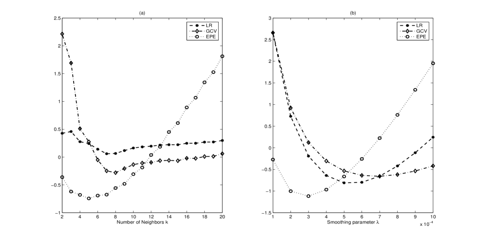
LoRP for selecting a good number of neighbors in kNN. Let us now see how LoRP can be applied to select a good parameter $k$ in kNN regression.

We created a dataset of $n=100$ observations $(x_{i},y_{i})$ from the model:

$$y=f(x)+\varepsilon,\ \mbox{with}\ f(x)={\textstyle{\sin(12(x+0.2))\over x+0.2}},\ x\in[0,1]$$ (19)

where $\varepsilon\sim N(0,\sigma^{2})$ with $\sigma=0.5$. The regression matrix $M^{(k)}$ for kNN regression is determined by $M_{ij}^{(k)}={1\over k}$ if $j\in{\cal N}_{k}(x_{i})$ and 0 else. Then, the loss rank is

$$\text{\rm LR}(k)=\inf_{\alpha\geq 0}\{{\textstyle{n\over 2}}\log(\boldsymbol{y}^{\mskip-3.0mu\top\mskip-3.0mu}S_{\alpha}^{(k)}\boldsymbol{y})-{\textstyle{1\over 2}}\log\det S_{\alpha}^{(k)}\},$$

where $S_{\alpha}^{(k)}=(I-M^{(k)})^{\mskip-3.0mu\top\mskip-3.0mu}(I-M^{(k)})+\alpha I$. The most widely-used method to select a good $k$ is probably Generalized Cross-Validation (GCV) [CW79]: $\text{\rm GCV}(k)=n\|(I-M^{(k)})\boldsymbol{y}\|^{2}/[\text{\rm tr}(I-M^{(k)})]^{2}$. To judge how well GCV and LoRP work, we compare them to the expected prediction error defined as

$$\text{EPE}(k)\mskip 5.0mu plus 5.0mu=\mskip 5.0mu plus 5.0mu\sum_{i=1}^{n}{\bf E}(y_{i}-\hat{y}_{i})^{2}\mskip 5.0mu plus 5.0mu=\mskip 5.0mu plus 5.0mu\sum_{i=1}^{n}\Big{[}\sigma^{2}+(f(x_{i})-{\textstyle{1\over k}}\sum_{j\in{\cal N}_{k}(x_{i})}f(x_{j}))^{2}+{\textstyle{\sigma^{2}\over k}}\Big{]}.$$

Figure 1(a) shows the curves $\text{\rm LR}(k),\ \text{\rm GCV}(k),\ \text{EPE}(k)$ for $k=2,...,20$ (the trivial case $k=1$ is omitted), in which $k=7$-nearest neighbors is chosen by LoRP and $k=8$ is chosen by GCV. The “ideal” $k$ is 5. Both LoRP and GCV do a reasonable job. LoRP works slightly better than GCV.

Refer to caption

Figure 1: Choosing the tuning parameters in kNN and spline regression. The curves have been scaled by their standard deviations.

LoRP for selecting a good smoothing parameter. We now further demonstrate the use of LoRP in selecting a good smoothing parameter for spline regression. Consider the following problem: find a function belonging to the class of functions with continuous 2nd derivative that minimizes the following penalized residual sum of squares:

$$\mbox{RSS}(f)=\sum_{i=1}^{n}(y_{i}-f(x_{i}))^{2}+\lambda\int(f^{\prime\prime}(t))^{2}dt,$$

where $\lambda$ is called the smoothing parameter. The second term penalizes the curvature of function $f$ and the smoothing parameter $\lambda$ controls the amount of penalty. Our goal is to choose a good $\lambda$.

It is well known (see, e.g., [HTF01], Section 5.4) that the solution is a natural spline $f(x)=\sum_{j=1}^{n}N_{j}(x)\theta_{j}$ where $N_{1}(x),...,N_{n}(x)$ are the basis functions of the natural cubic spline:

$$N_{1}(x)=1,\ N_{2}(x)=x,\ N_{k+2}(x)=d_{k}(x)-d_{n-1}(x)\mskip 5.0mu plus 5.0mu\mskip 5.0mu plus 5.0mu\text{with}\mskip 5.0mu plus 5.0mu\mskip 5.0mu plus 5.0mud_{k}(x)={\textstyle{(x-x_{k})_{+}^{3}-(x-x_{n})_{+}^{3}\over x_{n}-x_{k}}}.$$

The problem thus reduces to finding a vector $\boldsymbol{\theta}\in I\mskip-3.0mu\mskip-3.0muR^{n}$ that minimizes

$$\mbox{RSS}(\boldsymbol{\theta})=(\boldsymbol{y}-N\boldsymbol{\theta})^{\mskip-3.0mu\top\mskip-3.0mu}(\boldsymbol{y}-N\boldsymbol{\theta})+\lambda\boldsymbol{\theta}^{\mskip-3.0mu\top\mskip-3.0mu}\Omega\boldsymbol{\theta}$$

where $N_{ij}=N_{j}(x_{i})$ and $\Omega_{ij}=\int N_{i}^{\prime\prime}(x)N_{j}^{\prime\prime}(x)dx$. It is easy to see that the solution is $\boldsymbol{\hat{\theta}}_{\lambda}=(N^{\mskip-3.0mu\top\mskip-3.0mu}N+\lambda\Omega)^{-1}N^{\mskip-3.0mu\top\mskip-3.0mu}\boldsymbol{y}$, and the fitted vector is $\boldsymbol{\hat{y}}=N\boldsymbol{\hat{\theta}}_{\lambda}=M_{\lambda}\boldsymbol{y}$ with $M_{\lambda}=N(N^{\mskip-3.0mu\top\mskip-3.0mu}N+\lambda\Omega)^{-1}N^{\mskip-3.0mu\top\mskip-3.0mu}\boldsymbol{y}$. The fitted vector is linear in $\boldsymbol{y}$, thus the loss rank is

$$\text{\rm LR}(\lambda)=\text{\rm arg}\min_{\alpha\geq 0}\{{\textstyle{n\over 2}}\log(\boldsymbol{y}^{\mskip-3.0mu\top\mskip-3.0mu}S_{\lambda}^{\alpha}\boldsymbol{y})-{\textstyle{1\over 2}}\log\det S_{\lambda}^{\alpha}\}$$

where $S_{\lambda}^{\alpha}=(I-M_{\lambda})^{\mskip-3.0mu\top\mskip-3.0mu}(I-M_{\lambda})+\alpha I$.

Let us consider again the dataset generated from model (19). Figure 1(b) shows the curves $\text{\rm LR}(\lambda)$, $\text{\rm GCV}(\lambda)$ and $\text{EPE}(\lambda)$. The derivation of expressions for $\text{\rm GCV}(\lambda)$ and $\text{EPE}(\lambda)$ is similar to the previous example. $\lambda\approx 3\times 10^{-4}$ is the optimal value selected by the “ideal” criterion EPE. $\lambda\approx 5\times 10^{-4}$ and $\lambda\approx 7\times 10^{-4}$ are selected by LoRP and GCV, respectively. One again, like the previous example, LoRP selects a better $\lambda$ than GCV does.

6 Comparison to Gaussian Bayesian Linear Regression

We now consider LBFR from a Bayesian perspective with Gaussian noise and prior, and compare it to LoRP. In addition to the noise model as in PML, one also has to specify a prior. Bayesian model selection (BMS) proceeds by selecting the model that has largest evidence. In the special case of LBFR with Gaussian noise and prior and a type II maximum likelihood estimate for the noise variance, the expression for the evidence has a similar structure as the expression of the loss rank.

Gaussian Bayesian LBFR / MAP. Recall from Sec.3 Ex.9 that ${\cal F}_{d}$ is the class of functions $f_{\boldsymbol{w}}(x)=\boldsymbol{w}^{\mskip-3.0mu\top\mskip-3.0mu}\boldsymbol{\phi}(x)$ ($\boldsymbol{w}\in I\mskip-3.0mu\mskip-3.0muR^{d}$) that are linear in feature vector $\boldsymbol{\phi}$. Let

$$\text{Gauss}_{N}(\boldsymbol{z}|\boldsymbol{\mu},\sigma)\mskip 5.0mu plus 5.0mu:=\mskip 5.0mu plus 5.0mu{\exp(-{\textstyle{1\over 2}}(\boldsymbol{z}-\boldsymbol{\mu})^{\mskip-3.0mu\top\mskip-3.0mu}\sigma^{-1}(\boldsymbol{z}-\boldsymbol{\mu}))\over(2\pi)^{N/2}\sqrt{\det\sigma}}$$ (20)

denote a general $N$-dimensional Gaussian distribution with mean $\boldsymbol{\mu}$ and covariance matrix $\sigma$. We assume that observations $y$ are perturbed from $f_{\boldsymbol{w}}(x)$ by independent additive Gaussian noise with variance $\beta^{-1}$ and zero mean, i.e., the likelihood of $\boldsymbol{y}$ under model $\boldsymbol{w}$ is ${\rm P}(\boldsymbol{y}|\boldsymbol{w})=\text{Gauss}_{n}(\boldsymbol{y}|\Phi\boldsymbol{w},\beta^{-1}I)$, where $\Phi_{ia}=\boldsymbol{\phi}_{a}(x_{i})$. A Bayesian assumes a prior (before seeing $\boldsymbol{y}$) distribution on $\boldsymbol{w}$. We assume a centered Gaussian with covariance matrix $(\alpha C)^{-1}$, i.e., ${\rm P}(\boldsymbol{w})=\text{Gauss}_{d}(\boldsymbol{w}|\boldsymbol{0},\alpha^{-1}C^{-1})$. From the prior and the likelihood one can compute the evidence and the posterior

$\displaystyle\mbox{Evidence:}\qquad\quad\mskip 5.0mu plus 5.0mu{\rm P}(\boldsymbol{y})$ $\displaystyle=$ $\displaystyle\int{\rm P}(\boldsymbol{y}|\boldsymbol{w}){\rm P}(\boldsymbol{w})d\boldsymbol{w}\mskip 5.0mu plus 5.0mu=\mskip 5.0mu plus 5.0mu\text{Gauss}_{n}(\boldsymbol{y}|\boldsymbol{0},\beta^{-1}S^{-1})$ (21)
$\displaystyle\mbox{Posterior:}\qquad{\rm P}(\boldsymbol{w}|\boldsymbol{y})$ $\displaystyle=$ $\displaystyle{\rm P}(\boldsymbol{y}|\boldsymbol{w}){\rm P}(\boldsymbol{w})/P(\boldsymbol{y})\mskip 5.0mu plus 5.0mu=\mskip 5.0mu plus 5.0mu\text{Gauss}_{d}(\boldsymbol{w}|\boldsymbol{\hat{w}},A^{-1})$
$$B:=\Phi^{\mskip-3.0mu\top\mskip-3.0mu}\Phi,\quad A:=\alpha C+\beta B,\quad M:=\beta\Phi A^{-1}\Phi^{\mskip-3.0mu\top\mskip-3.0mu},\quad S:=I-M,\quad$$ (22)
$$\boldsymbol{\hat{w}}:=\beta A^{-1}\Phi^{\mskip-3.0mu\top\mskip-3.0mu}\boldsymbol{y},\quad\boldsymbol{\hat{y}}:=\Phi\boldsymbol{\hat{w}}=M\boldsymbol{y}$$

A standard Bayesian point estimate for $\boldsymbol{w}$ for fixed $d$ is the one that maximizes the posterior (MAP) (which in the Gaussian case coincides with the mean) $\boldsymbol{\hat{w}}=\text{\rm arg}\max_{\boldsymbol{w}}{\rm P}(\boldsymbol{w}|\boldsymbol{y})=\beta A^{-1}\Phi^{\mskip-3.0mu\top\mskip-3.0mu}\boldsymbol{y}$. For $\alpha\to 0$, MAP reduces to Maximum Likelihood (ML), which in the Gaussian case coincides with the least squares regression of Ex.9. For $\alpha>0$, the regression matrix $M$ is not a projection anymore.

Bayesian model selection. Consider now a family of models $\{{\cal F}_{1},{\cal F}_{2},...\}$. Here the ${\cal F}_{d}$ are the linear regressors with $d$ basis functions, but in general they could be completely different model classes. All quantities in the previous paragraph implicitly depend on the choice of ${\cal F}$, which we now explicate with an index. In particular, the evidence for model class ${\cal F}$ is ${\rm P}_{\cal F}(\boldsymbol{y})$. BMS chooses the model class (here $d$) ${\cal F}$ of highest evidence:

$${\cal F}^{\text{BMS}}\mskip 5.0mu plus 5.0mu=\mskip 5.0mu plus 5.0mu\text{\rm arg}\max_{\cal F}{\rm P}_{\cal F}(\boldsymbol{y})$$

Once the model class ${\cal F}^{\text{BMS}}$ is determined, the MAP (or other) regression function $f_{{\boldsymbol{w}}_{{\cal F}^{\text{BMS}}}}$ or $M_{{\cal F}^{\text{BMS}}}$ are chosen. The data variance $\beta^{-1}$ may be known or estimated from the data, $C$ is often chosen $I$, and $\alpha$ has to be chosen somehow. Note that while $\alpha\to 0$ leads to a reasonable MAP=ML regressor for fixed $d$, this limit cannot be used for BMS.

Comparison to LoRP. Inserting (20) into (21) and taking the logarithm we see that BMS minimizes

$$-\log{\rm P}_{\cal F}(\boldsymbol{y})\mskip 5.0mu plus 5.0mu=\mskip 5.0mu plus 5.0mu{\textstyle{\beta\over 2}}\boldsymbol{y}^{\mskip-3.0mu\top\mskip-3.0mu}S\boldsymbol{y}-{\textstyle{1\over 2}}\log\det S-{\textstyle{n\over 2}}\log{\textstyle{\beta\over 2\pi}}$$ (23)

w.r.t. ${\cal F}$. Let us estimate $\beta$ by ML: We assume a broad prior $\alpha\ll\beta$ so that $\beta{\partial S\over\partial\beta}=O({\alpha\over\beta})$ can be neglected. Then $-{\partial\log{\rm P}_{\cal F}(\boldsymbol{y})\over\partial\beta}={\textstyle{1\over 2}}\boldsymbol{y}^{\mskip-3.0mu\top\mskip-3.0mu}S\boldsymbol{y}-{n\over 2\beta}+O({\alpha\over\beta}n)=0$ $\Leftrightarrow$ $\beta\approx\hat{\beta}:=n/(\boldsymbol{y}^{\mskip-3.0mu\top\mskip-3.0mu}S\boldsymbol{y})$. Inserting $\hat{\beta}$ into (23) we get

$$-\log{\rm P}_{\cal F}(\boldsymbol{y})\mskip 5.0mu plus 5.0mu=\mskip 5.0mu plus 5.0mu{\textstyle{n\over 2}}\log\boldsymbol{y}^{\mskip-3.0mu\top\mskip-3.0mu}S\boldsymbol{y}-{\textstyle{1\over 2}}\log\det S-{\textstyle{n\over 2}}\log{\textstyle{n\over 2\pi{\rm e}}}$$ (24)

Taking an improper prior ${\rm P}(\beta)\propto\beta^{-1}$ and integrating out $\beta$ leads for small $\alpha$ to a similar result. The last term in (24) is a constant independent of ${\cal F}$ and can be ignored. The first two terms have the same structure as in linear LoRP (10), but the matrix $S$ is different. In both cases, $\alpha$ act as regularizers, so we may minimize over $\alpha$ in BMS like in LoRP. For $\alpha=0$ (which neither makes sense in BMS nor in LoRP), $M$ in BMS coincides with $M$ of Ex.9, but still the $S_{0}$ in LoRP is the square of the $S$ in BMS. For $\alpha>0$, $M$ of BMS may be regarded as a regularized regressor as suggested in Sec.2 (a), rather than a regularized loss function (b) used in LoRP. Note also that BMS is limited to (semi)parametric regression, i.e., does not cover the non-parametric kNN Ex.2 and kernel Ex.8, unlike LoRP.

Since $B$ only depends on $\boldsymbol{x}$ (and not on $\boldsymbol{y}$), and all ${\rm P}$ are implicitly conditioned on $\boldsymbol{x}$, one could choose $C=B$. In this case, $M=\gamma\Phi B^{-1}\Phi^{\mskip-3.0mu\top\mskip-3.0mu}$, with $\gamma={\beta\over\alpha+\beta}<1$ for $\alpha>0$, is a simple multiplicative regularization of projection $\Phi B^{-1}\Phi^{\mskip-3.0mu\top\mskip-3.0mu}$, and (24) coincides with (11) for suitable $\alpha$, apart from an irrelevant additive constant, hence minimizing (24) over $\alpha$ also leads to (12).

7 Comparison to other Model Selection Schemes

In this section we give a brief introduction to PML for (semi)parametric regression, and its major instantiations, AIC, BIC, and MDL principle, whose penalty terms are all proportional to the number of parameters $d$. The effective number of parameters is often much smaller than $d$, e.g., if there are soft constraints like in ridge regression. We compare MacKay’s trace formula [Mac92] for Gaussian Bayesian LBFR and Hastie’s et al. trace formula [HTF01] for general linear regression with LoRP.

Penalized ML (AIC, BIC, MDL). Consider a $d$-dimensional stochastic model class like the Gaussian Bayesian linear regression example of Section 6. Let ${\rm P}_{d}(\boldsymbol{y}|\boldsymbol{w})$ be the data likelihood under $d$-dimensional model $\boldsymbol{w}\in I\mskip-3.0mu\mskip-3.0muR^{d}$. The maximum likelihood (ML) estimator for fixed $d$ is

$$\boldsymbol{\hat{w}}\mskip 5.0mu plus 5.0mu=\mskip 5.0mu plus 5.0mu\text{\rm arg}\max_{\boldsymbol{w}}{\rm P}_{d}(\boldsymbol{y}|\boldsymbol{w})\mskip 5.0mu plus 5.0mu=\mskip 5.0mu plus 5.0mu\text{\rm arg}\min_{\boldsymbol{w}}\{-\log{\rm P}_{d}(\boldsymbol{y}|\boldsymbol{w})\}$$ (25)

Since $-\log{\rm P}_{d}(\boldsymbol{y}|\boldsymbol{w})$ decreases with $d$, we cannot find the model dimension by simply minimizing over $d$ (overfitting). Penalized ML adds a complexity term to get reasonable results

$$\hat{d}\mskip 5.0mu plus 5.0mu=\mskip 5.0mu plus 5.0mu\text{\rm arg}\min_{d}\{-\log{\rm P}_{d}(\boldsymbol{y}|\boldsymbol{\hat{w}})+\mbox{Penalty}(d)\}$$ (26)

The penalty introduces a tradeoff between the first and second term with a minimum at $\hat{d}<\infty$. Various penalties have been suggested: AIC [Aka73] uses $d$, BIC [Sch78] and the (crude) MDL [Ris78, Grü04] use ${\textstyle{d\over 2}}\log n$ for Penalty$(d)$. There are at least three important conceptual differences to LoRP:

  • In order to apply PML one needs to specify not only a class of regression functions, but a full probabilistic model ${\rm P}_{d}(\boldsymbol{y}|\boldsymbol{w})$,

  • PML ignores or at least does not tell how to incorporate a potentially given loss-function,

  • PML is mostly limited to selecting between (semi)parametric models.

We discuss two approaches to the last item in the remainder of this section (where AIC, BIC, and MDL are not directly applicable): (a) for non-parametric models like kNN or kernel regression, or (b) if $d$ does not reflect the “true” complexity of the model. [Mac92] suggests an expression for the effective number of parameters $d_{e\mskip-3.0muf\mskip-3.0muf}$ as a substitute for $d$ in case of (b), while [HTF01] introduce another expression which is applicable for both (a) and (b).

The trace penalty for parametric Gaussian LBFR. We continue with the Gaussian Bayesian linear regression example (see Section 6 for details and notation). Performing the integration in (21), [Mac92, Eq.(21)] derives the following expression for the Bayesian evidence for $C=I$

$\displaystyle-\log{\rm P}(\boldsymbol{y})$ $\displaystyle=$ $\displaystyle(\alpha\hat{E}_{W}+\beta\hat{E}_{D})+({\textstyle{1\over 2}}\log\det A-{\textstyle{d\over 2}}\log\alpha)-{\textstyle{n\over 2}}\log{\textstyle{\beta\over 2\pi}}$ (27)
$\displaystyle\hat{E}_{D}$ $\displaystyle=$ $\displaystyle{\textstyle{1\over 2}}\|\Phi\boldsymbol{\hat{w}}-\boldsymbol{y}\|_{2}^{2},\quad\hat{E}_{W}={\textstyle{1\over 2}}\|\boldsymbol{\hat{w}}\|_{2}^{2}$

(the first bracket in (27) equals ${\textstyle{\beta\over 2}}\boldsymbol{y}^{\mskip-3.0mu\top\mskip-3.0mu}S\boldsymbol{y}$ and the second equals $-{\textstyle{1\over 2}}\log\det S$, cf. (23)). Minimizing (27) w.r.t. $\alpha$ leads to the following relation:

$$0\mskip 5.0mu plus 5.0mu=\mskip 5.0mu plus 5.0mu\textstyle{-\partial\log{\rm P}(\boldsymbol{y})\over\partial\alpha}\mskip 5.0mu plus 5.0mu=\mskip 5.0mu plus 5.0mu\hat{E}_{W}+{\textstyle{1\over 2}}\text{\rm tr}A^{-1}-{\textstyle{d\over 2\alpha}}\qquad({\partial\over\partial\alpha}\log\det A=\text{\rm tr}A^{-1})$$

He argues that $\alpha\|\boldsymbol{\hat{w}}\|_{2}^{2}$ corresponds to the effective number of parameters, hence

$$d^{\text{McK}}_{e\mskip-3.0muf\mskip-3.0muf}\mskip 5.0mu plus 5.0mu:=\mskip 5.0mu plus 5.0mu\alpha\|\boldsymbol{\hat{w}}\|_{2}^{2}\mskip 5.0mu plus 5.0mu=\mskip 5.0mu plus 5.0mu2\alpha\hat{E}_{W}\mskip 5.0mu plus 5.0mu=\mskip 5.0mu plus 5.0mud-\alpha\text{\rm tr}A^{-1}$$ (28)

The trace penalty for general linear models. We now return to general linear regression $\boldsymbol{\hat{y}}=M(\boldsymbol{x})\boldsymbol{y}$ (7). LBFR is a special case of a projection matrix $M=M^{2}$ with rank $d=\text{\rm tr}M$ being the number of basis functions. $M$ leaves $d$ directions untouched and projects all other $n-d$ directions to zero. For general $M$, [HTF01, Sec.5.4.1] argue to regard a direction that is only somewhat shrunken, say by a factor of $0<\beta<1$, as a fractional parameter ($\beta$ degrees of freedom). If $\beta_{1},...,\beta_{n}$ are the shrinkages = eigenvalues of $M$, the effective number of parameters could be defined as [HTF01, Sec.7.6]

$$d^{\text{HTF}}_{e\mskip-3.0muf\mskip-3.0muf}\mskip 5.0mu plus 5.0mu:=\mskip 5.0mu plus 5.0mu\sum_{i=1}^{n}\beta_{i}\mskip 5.0mu plus 5.0mu=\mskip 5.0mu plus 5.0mu\text{\rm tr}M,$$

where HTF stands for Hastie-Tibshirani-Friedman, which generalizes the relation $d=\text{\rm tr}M$ beyond projections. For MacKay’s $M$ (22), $\text{\rm tr}M=d-\alpha\text{\rm tr}A^{-1}$, i.e., $d^{\text{HTF}}_{e\mskip-3.0muf\mskip-3.0muf}$ is consistent with and generalizes $d^{\text{McK}}_{e\mskip-3.0muf\mskip-3.0muf}$.

Problems. Though nicely motivated, the trace formula is not without problems. First, since for projections, $M=M^{2}$, one could have argued equally well for $d^{\text{HTF}}_{e\mskip-3.0muf\mskip-3.0muf}=\text{\rm tr}M^{2}$. Second, for kNN we have $\text{\rm tr}M={\textstyle{n\over k}}$ (since $M$ is ${\textstyle{1\over k}}$ on the diagonal), which does not look unreasonable. Consider now kNN’, which is defined as follows: we average over the $k$ nearest neighbors excluding the closest neighbor. For sufficiently smooth functions, kNN’ for suitable $k$ is still a reasonable regressor, but $\text{\rm tr}M=0$ (since $M$ is zero on the diagonal). So $d^{\text{HTF}}_{e\mskip-3.0muf\mskip-3.0muf}=0$ for kNN’, which makes no sense and would lead one to always select the $k=1$ model.

Relation to LoRP. In the case of kNN’, $\text{\rm tr}M^{2}$ would be a better estimate for the effective dimension. In linear LoRP, $-\log\det S_{\alpha}$ serves as complexity penalty. Ignoring the nullspace of $S_{0}=(I-M)^{\mskip-3.0mu\top\mskip-3.0mu}(I-M)$ (8), we can Taylor expand $-{\textstyle{1\over 2}}\log\det S_{0}$ in $M$

$$-{\textstyle{1\over 2}}\log\det S_{0}\mskip 5.0mu plus 5.0mu=\mskip 5.0mu plus 5.0mu-\text{\rm tr}\log(I\mskip-3.0mu-\mskip-3.0muM)\mskip 5.0mu plus 5.0mu=\mskip 5.0mu plus 5.0mu\sum_{s=1}^{\infty}{\textstyle{1\over s}}\text{\rm tr}(M^{s})\mskip 5.0mu plus 5.0mu=\mskip 5.0mu plus 5.0mu\text{\rm tr}M+{\textstyle{1\over 2}}\text{\rm tr}M^{2}+...$$

For BMS (24) with $S=I-M$ (22) we get half of this value. So the trace penalty may be regarded as a leading order approximation to LoRP. The higher order terms prevent peculiarities like in kNN’.

Coding/MDL interpretation of LoRP. The basic idea of MDL is as follows [Grü04]: “The goal of statistical inferences may be cast as trying to find regularity in the data. ‘Regularity’ may be identified with ‘ability to compress’. MDL combines these two insights by viewing learning as data compression: it tells us that, for a given set of hypotheses $\cal H$ and data set $D$, we should try to find the hypothesis or combination of hypotheses in $\cal H$ that compress $D$ most.”

The standard incarnation of (crude) MDL is as follows: If $H$ is a stochastic model of (discrete) data $D$, we can code $D$ (by Shannon-Fano) in $\lceil-{\log_{2}}{\rm P}(D|H)\rceil$ bits. If we have a class of models $\cal H$, we also have to code $H$ (somehow in, say, $L(H)$ bits) in order to be able to decode $D$. MDL chooses the hypothesis $H^{\text{\rm MDL}}=\text{\rm arg}\min_{H\in\cal H}\{-{\log_{2}}{\rm P}(D|H)+L(H)\}$ of minimal two-part code. For instance, if $\cal H$ is the class of all polynomials of all degrees with each coefficient coded to ${\textstyle{1\over 2}}{\log_{2}}n$ bits (i.e., $O(n^{-1/2})$ accuracy) and we condition on $x$, i.e., $D\leadsto\boldsymbol{y}|\boldsymbol{x}$, MDL takes the form (25) and (26), i.e., $H^{\text{\rm MDL}}=(\boldsymbol{\hat{w}},\hat{d})$.

We now give LoRP (for discrete $D$) a data compression/MDL interpretation. For simplicity, we will first assume that all loss values are different, i.e., if $\text{\rm Loss}_{r}(\boldsymbol{y}^{\prime}|\boldsymbol{x})\neq\text{\rm Loss}_{r}(\boldsymbol{y}^{\prime\prime}|\boldsymbol{x})$ for $\boldsymbol{y}^{\prime}\neq\boldsymbol{y}^{\prime\prime}$ (adding infinitesimal random noise to $\text{\rm Loss}_{r}$ easily ensures this). In this case, $\text{\rm Rank}_{r}(\cdot|\boldsymbol{x}):{\cal Y}^{n}\to I\mskip-3.0mu\mskip-3.0muN$ is an order preserving bijection, i.e., $\text{\rm Rank}_{r}(\boldsymbol{y}^{\prime}|\boldsymbol{x})<\text{\rm Rank}_{r}(\boldsymbol{y}^{\prime\prime}|\boldsymbol{x})$ iff $\text{\rm Loss}_{r}(\boldsymbol{y}^{\prime}|\boldsymbol{x})<\text{\rm Loss}_{r}(\boldsymbol{y}^{\prime\prime}|\boldsymbol{x})$ with no gaps in the range of $\text{\rm Rank}_{r}(\cdot|\boldsymbol{x})$.

Phrased differently, $\text{\rm Rank}_{r}(\cdot|\boldsymbol{x})$ codes each $\boldsymbol{y}^{\prime}\in{\cal Y}^{n}$ as a natural number $m$ in increasing loss-order. The natural number $m$ can itself be coded in $\lceil{\log_{2}}m\rceil$ bits (using plain not prefix coding). Let us call this code of $\boldsymbol{y}^{\prime}$ the Loss Rank Code (LRC). LRC has a nice characterization: LRC is the shortest loss-order preserving code. Ignoring the rounding, the Length of LRC${}_{r}(\boldsymbol{y}^{\prime}|\boldsymbol{x})$ is $\text{\rm LR}_{r}(\boldsymbol{y}^{\prime}|\boldsymbol{x})$:

Proposition 15 (Minimality property)

If all loss values are different, i.e., if

$$\text{\rm Loss}_{r}(\boldsymbol{y}^{\prime}|\boldsymbol{x})\neq\text{\rm Loss}_{r}(\boldsymbol{y}^{\prime\prime}|\boldsymbol{x})\mbox{ for all }\boldsymbol{y}^{\prime}\neq\boldsymbol{y}^{\prime\prime}$$

then the loss rank (code) of $\boldsymbol{y}$ is the smallest/shortest among all loss-order preserving rankings/codes $C$ in the sense that

$\displaystyle\text{\rm Rank}(\boldsymbol{y})$ $\displaystyle=$ $\displaystyle\min\{C(\boldsymbol{y})\mskip 3.0mu:\mskip 3.0muC\in{\cal Y}^{n}\mskip-3.0mu\to\mskip-3.0muI\mskip-3.0mu\mskip-3.0muN\mskip 3.0mu\wedge\mskip 3.0mu(\star)\mskip 3.0mu\}$
$\displaystyle\lfloor\text{\rm LR}(\boldsymbol{y})/\log 2\rfloor$ $\displaystyle=$ $\displaystyle\min\{\text{\rm Length}(C(\boldsymbol{y}))\mskip 3.0mu:\mskip 3.0muC\in{\cal Y}^{n}\mskip-3.0mu\to\mskip-3.0mu\{0,1\}^{*}\mskip 3.0mu\wedge\mskip 3.0mu(\star)\mskip 3.0mu\}$
$\displaystyle(\star)$ $\displaystyle:=$ $\displaystyle[\text{\rm Loss}(\boldsymbol{y}^{\prime})<\text{\rm Loss}(\boldsymbol{y}^{\prime\prime})\Leftrightarrow C(\boldsymbol{y}^{\prime})<C(\boldsymbol{y}^{\prime\prime}),\mskip 3.0mu\forall\boldsymbol{y}^{\prime},\boldsymbol{y}^{\prime\prime}]$

The proof follows from the fact that if a discrete injection (code) is order preserving, there exists a “smallest” one without gaps in the range. So LoRP minimizes the Loss Rank Code, where LRC itself is the shortest among all loss-order preserving codes. From this perspective, LoRP is just a different (non-stochastic, non-parametric, loss-based) incarnation of MDL. The MDL philosophy provides a justification of LoRP (2), its regularization (5), and loss function selection (Section 8). This identification should also allow to apply or adapt the various consistency results of MDL, implying that LoRP is consistent under some mild conditions.

If some losses are equal, $\text{\rm Rank}_{r}(\cdot|\boldsymbol{x}):{\cal Y}^{n}\to I\mskip-3.0mu\mskip-3.0muN$ still preserves the order $\leq$, but the mapping is neither surjective nor injective anymore.

Large regression classes ${\cal R}$. The classes ${\cal R}$ of regressors we considered so far were discrete and “small”, often indexed by an integer complexity index (like $k$ in kNN or $d$ in LBFR). But large classes are also thinkable.

As an extreme case, consider the class of all regressors. Clearly, there is an $r=r_{D}$ which “knows” $D$ and perfectly fits $D$ ($r(x_{i}|D)=y_{i},\ \forall i$), but is the worst possible on all other $D^{\prime}$ ($r(x_{i}|D^{\prime})=\infty,\ \forall i,\ \forall D^{\prime}\neq D$). This $r$ has (discrete) Rank 1, so is best according to LoRP. So if ${\cal R}$ is too large, LoRP can overfit too.

Consider a more realistic example by not taking all of the first $d$ basis functions in LBFR, but selecting some basis functions $\phi_{i_{1}},...,\phi_{i_{d}}$, i.e., ${\cal R}$ is indexed by $d$ integers, and $d$ may be variable too.

One solution approach is to group more regressors in ${\cal R}$ into one function class ${\cal F}$, e.g., the class of functions ${\cal F}_{k,d}=\{w_{1}\phi_{i_{1}}+...w_{d}\phi_{i_{d}}:\boldsymbol{w}\in I\mskip-3.0mu\mskip-3.0muR^{d},\mskip 3.0mu1\leq i_{1}<...<i_{d}\leq k\}$ that are linear in $d$ of the first $k$ bases. Now ${\cal R}$ is a small class indexed by $d$ and $k$ only.

Looking at the coding interpretation of $\text{\rm LR}_{r}$ and the MDL philosophy, suggests to assign a code to $r\in I\mskip-3.0mu\mskip-3.0muR$ in order to get a complete code for $D$:

$$r^{best}\mskip 5.0mu plus 5.0mu=\mskip 5.0mu plus 5.0mu\text{\rm arg}\min_{r}\{\text{\rm LR}_{r}(\boldsymbol{y}|\boldsymbol{x})+L(r)\}$$

where $r$ is the length of a code for $r$ (given ${\cal R}$). For ${\cal R}\simeq I\mskip-3.0mu\mskip-3.0muN$ a single integer has to be coded, e.g., $k$ in $L(r)=L(k)\approx{\log_{2}}k$ bits, which can usually be safely dropped/ignored. For more complex classes like the (ungrouped) LBFR subset selection above, $L(r)=L(i_{1},...,i_{d},d)\approx d{\log_{2}}k+{\log_{2}}d$ can become important.

8 Loss Functions and their Selection

General additive loss. Linear LoRP $\boldsymbol{\hat{y}}=M(\boldsymbol{x})\boldsymbol{y}$ of Section 3 can easily be generalized to non-quadratic loss. Let us consider the $\rho>0$ loss

$\displaystyle\text{\rm Loss}_{M}(\boldsymbol{y}|\boldsymbol{x})$ $\displaystyle:=$ $\displaystyle\textstyle(\sum_{i=1}^{n}(y_{i}-\hat{y}_{i})^{\rho})^{{}^{1}\mskip-3.0mu/\mskip-3.0mu_{\rho}}\mskip 5.0mu plus 5.0mu=\mskip 5.0mu plus 5.0mu\|\boldsymbol{y}-\boldsymbol{\hat{y}}\|_{\rho}\mskip 5.0mu plus 5.0mu=\mskip 5.0mu plus 5.0mu\|(I\mskip-3.0mu-\mskip-3.0muM)\boldsymbol{y}\|_{\rho}$
$\displaystyle V(L)$ $\displaystyle=$ $\displaystyle\{\boldsymbol{y}^{\prime}\in I\mskip-3.0mu\mskip-3.0muR^{n}:\|(I\mskip-3.0mu-\mskip-3.0muM)\boldsymbol{y}^{\prime}\|_{\rho}\leq L\}\mskip 5.0mu plus 5.0mu=\mskip 5.0mu plus 5.0mu\{(I\mskip-3.0mu-\mskip-3.0muM)^{-1}\boldsymbol{z}\in I\mskip-3.0mu\mskip-3.0muR^{n}:\|\boldsymbol{z}\|_{\rho}\leq L\}$
$\displaystyle\mbox{Let}\quad v_{n}^{\rho}$ $\displaystyle:=$ $\displaystyle|\{\boldsymbol{z}\in I\mskip-3.0mu\mskip-3.0muR^{n}:\|\boldsymbol{z}\|_{\rho}\leq 1\}|\mskip 5.0mu plus 5.0mu=\mskip 5.0mu plus 5.0mu\textstyle 2^{n}\prod_{i=1}^{n-1}{i\over\rho}!{1\over\rho}!/{i+1\over\rho}!,$

where $\frac{i}{\rho}!:=\Gamma(\frac{i}{\rho}+1)$, be the volume of the unit $d$-dimensional $\rho$-norm “ball”. Since $V(L)$ is a linear transformation of this ball with transformation matrix $(I-M)^{-1}$ and scaling $L$, we have $|V(L)|=v_{n}^{\rho}L^{n}/\det(I-M)$, hence

$$\text{\rm LR}_{M}(\boldsymbol{y}|\boldsymbol{x})\mskip 5.0mu plus 5.0mu=\mskip 5.0mu plus 5.0mu\log|V(\text{\rm Loss}_{M}(\boldsymbol{y}|\boldsymbol{x}))|\mskip 5.0mu plus 5.0mu=\mskip 5.0mu plus 5.0mun\log\|(I\mskip-3.0mu-\mskip-3.0muM)\boldsymbol{y}\|_{\rho}-\log\det(I\mskip-3.0mu-\mskip-3.0muM)+\log v_{n}^{\rho}$$ (29)

For the $\rho=2$ norm, (29) reduces to $\text{\rm LR}_{M}^{0}$ (9). Note that $\text{\rm Loss}_{M}:=g(\|\boldsymbol{y}-\boldsymbol{\hat{y}}\|_{\rho})$ leads to the same result (29) for any monotone increasing $g$, i.e., only the order of the loss matters, not its absolute value. More generally $\text{\rm Loss}_{M}=g(\sum_{i}h(y_{i}-\hat{y}_{i}))$ for any $h$ implies

$\displaystyle\text{\rm LR}_{M}(\boldsymbol{y}|\boldsymbol{x})$ $\displaystyle=$ $\displaystyle\textstyle n\log v_{n}^{h}(\sum_{i}h(y_{i}-\hat{y}_{i}))-\log\det(I\mskip-3.0mu-\mskip-3.0muM),{\quad\mbox{where}\quad}$
$\displaystyle v_{n}^{h}(l)$ $\displaystyle:=$ $\displaystyle\textstyle|\{\boldsymbol{z}\in I\mskip-3.0mu\mskip-3.0muR^{n}:\sum_{i}h(z_{i})\leq l\}|^{{{}^{1}\mskip-3.0mu/\mskip-3.0mu_{n}}}$

is a one-dimensional function of $l$ (independent $D$ and $M$), once to be determined (e.g., $v_{n}^{h}(l)=l\cdot(v_{n}^{\rho})^{{{}^{1}\mskip-3.0mu/\mskip-3.0mu_{n}}}\propto l$ for $\rho$-norm loss). Regularization may be performed by $M\leadsto\gamma M$ with optimization over $\gamma<1$.

Loss-function selection. In principle, the loss function should be part of the problem specification, since it characterizes the ultimate goal. For instance, whether a test should more likely classify a healthy person as sick than a sick person as healthy, depends on the severity of a misclassification (loss) in each direction. In reality, though, having to specify the loss function can be a nuisance. Sure, the loss has to respect some general features, e.g., that it increases with the deviation of $\hat{y}_{i}$ from $y_{i}$. Otherwise it is chosen by convenience or rules of thumb, rather than by elicitation of the real goal, for instance preferring the Euclidean norm over $\rho\neq 2$ norms. If we subscribe to the procedure of choosing the loss function, we could ask whether this may be done in a more principled way. Consider a (not too large) class of loss functions $\text{\rm Loss}^{\alpha}$, indexed by some parameter $\alpha$. For instance, $\text{\rm Loss}^{\alpha}=\|\boldsymbol{y}-\boldsymbol{\hat{y}}\|_{\alpha}$ from the previous paragraph. The regularized loss (5) also constitutes a class of losses. In this case we minimized over the regularization parameter $\alpha$. This suggests to choose in general the loss function that has minimal loss rank $\text{\rm LR}_{r}^{\alpha}$. The justifications are similar to the ones for minimizing $\text{\rm LR}_{r}^{\alpha}$ w.r.t. $r$. Note that the term $\log v_{n}^{\rho}$ cannot be dropped anymore, unlike in (10).

9 Self-Consistent Regression

So far we have considered only “on-data” regression. LoRP only depends on the regressor $r$ on data $D$ and not on $x\not\in\{x_{1},...,x_{n}\}$. We now construct canonical regressors for off-data $x$ from regressors given only on-data. First, this may ease the specification of the regression functions, second, it is a canonical way for interpolation (LoRP can’t distinguish between $r$ that are identical on $D$), and third, we show that many standard regressors (kNN, Kernel, LBFR) are self-consistent in the sense that they are canonical. We limit our exposition to linear regression.

Off-data regression. A linear regressor is completely determined by the $n$ functions $m_{j}$ (6), but not by the matrix function $M$ (7). Indeed, two sets $\{m_{j}\}$ and $\{m^{\prime}_{j}\}$ that coincide on $D=(\boldsymbol{x},\boldsymbol{y})$, i.e. $m_{j}(x_{i}|\boldsymbol{x})=m^{\prime}_{j}(x_{i}|\boldsymbol{x})\mskip 3.0mu\forall i,j$ but possibly differ for $x\not\in\boldsymbol{x}$, lead to the same matrix $M_{ij}(\boldsymbol{x})=m_{j}(x_{i}|\boldsymbol{x})=m^{\prime}_{j}(x_{i}|\boldsymbol{x})$. LoRP has the advantage of only depending on $M$, but this also means that it cannot distinguish between an $m_{j}$ that behaves well on $x\not\in\boldsymbol{x}$ and one that, e.g., wildly oscillates outside $\boldsymbol{x}$.

Typically, the $m_{j}$ are given and, provided the model complexity is chosen appropriately e.g. by LoRP, they properly interpolate $\boldsymbol{x}$. Nevertheless, a canonical extension from $M$ to $m_{j}$ would be nice. In this way LoRP would not be vulnerable to bad $m_{j}$, and we could interpolate $D$ (predict $y$ for any $x\in{\cal X}$) even without $m_{j}$ given a-priori.

We define a self-consistent regression scheme based only on $M$ (for all $n$). We ask for an estimate $\hat{y}$ of $y$ for $x\not\in\boldsymbol{x}$. We add a virtual data point $(x_{0},y_{0})$ to $D$, where $x_{0}=x$. If we knew $y_{0}=y$ we could estimate $\hat{y}_{0}=r(x_{0}|\{(x_{0},y_{0})\}\cup D)$, but we don’t know $y_{0}$. But we could require a self-consistency condition, namely that $\hat{y}_{0}=y_{0}$ for $x_{0}\not\in\boldsymbol{x}$.

Definition 16 (canonical and self-consistent regressors)

Let $M^{\prime}_{ij}(\boldsymbol{x}^{\prime})_{0\leq i,j\leq n}$ be the regression matrix for the data set $D^{\prime}=\{(x_{0},y_{0})\}\cup D=((x_{0},\boldsymbol{x}),(y_{0},\boldsymbol{y}))=(\boldsymbol{x}^{\prime},\boldsymbol{y}^{\prime})$ of size $n+1$.

  • (i)

    A linear regressor $\tilde{y}_{0}=\tilde{r}(x_{0}|D)$ is called a canonical regressor for $M^{\prime}$ if the consistency condition $\tilde{y}_{0}=r(x_{0}|D^{\prime})\equiv\sum_{j=0}^{n}M^{\prime}_{0j}y_{j}$ holds $\forall x_{0},D$.

  • (ii)

    A regressor $r$ is called self-consistent if $\tilde{r}=r$, i.e. if
    $r(x_{0}|\{(x_{0},r(x_{0}|D))\}\cup D)=r(x_{0}|D)$ $\forall x_{0},D$.

  • (iii)

    A class of regressors ${\cal R}=\{r\}$ is called self-consistent if $\tilde{R}=\{\tilde{r}\}\subseteq{\cal R}$.

We denote the solution of the self-consistency condition $y_{0}=\sum_{j=0}^{n}M^{\prime}_{0j}y_{j}$ by $\tilde{y}_{0}$. So we have to solve

$$\tilde{y}_{0}\mskip 5.0mu plus 5.0mu=\mskip 5.0mu plus 5.0mu\sum_{j=1}^{n}M^{\prime}_{0j}y_{j}+M^{\prime}_{00}\tilde{y}_{0}\quad\Longrightarrow\quad\tilde{y}_{0}\mskip 5.0mu plus 5.0mu=\mskip 5.0mu plus 5.0mu{\sum_{j=1}^{n}M^{\prime}_{0j}y_{j}\over 1-M^{\prime}_{00}}\mskip 5.0mu plus 5.0mu=\mskip 5.0mu plus 5.0mu{\sum_{j=1}^{n}M^{\prime}_{0j}y_{j}\over\sum_{j=1}^{n}M^{\prime}_{0j}}$$

where the last equality only holds if $\sum_{j=0}^{n}M^{\prime}_{0j}=1$, which is often the case, in particular for kNN and Kernel regression, but not necessarily for LBFR.

Proposition 17 (canonical regressor)

The linear regressor

$$y_{0}\mskip 5.0mu plus 5.0mu=\mskip 5.0mu plus 5.0mu\tilde{r}(x_{0}|D)\mskip 5.0mu plus 5.0mu:=\mskip 5.0mu plus 5.0mu\sum_{j=1}^{n}\tilde{m}_{j}(x_{0}|\boldsymbol{x})y_{j},{\quad\mbox{where}\quad}\tilde{m}_{j}(x_{0}|\boldsymbol{x}):={M^{\prime}_{0j}(\boldsymbol{x}^{\prime})\over 1-M^{\prime}_{00}(\boldsymbol{x}^{\prime})}$$

is the unique canonical regressor for $M^{\prime}$ (if $M^{\prime}_{00}<1$).

Example 18 (self-consistent kNN, $\uparrow$Ex.2)

$M^{\prime}_{0j}(\boldsymbol{x}^{\prime})={\textstyle{1\over k}}$ for $x_{j}\in{\cal N}^{\prime}_{k}(x_{0})$ and 0 else. The $k$ nearest neighbors ${\cal N}^{\prime}_{k}(x_{0})$ of $x_{0}$ among $\boldsymbol{x}^{\prime}$ consist of $x_{0}$ and the $k-1$ nearest neighbors ${\cal N}_{k-1}(x_{0})=:J$ of $x_{0}$ among $\boldsymbol{x}$, i.e. ${\cal N}^{\prime}_{k}(x_{0})=\{x_{0}\}\cup{\cal N}_{k-1}(x_{0})$. Hence

$$\tilde{y}_{0}\mskip 5.0mu plus 5.0mu=\mskip 5.0mu plus 5.0mu{\sum_{j=1}^{n}M^{\prime}_{0j}y_{j}\over\sum_{j=1}^{n}M^{\prime}_{0j}}\mskip 5.0mu plus 5.0mu=\mskip 5.0mu plus 5.0mu{\sum_{j\in J}{\textstyle{1\over k}}y_{j}\over\sum_{j\in J}{\textstyle{1\over k}}}\mskip 5.0mu plus 5.0mu=\mskip 5.0mu plus 5.0mu\sum_{j\in J}{\textstyle{1\over k-1}}y_{j}\mskip 5.0mu plus 5.0mu=\mskip 5.0mu plus 5.0mu\sum_{j=1}^{n}M_{0j}^{(k-1)}y_{j}\mskip 5.0mu plus 5.0mu=\mskip 5.0mu plus 5.0mur_{k-1}(x_{0}|D)=\hat{y}_{0}$$

Canonical kNN is equivalent to standard (k–1)NN, so the class of canonical kNN regressors coincides with the standard kNN class. $\diamondsuit\quad$

Example 19 (self-consistent kernel)
$$M^{\prime}_{0j}(\boldsymbol{x}^{\prime})\mskip 5.0mu plus 5.0mu=\mskip 5.0mu plus 5.0mu{K(x_{0},x_{j})\over\sum_{j=0}^{n}K(x_{0},x_{j})}\quad\Longrightarrow\quad\tilde{y}_{0}\mskip 5.0mu plus 5.0mu=\mskip 5.0mu plus 5.0mu{\sum_{j=1}^{n}K(x_{0},x_{j})y_{j}\over\sum_{j=1}^{n}K(x_{0},x_{j})}\mskip 5.0mu plus 5.0mu=\mskip 5.0mu plus 5.0mur(x_{0}|D)\mskip 5.0mu plus 5.0mu=\mskip 5.0mu plus 5.0mu\hat{y}_{0}$$

Canonical kernel regression coincides with the standard kernel smoother. $\diamondsuit\quad$

Example 20 (self-consistent LBFR)
$\displaystyle B^{\prime}$ $\displaystyle=$ $\displaystyle\sum_{i=0}^{n}\boldsymbol{\phi}(x_{i})\boldsymbol{\phi}(x_{i})^{\mskip-3.0mu\top\mskip-3.0mu}=B+\boldsymbol{\phi}(x_{0})\boldsymbol{\phi}(x_{0})^{\mskip-3.0mu\top\mskip-3.0mu}$
$\displaystyle\Rightarrow\quad M^{\prime}_{0j}$ $\displaystyle=$ $\displaystyle\boldsymbol{\phi}(x_{0})^{\mskip-3.0mu\top\mskip-3.0mu}B^{\prime}\mskip-3.0mu\mskip 3.0mu{}^{-1}\boldsymbol{\phi}(x_{j})\mskip 5.0mu plus 5.0mu=\mskip 5.0mu plus 5.0mu\boldsymbol{\phi}(x_{0})^{\mskip-3.0mu\top\mskip-3.0mu}\bigg{[}B^{-1}-{B^{-1}\boldsymbol{\phi}(x_{0})\boldsymbol{\phi}(x_{0})^{\mskip-3.0mu\top\mskip-3.0mu}B^{-1}\over 1+\boldsymbol{\phi}(x_{0})^{\mskip-3.0mu\top\mskip-3.0mu}B^{-1}\boldsymbol{\phi}(x_{0})}\bigg{]}\boldsymbol{\phi}(x_{j})$
$\displaystyle=$ $\displaystyle M_{0j}-{M_{00}M_{0j}\over 1+M_{00}}\mskip 5.0mu plus 5.0mu=\mskip 5.0mu plus 5.0mu{M_{0j}\over 1+M_{00}}\quad\Rightarrow\quad 1-M^{\prime}_{00}={1\over 1+M_{00}}$

In the first line we used the Sherman-Morrison formula for inverting $B^{\prime}$. In the second line we defined $M_{0j}=\boldsymbol{\phi}(x_{0})^{\mskip-3.0mu\top\mskip-3.0mu}B^{-1}\boldsymbol{\phi}(x_{j})$, extending $M$.

$$\Rightarrow\quad\tilde{y}_{0}\mskip 5.0mu plus 5.0mu=\mskip 5.0mu plus 5.0mu{\sum_{j=1}^{n}M^{\prime}_{0j}y_{j}\over 1-M^{\prime}_{00}}\mskip 5.0mu plus 5.0mu=\mskip 5.0mu plus 5.0mu\sum_{j=1}^{n}M_{0j}y_{j}\mskip 5.0mu plus 5.0mu=\mskip 5.0mu plus 5.0mu\sum_{j=1}^{n}m_{j}(x_{0},\boldsymbol{x})y_{j}\mskip 5.0mu plus 5.0mu=\mskip 5.0mu plus 5.0mu\hat{y}_{0}$$

Canonical LBFR coincides with standard LBFR. $\diamondsuit\quad$

Proposition 21 (self-consistent regressors)

Kernel regression and linear basis function regression are self-consistent. kNN is not self-consistent but the class of kNN regressors ${\cal R}=\{r_{\text{kNN}}:k\in I\mskip-3.0mu\mskip-3.0muN\}$ is self-consistent.

To summarize, we expect LoRP to select good regressors with proper interpolation behavior for canonical and self-consistent regressors.

10 Nearest Neighbors Classification

We now consider k-nearest neighbors classification in more detail. In order to get more insight into LoRP we seek a case that allows analytic solution. In general, the determinant $\det S_{\alpha}$ cannot be computed analytically, but for $\boldsymbol{x}$ lying on a hypercube of the regular grid ${\cal X}=Z\mskip-3.0mu\mskip-3.0mu\mskip-3.0muZ^{d}$ we can. We derive exact expressions, and consider the limits $n\to\infty$, $k\to\infty$, and $d\to\infty$.

kNN on one-dimensional grid. We consider the $d=1$ dimensional case first. We assume $\boldsymbol{x}=(1,2,3,...,n)$, a circular metric $d(x_{i},x_{j})=d(i,j)=\min\{|i-j|,n-|i-j|\}$, and odd $k\leq n$. The kNN regression matrix

$$M_{ij}=b_{i-j}{\quad\mbox{with}\quad}b_{i-j}={\textstyle{1\over k}}{\quad\mbox{if}\quad}d(i,j)\leq{\textstyle{k-1\over 2}}{\quad\mbox{and}\quad}0{\quad\mbox{otherwise}\quad}$$

is a diagonal-constant (Toeplitz) matrix with circularity property $b_{i-j}=b_{i-j+n}$. For instance, for $k=3$ and $n=5$

$$M={1\over 3}\left(\scriptsize\begin{array}[]{ccccc}1&1&0&0&1\\ 1&1&1&0&0\\ 0&1&1&1&0\\ 0&0&1&1&1\\ 1&0&0&1&1\\ \end{array}\right)$$

For every circulant matrix, the eigenvectors $\boldsymbol{v}^{1},...,\boldsymbol{v}^{n}$ are waves $v_{j}^{l}=\theta^{jl}$ with $\theta={\rm e}^{2\pi\sqrt{-1}/n}$. The eigenvalues are the fourier transform $\hat{b}_{l}=\sum_{j=1}^{n}b_{j}\theta^{-jl}$ of $\boldsymbol{b}$, since $\sum_{j}M_{ij}v_{j}^{l}=\sum_{j}b_{i-j}\theta^{jl}=\sum_{j}b_{j}\theta^{(i-j)l}=v_{i}^{l}\sum_{j}b_{j}\theta^{-jl}=\hat{b}_{l}v_{i}^{l}$, where we exploited circularity of $\boldsymbol{b}$ and $\theta^{jl}$. For $M_{\text{kNN}}$ in particular we get

$$\hat{b}_{l}\mskip 5.0mu plus 5.0mu\mathop{=}_{\displaystyle\mathop{\rule{0.0pt}{12.91663pt}\uparrow}_{\rule{0.0pt}{6.02777pt}\makebox[0.0pt]{\footnotesize circularity}}}\mskip 5.0mu plus 5.0mu{1\over k}\sum_{j=-{k-1\over 2}}^{k-1\over 2}\theta^{-jl}\mskip 5.0mu plus 5.0mu\mathop{=}_{\displaystyle\mathop{\rule{0.0pt}{12.91663pt}\uparrow}_{\rule{0.0pt}{6.02777pt}\makebox[0.0pt]{\footnotesize$\qquad$ geometric sum}}}\mskip 5.0mu plus 5.0mu{1\over k}{\theta^{lk/2}-\theta^{-lk/2}\over\theta^{l/2}-\theta^{-l/2}}\mskip 5.0mu plus 5.0mu\mathop{=}_{\displaystyle\mathop{\rule{0.0pt}{12.91663pt}\uparrow}_{\rule{0.0pt}{6.02777pt}\makebox[0.0pt]{\footnotesize insert $\theta$}}}\mskip 5.0mu plus 5.0mu{\sin(\pi lk/n)\over k\sin(\pi l/n)}\mskip 5.0mu plus 5.0mu<\mskip 5.0mu plus 5.0mu1{\quad\mbox{for}\quad}l\neq n$$

and $\hat{b}_{n}=1$. The only 1-vector $\boldsymbol{v}^{n}=\bf 1$ corresponds to a constant shift $y_{i}\leadsto y_{i}+c$ under which kNN (like many other regressors) is invariant. Instead of regularizing LoRP with $\alpha>0$ we can restrict $V(L)\subset I\mskip-3.0mu\mskip-3.0muR^{n}$ to the space orthogonal to $\boldsymbol{v}^{n}$, which means dropping $\hat{b}_{n}=1$ in the determinant. Intuitively, since this invariant direction is the same for all $k$, we can drop the same additive infinite constant from LR for every $k$, which is irrelevant for comparisons (formally we should compute $\lim_{\alpha\to 0}\{\text{\rm LR}_{k_{1}}^{\alpha}-LR_{k_{2}}^{\alpha}\}$). The exact expression for the restricted log-determinant (denoted by a prime) is

$$-{\textstyle{1\over 2}}\log\det\nolimits^{\prime}\mskip-3.0mu\mskip-3.0muS_{0}\mskip 5.0mu plus 5.0mu=\mskip 5.0mu plus 5.0mu-\log\det\nolimits^{\prime}\mskip-3.0mu(1\mskip-3.0mu\mskip-3.0mu1\mskip-3.0mu-\mskip-3.0muM)\mskip 5.0mu plus 5.0mu=\mskip 5.0mu plus 5.0mu-\sum_{l=1}^{n-1}\log(1\mskip-3.0mu-\mskip-3.0mu\hat{b}_{l})\mskip 5.0mu plus 5.0mu=:\mskip 5.0mu plus 5.0mu{\textstyle{n\over k}}c_{nk}^{1}\mskip 5.0mu plus 5.0mu=\mskip 5.0mu plus 5.0muc_{nk}^{1}\text{\rm tr}M$$

For large $n$ (and large $k$) the expression can be simplified. The exact, large $n$, and large $k\ll n$ expressions are

$\displaystyle c_{nk}^{1}$ $\displaystyle=$ $\displaystyle-{k\over n}\sum_{l=1}^{n-1}\log\Big{(}1-{\sin(\pi lk/n)\over k\sin(\pi l/n)}\Big{)}$
$\displaystyle c_{\infty k}^{1}$ $\displaystyle=$ $\displaystyle-{k\over\pi}\int_{-\pi/2}^{\pi/2}\log\Big{(}1-{\sin(kz)\over k\sin(z)}\Big{)}dz\qquad\qquad\left({z=\pi l/n\text{ for }l<{\textstyle{n\over 2}}\atop z=\pi l/n-\pi\text{ else}}\right)$
$\displaystyle c_{\infty\infty}^{1}$ $\displaystyle=$ $\displaystyle-{1\over\pi}\int_{-\infty}^{\infty}\log\Big{(}1-{\sin t\over t}\Big{)}\mskip 3.0mudt\mskip 5.0mu plus 5.0mu\dot{=}\mskip 5.0mu plus 5.0mu3.202\qquad(t=kz,\sin(z)\sim z)$

Further, $c_{\infty 3}^{1}=3\log 3\dot{=}3.295$. Since $c_{\infty k}^{1}$ is decreasing in $k$, $c_{\infty k}^{1}$ equals $3.2$ within $3\%$ for all $k$.

kNN on $d$-dimensional grid. We now consider $\boldsymbol{x}={\cal X}^{d}=\{1,...,n_{1}\}^{d}$ on a $d$-dimensional complete hypercube grid with $n=n_{1}^{d}$ points and Manhattan distance $d(x_{\boldsymbol{i}},x_{\boldsymbol{j}})=d(\boldsymbol{i},\boldsymbol{j})=\sum_{a=1}^{d}d_{1}(i_{a},j_{a})$ for all $x_{\boldsymbol{i}}=\boldsymbol{i}\in{\cal X}^{d}$ and $x_{\boldsymbol{j}}=\boldsymbol{j}\in{\cal X}^{d}$, where $d_{1}$ is the one-dimensional circular distance defined above (so actually ${\cal X}^{d}$ is a discrete torus). For $k=k_{1}^{d}$, the neighborhood ${\cal N}_{k}(x)$ of $x$ is a cube of side-length $k_{1}$. In this case, $M=M_{1}\otimes...\otimes M_{1}$ is a $d$-fold tensor product of the 1d k1NN matrices $M_{1}$ of sample size $n_{1}$. The eigenvectors of $M$ are $\boldsymbol{v}^{l_{1}}\otimes...\otimes\boldsymbol{v}^{l_{d}}$ with eigenvalues $\hat{b}_{l_{1}}\cdot...\cdot\hat{b}_{l_{d}}$. We get

$\displaystyle-\log\det\nolimits^{\prime}(1\mskip-3.0mu\mskip-3.0mu1-M)$ $\displaystyle=$ $\displaystyle-\sum_{l_{1}=1}^{n_{1}-1}...\sum_{l_{d}=1}^{n_{d}-1}\log(1-\hat{b}_{l_{1}}\mskip-3.0mu\cdot...\cdot\hat{b}_{l_{d}})$
$\displaystyle\mskip 5.0mu plus 5.0mu\stackrel{{\scriptstyle n\gg k\to\infty}}{{\longrightarrow}}\mskip 5.0mu plus 5.0mu$ $\displaystyle-{1\over\pi^{d}}\int_{I\mskip-3.0mu\mskip-3.0muR^{d}}\log\Big{(}1-\prod_{a=1}^{d}{\sin t_{a}\over t_{a}}\Big{)}d^{d}\boldsymbol{t}\mskip 5.0mu plus 5.0mu=:\mskip 5.0mu plus 5.0mu{\textstyle{n\over k}}c_{\infty\infty}^{d}$

For instance, for $d=2$, numerical integration gives $c_{\infty\infty}^{2}\dot{=}2.2$ compared to $3.2$ in one dimension. For higher dimensions, evaluation of the $d$-dimensional integral becomes cumbersome, and we resort to a different approximation.

Taylor series in $M$. We can also (not only for kNN) expand $\log\det S_{0}$ in a Taylor series in $M$:

$\displaystyle-\log\det\nolimits^{\prime}(1\mskip-3.0mu\mskip-3.0mu1\mskip-3.0mu-\mskip-3.0muM)$ $\displaystyle=$ $\displaystyle-\text{\rm tr}^{\prime}\log(1\mskip-3.0mu\mskip-3.0mu1\mskip-3.0mu-\mskip-3.0muM)\mskip 5.0mu plus 5.0mu=\mskip 5.0mu plus 5.0mu\sum_{s=1}^{\infty}{\textstyle{1\over s}}\text{\rm tr}^{\prime}(M^{s})$
$\displaystyle=$ $\displaystyle\sum_{s=1}^{\infty}{\textstyle{1\over s}}(\text{\rm tr}^{\prime}M_{1}^{s})^{d}\mskip 5.0mu plus 5.0mu=\mskip 5.0mu plus 5.0mu{\textstyle{n\over k}}\sum_{s=1}^{\infty}{\textstyle{1\over s}}(A_{n_{1}k_{1}s})^{d}\mskip 5.0mu plus 5.0mu=:\mskip 5.0mu plus 5.0mu{\textstyle{n\over k}}c_{nk}^{d}$

where we used $\text{\rm tr}(A\otimes B)=\text{\rm tr}(A)\cdot\text{\rm tr}(B)$ and $(A\otimes B)^{s}=A^{s}\otimes B^{s}$ and defined

$$A_{n_{1}k_{1}s}\mskip 5.0mu plus 5.0mu:=\mskip 5.0mu plus 5.0mu{k_{1}\over n_{1}}\text{\rm tr}^{\prime}(M_{1}^{s})\mskip 5.0mu plus 5.0mu=\mskip 5.0mu plus 5.0mu{k_{1}\over n_{1}}\sum_{l=1}^{n_{1}-1}(\hat{b}_{l})^{s}\mskip 5.0mu plus 5.0mu\stackrel{{\scriptstyle n\gg k\to\infty}}{{\longrightarrow}}\mskip 5.0mu plus 5.0mu{1\over\pi}\int_{-\infty}^{\infty}\Big{(}{\sin t\over t}\Big{)}^{s}dt$$

The one-dimensional integral can be expressed as a finite sum with $s$ terms or evaluated numerically. For any $n$ and $k$ one can show that $A_{nk1}=A_{nk2}=1>A_{nks}$ for $s>2$. So the expansion above is useful for large $d$. Note also that $c_{nk}^{d}$ is monotone decreasing in $d$. For $d\to\infty$ we have

$$c_{nk}^{\infty}\mskip 5.0mu plus 5.0mu=\mskip 5.0mu plus 5.0mu\sum_{s=1}^{\infty}{\textstyle{1\over s}}(A_{nks})^{\infty}\mskip 5.0mu plus 5.0mu=\mskip 5.0mu plus 5.0mu1+{\textstyle{1\over 2}}+0+...\mskip 5.0mu plus 5.0mu=\mskip 5.0mu plus 5.0mu{\textstyle{3\over 2}}$$

i.e. $c_{nk}^{d}$ decreases monotone in $d$ from about 3.2 to ${\textstyle{3\over 2}}$.

The practical implication of this observation, though, is limited, since $k=k_{1}^{d}\to\infty$ is actually not fixed for $d\to\infty$. Indeed, in practical high-dimensional problems, $k\ll n\ll 3^{d}$, but in our grid example $k=k_{1}^{d}\geq 3^{d}$. Real data do not form full grids but sparse neighborhoods if $d$ is large.

11 Conclusion and Outlook

We introduced a new method, the Loss Rank Principle, for model selection. The loss rank of a model is defined as the number of other data that fit the model better than the training data. The model chosen by LoRP is the one of smallest loss rank. The loss rank has an explicit expression in case of linear models. Model consistency and asymptotic efficiency of LoRP were considered. The numerical experiments suggest that LoRP works well in practice. A comparison between LoRP and other methods for model selection was also presented.

In this paper, we have only scratched at the surface of LoRP. LoRP seems to be a promising principle with a lot of potential, leading to a rich field. In the following we briefly summarize miscellaneous considerations.

Comparison to Rademacher complexities. For a (binary) classification problem, the rank (1) of classifier $r$ can be re-formulated as the probability that a randomly relabeled sample $\boldsymbol{y}^{\prime}$ behaves better than the actual $\boldsymbol{y}$. The more flexible $r$ is, the larger its rank is. The Rademacher complexity [Kol01, BBL02] of $r$ is the expectation of the difference between the misclassifying loss under the actual $\boldsymbol{y}$ and the misclassifying loss under a randomly relabeled sample $\boldsymbol{y}^{\prime}$. The more flexible $r$ is, the larger its Rademacher complexity is. Therefore, there is a close connection between LoRP and Rademacher complexities. Model selection based on Rademacher complexities has a number of attractive properties and has been attracting many researchers, thus it’s worth discovering this connection. Some results have been recently already obtained, however, to keep the present paper not so long, we decide to present the results in another paper.

Monte Carlo estimates for non-linear LoRP. For non-linear regression we did not present an efficient algorithm for the loss rank/volume $\text{\rm LR}_{r}(\boldsymbol{y}|\boldsymbol{x})$. The high-dimensional volume $|V_{r}(L)|$ (3) may be computed by Monte Carlo algorithms. Normally $V_{r}(L)$ constitutes a small part of ${\cal Y}^{n}$, and uniform sampling over ${\cal Y}^{n}$ is not feasible. Instead one should consider two competing regressors $r$ and $r^{\prime}$ and compute $|V\cap V^{\prime}|/|V|$ and $|V\cap V^{\prime}|/|V^{\prime}|$ by uniformly sampling from $V$ and $V^{\prime}$ respectively e.g., with a Metropolis-type algorithm. Taking the ratio we get $|V^{\prime}|/|V|$ and hence the loss rank difference $\text{\rm LR}_{r}-\text{\rm LR}_{r^{\prime}}$, which is sufficient for LoRP. The usual tricks and problems with sampling apply here too.

LoRP for hybrid model classes. LoRP is not restricted to model classes indexed by a single integral “complexity” parameter, but may be applied more generally to selecting among some (typically discrete) class of models/regressors. For instance, the class could contain kNN and polynomial regressors, and LoRP selects the complexity and type of regressor (non-parametric kNN versus parametric polynomials).

Generative versus discriminative LoRP. We have concentrated on counting $y$’s given fixed $x$, which corresponds to discriminative learning. LoRP might equally well be used for counting $(x,y)$, as alluded to in the introduction. This would correspond to generative learning. Both regimes are used in practice. See [LJ08] for some recent results on their relative benefit, and further references.

Acknowledgement. We would like to thank two anonymous reviewers for their detailed and helpful comments. The second author would like to thank the SML$@$NICTA for supporting a visit which led to the present paper.

Appendix: List of Abbreviations and Notations

AIC= Akaike Information Criterion.
BIC= Bayesian Information Criterion.
BMS= Bayesian Model Selection
kNN= k Nearest Neighbors.
LBFR= Linear Basis Function Regression.
LoRP= Loss Rank Principle.
LRC = Loss Rank Code.
MAP= Maximum a Posterior.
MDL= Minimum Description Length.
ML= Maximum Likelihood.
PML= Penalized Maximum Likelihood.
$D=\{(x_{1},y_{1}),...,(x_{n},y_{n})\}$= observed data.
${\cal D}=\{D\}$= set of all possible data $D$.
${\cal X}\times{\cal Y}$=observation space.
$\boldsymbol{x}=(x_{1},...,x_{n})$= vector of $x$-observations, similarly $\boldsymbol{y}$.
$f:{\cal X}\to{\cal Y}$= functional dependence between $x$ and $y$.
${\cal F}$= (“small”) class of functions $f$.
$\cal H$= class of stochastic hypotheses/models.
$r:{\cal D}\to{\cal F}$= regressor/model.
$\hat{y}_{i}=r(x_{i}|D)$= $r$-estimate of $y_{i}$.
${\cal R}$= (“small”) class of regressors/models.
$\boldsymbol{w}\in I\mskip-3.0mu\mskip-3.0muR^{d}$= parametrization of ${\cal F}_{d}$.
${\cal N}_{k}(x)$= set of indices of the $k$ nearest neighbors of $x$ in $D$.
$L=\text{\rm Loss}_{r}(D)=\text{\rm Loss}(\boldsymbol{y},\boldsymbol{\hat{y}})$= empirical loss of $r$ on $D$.
$\text{\rm Rank}_{r}(L)=\#\{\boldsymbol{y}^{\prime}\in{\cal Y}^{n}:\text{\rm Loss}_{r}(\boldsymbol{y}^{\prime}|\boldsymbol{x})\leq L\}$= loss rank of $r$.
$V(L)$= volume of $D$ under $r$.
$\text{\rm LR}_{r}(\boldsymbol{y}|\boldsymbol{x})$= log rank/volume of $D$.
$\text{\rm LR}_{r}^{\alpha}$= regularized $\text{\rm LR}_{r}$.
$d_{e\mskip-3.0muf\mskip-3.0muf}$= effective dimension.
$m_{j}(x,\boldsymbol{x})$= coefficients of linear regressor.
$M(\boldsymbol{x})$= linear regression matrix or “hat” matrix.
$\log$= natural logarithm.
$a\leadsto b$: $a$ is replaced by $b$.

References

  • [Aka73] H. Akaike. Information theory and an extension of the maximum likelihood principle. In Proc. 2nd International Symposium on Information Theory, pages 267–281, Budapest, Hungary, 1973. Akademiai Kaidó.
  • [All74] D. Allen. The relationship between variable selection and data augmentation and a method for prediction. Technometrics, 16:125–127, 1974.
  • [BBL02] P. Bartlett, S. Boucheron, and G. Lugosi. Model selection and error estimation. Machine Learning, 48:85–113, 2002.
  • [Cha06] A. Chambaz. Testing the order of a model. Ann. Stat., 34(3):1166–1203, 2006.
  • [CW79] P. Craven and G. Wahba. Smoothing noisy data with spline functions: estimating the correct degree of smoothing by the methods of generalized cross-validation. Numerische Mathematik, 31:377–403, 1979.
  • [ET93] B. Efron and R. Tibshirani. An Introduction to the Bootstrap. Chapman & Hall/CRC, New York, 1993.
  • [Grü04] P. D. Grünwald. Tutorial on minimum description length. In Minimum Description Length: recent advances in theory and practice, page Chapters 1 and 2. MIT Press, 2004. http://www.cwi.nl/${}_{{}^{\sim}}$pdg/ftp/mdlintro.pdf.
  • [Her02] R. Herbrich. Learning Kernel Classifiers. The MIT Press, 2002.
  • [HT89] C. M. Hurvich and C. L. Tsai. Regression and time series model selection in small samples. Biometrika, 76(2):297–307, 1989.
  • [HTF01] T. Hastie, R. Tibshirani, and J. H. Friedman. The Elements of Statistical Learning. Springer, 2001.
  • [Hut07] M. Hutter. The loss rank principle for model selection. In Proc. 20th Annual Conf. on Learning Theory (COLT’07), volume 4539 of LNAI, pages 589–603, San Diego, 2007. Springer, Berlin.
  • [Kol01] V. Koltchinskii. Rademacher penalties and structural risk minimization. IEEE Trans. Inform. Theory, 47:1902–1914, 2001.
  • [LJ08] P. Liang and M. Jordan. An asymptotic analysis of generative, discriminative, and pseudolikelihood estimators. In Proc. 25th International Conf. on Machine Learning (ICML-2008), volume 307, pages 584–591. ACM, 2008.
  • [Mac92] D. J. C. MacKay. Bayesian interpolation. Neural Computation, 4(3):415–447, 1992.
  • [Mil02] A. Miller. Subset Selection in Regression. Chapman & Hall/CRC, 2002.
  • [Reu02] A. Reusken. Approximation of the determinant of large sparse symmetric positive definite matrices. SIAM Journal on Matrix Analysis and Applications, 23(3):799–818, 2002.
  • [Ris78] J. J. Rissanen. Modeling by shortest data description. Automatica, 14(5):465–471, 1978.
  • [Sch78] G. Schwarz. Estimating the dimension of a model. Annals of Statistics, 6(2):461–464, 1978.
  • [Sha97] J. Shao. An asymptotic theory for linear model selection. Statistica Sinica, 7:221–264, 1997.
  • [Shi83] R. Shibata. Asymptotic mean efficiency of a selection of regression variables. Annals of the Institute of Statistical Mathematics, 35:415–423, 1983.
  • [WLT07] H. Wang, R. Li, and C. L. Tsai. Tuning parameter selectors for the smoothly clipped absolute deviation method. Biometrika, 3(94):553–568, 2007.
  • [Yam99] K. Yamanishi. Extended stochastic complexity and minimax relative loss analysis. In In Proc. 10th International Conference on Algorithmic Learning Theory - ALT’ 99, pages 26–38. Springer-Verlag, 1999.
  • [Yan05] Y. Yang. Can the strengths of aic and bic be shared? a conflict between model identification and regression estimation. Biometrika, 92(4):937–950, 2005.