Upper bound on the density of Ruelle resonances for Anosov flows.

Abstract

Using a semiclassical approach we show that the spectrum of a smooth Anosov vector field $V$ on a compact manifold is discrete (in suitable anisotropic Sobolev spaces) and then we provide an upper bound for the density of eigenvalues of the operator $\left(-i\right)V$, called Ruelle resonances, close to the real axis and for large real parts.

Résumé

Par une approche semiclassique on montre que le spectre d’un champ de vecteur d’Anosov $V$ sur une variété compacte est discret (dans des espaces de Sobolev anisotropes adaptés). On montre ensuite une majoration de la densité de valeurs propres de l’opérateur $\left(-i\right)V$, appelées résonances de Ruelle, près de l’axe réel et pour les grandes parties réelles.

1 Introduction

Chaotic behavior of certain dynamical systems is due to hyperbolicity of the trajectories. This means that the trajectories of two initially close points will diverge in the future or in the past (or both) [9, 28]. As a result the behavior of an individual trajectory appears to be complicated and unpredictable. However evolution of a cloud of points seems more simple: it will spread and equidistribute according to an invariant measure, called an equilibrium measure (or S.R.B. measure). Also from the physical point of view, a distribution reflects the unavoidable lack of knowledge about the initial point. Following this idea, D. Ruelle in the 70’ [39, 40], has shown that instead of considering individual trajectories, it is much more natural to consider evolution of densities under a linear operator called the Ruelle transfer operator or the Perron Frobenius operator.

For dynamical systems with strong chaotic properties, such as uniformly expanding maps or uniformly hyperbolic maps, Ruelle, Bowen, Fried, Rugh and others, using symbolic dynamics techniques (Markov partitions), have shown that the transfer operator has a discrete spectrum of eigenvalues. This spectral description has an important meaning for the dynamics since each eigenvector corresponds to an invariant distribution (up to a time factor). From this spectral characterization of the transfer operator, one can derive other specific properties of the dynamics such as decay of time correlation functions, central limit theorem, mixing, etc. In particular a spectral gap implies exponential decay of correlations.

This spectral approach has recently (2002-2005) been improved by M. Blank, S. Gouëzel, G. Keller, C. Liverani [6, 22, 31, 10], V. Baladi and M. Tsujii [3, 4] (see [4] for some historical remarks) and in [17], through the construction of functional spaces adapted to the dynamics, independent of every symbolic dynamics.

The case of flows i.e. dynamical systems with continuous time is more delicate (see [18] for historical remarks). This is due to the direction of time flow which is neutral (i.e. two nearby points on the same trajectory will not diverge from one another). In 1998 Dolgopyat [13, 14] showed the exponential decay of correlation functions for certain Anosov flows, using techniques of oscillatory integrals and symbolic dynamics. In 2004 Liverani [30] adapted Dolgopyat’s ideas to his functional analytic approach, to treat the case of contact Anosov flows. In 2005 M. Tsujii [49] obtained an explicit estimate for the spectral gap for the suspension of an expanding map. In 2008 M. Tsujii [50] obtained an explicit estimate for the spectral gap, in the case of contact Anosov flows.

Semiclassical approach for transfer operators:

It also appeared recently [16, 17, 15] that for hyperbolic dynamics on a manifold $X$, the study of transfer operators is naturally a semiclassical problem in the sense that a transfer operator can be considered as a “Fourier integral operator” and using standard tools of semiclassical analysis, some of its spectral properties can be obtained from the study of “the associated classical symplectic dynamics”, namely the initial hyperbolic dynamics on $X$ lifted to the cotangent space $T^{*}X$ (the phase space).

The simple idea behind this, crudely speaking, is that a transfer operator transports a “wave packet” (i.e. localized both in space and in Fourier space) into another wave packet, and this is exactly the characterization of a Fourier integral operator. A wave packet is characterized by a point in phase space (its position and its momentum), hence one is naturally led to study the dynamics in phase space. Moreover, since every function or distribution can be decomposed into a linear superposition of wave packets, the dynamics of wave packets characterizes completely the transfer operators.

Following this approach, in the papers [16, 17] we studied hyperbolic diffeomorphisms. The aim of the present paper is to show that semiclassical analysis is also well adapted to hyperbolic systems with a neutral direction since it induces a natural semiclassical parameter ($\alpha$ in Theorem 15 page 15), the Fourier component in the neutral direction. In the paper [15] one of us has considered a partially expanding map and showed that a spectral gap develops in the limit of large oscillations in the neutral direction (which is a semiclassical limit). In this paper we consider a hyperbolic flow on a manifold $X$ generated by a vector field $V$. In Section 2 we recall the definition of a hyperbolic flow and some of its properties. In Section 3 we describe the dynamics induced on the cotangent space $T^{*}X$. In particular we construct an “escape function” which expresses the fact that the trajectories escape towards infinity in $T^{*}X$ except on a specific subspace called the trapped set $K$. The vector field is considered as a partial differential operator of order 1 acting on smooth functions $C^{\infty}\left(X\right)$ and can be extended to the space of distributions. In Section 4 using a semiclassical approach (with escape function on phase space) we establish a first result, in Theorem 12, which shows that the operator $\widehat{H}=-iV$ has a discrete spectrum of resonances in specific anisotropic Sobolev spaces. This discrete spectrum is intrinsic to the vector field $V$ in the sense that we get the same spectrum in an overlap region for two different Sobolev spaces constructed according to some general principles. This result has already been obtained by O. Butterley and C. Liverani in [10, Theorem 1]. The novelty here is to show that this resonance spectrum fits with the general theory of semiclassical resonances developed by B. Helffer and J. Sjöstrand [25] and initiated by Aguilar, Baslev, Combes [1, 5]. Our main new result is Theorem 15 page 15 which provides an upper bound $o\left(\alpha^{n-1/2}\right)$ (with $n=\dim X$), for the number of resonances in the spectral domain $\Re\left(\lambda\right)\in\left[\alpha,\alpha+\sqrt{\alpha}\right]$, $\Im\left(\lambda\right)>-\beta$ (all $\beta$) in the semiclassical limit $\left|\alpha\right|\rightarrow\infty$.

The use of escape functions on phase space for resonances has been introduced by B. Helffer and J. Sjöstrand [25] and used in many situations [46, 42, 45, 44, 54, 24, 35]. In particular in [24], the authors consider the geodesic flow associated to Schottky groups and provide an upper bound for the density of Ruelle resonances (see also [8]).

In this paper as well as in [17], one aim is to make more precise the connection between the spectral study of Ruelle resonances and the spectral study in quantum chaos [34, 53], in particular to emphasize the importance of the symplectic properties of the dynamics in the cotangent space $T^{*}X$ on the spectral properties of the transfer operator, and long time behavior of the dynamics.

Acknowledgment:

This work has been supported by “Agence Nationale de la Recherche” under the grants JC05_52556 and ANR-08-BLAN-0228-01.

2 Anosov flows

Let $X$ be a $n$-dimensional smooth compact connected manifold, with $n\geq 3$. Let $\phi_{t}$ be the flow on $X$ generated by a smooth vector field $V\in C^{\infty}\left(X;TX\right)$:

$$V\left(x\right)=\frac{d}{dt}\left(\phi_{t}\left(x\right)\right)_{/t=0}\in T_{x}X,\qquad x\in X.$$ (1)

We assume that the flow $\phi_{t}$ is Anosov. We recall the definition (see [28] page 545, or [36] page 8)

Definition 1.

On a smooth Riemannian manifold $\left(X,g\right)$, a vector field $V$ generates an Anosov flow $\left(\phi_{t}\right)_{t\in\mathbb{R}}$ (or uniformly hyperbolic flow) if: • For each $x\in X$, there exists a decomposition $$T_{x}X=E_{u}\left(x\right)\oplus E_{s}\left(x\right)\oplus E_{0}\left(x\right),$$ (2) where $E_{0}\left(x\right)$ is the one dimensional subspace generated by $V\left(x\right)$. • The decomposition (2) is invariant by $\phi_{t}$ for every $t$: $$\forall x\in X,\quad\left(D_{x}\phi_{t}\right)\left(E_{u}\left(x\right)\right)=E_{u}\left(\phi_{t}\left(x\right)\right)\quad\mbox{and}\quad\left(D_{x}\phi_{t}\right)\left(E_{s}\left(x\right)\right)=E_{s}\left(\phi_{t}\left(x\right)\right).$$ • There exist constants $c>0$, $\theta>0$ such that for every $x\in X$ $\displaystyle\left|D_{x}\phi_{t}\left(v_{s}\right)\right|_{g}$ $\displaystyle\leq$ $\displaystyle ce^{-\theta t}\left|v_{s}\right|_{g},\qquad\forall v_{s}\in E_{s}\left(x\right),\quad t\geq 0$ (3) $\displaystyle\left|D_{x}\phi_{t}\left(v_{u}\right)\right|_{g}$ $\displaystyle\leq$ $\displaystyle ce^{-\theta\left|t\right|}\left|v_{u}\right|_{g},\qquad\forall v_{u}\in E_{u}\left(x\right),\quad t\leq 0,$ meaning that $E_{s}$ is the stable distribution and $E_{u}$ the unstable distribution for positive time.

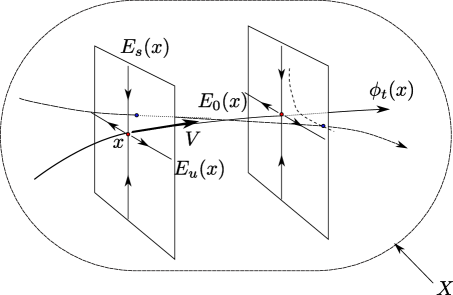
Figure 1: Picture of an Anosov flow in $X$ and instability of trajectories.

2.1 Remarks:

The remarks of this Section give more information on Anosov flows but are not necessary for the rest of this paper.

2.1.1 General remarks

• Standard examples of Anosov flows are suspensions of Anosov diffeomorphisms (see [36] p.8), or geodesic flows on manifolds $M$ with sectional negative curvature (see [36] p.9, or [28] p.549, p.551). Notice that in this case, the geodesic flow is Anosov on the unit cotangent bundle $X=T_{1}^{*}M$.

• The global hyperbolic structure of Anosov flows or Anosov diffeomorphisms is a very strong geometric property, so that manifolds carrying such dynamics satisfy strong topological conditions and the list of known examples is not so long. See [7] for a detailed discussion and references on that question.

• Let

  $$d_{u}=\dim E_{u}\left(x\right),\qquad d_{s}=\dim E_{s}\left(x\right),$$

  (they are independent of $x\in X$). Eq.(2) implies $d_{u}+d_{s}+1=\dim X=n$. For every $d_{u},d_{s}\geq 1$ one may construct an example of an Anosov flow: one considers a suspension of a hyperbolic diffeomorphism of $SL_{n-1}\left(\mathbb{Z}\right)$ on $\mathbb{T}^{n-1}$, with $n=d_{u}+d_{s}+1$, such that there are $d_{s}$ eigenvalues with modulus $\left|\lambda\right|<1$, and $d_{u}$ eigenvalues with modulus $\left|\lambda\right|>1$.

2.1.2 Constructive expressions for $E_{u}$, $E_{s}$

In the case where $d_{u}=d_{s}=1$, there is a formula which gives the distributions $E_{u},E_{s}$ [2]. Let $\left[v_{0}\right]\in C^{\infty}\left(\mathbb{P}\left(TX\right)\right)$ be a global smooth section of the projective tangent bundle, such that at every point $x\in X$, $\left[v_{0}\right]_{x}\notin\left(E_{0}\left(x\right)\oplus E_{s}\left(x\right)\right)$ (it is sufficient that the direction $\left[v_{0}\right]_{x}$ is close enough to the unstable direction $E_{u}\left(x\right)$). Then for every $x\in X$,

$$E_{u}\left(x\right)=\lim_{t\rightarrow+\infty}D\phi_{t}\left(\left[v_{0}\right]_{\phi_{-t}\left(x\right)}\right).$$ (4)

Similarly if $\left[v_{0}\right]_{x}\notin\left(E_{0}\left(x\right)\oplus E_{u}\left(x\right)\right),\forall x\in X$, then for every $x\in X$,

$$E_{s}\left(x\right)=\lim_{t\rightarrow-\infty}D\phi_{t}\left(\left[v_{0}\right]_{\phi_{-t}\left(x\right)}\right).$$

See figure 2.

Figure 2: Picture of the flow on the projective tangent bundle $\mathbb{P}\left(TX\right)$ induced by the hyperbolic vector field $V$. A global section $[v_{0}]$ will converge towards $E_{u}$ or $E_{s}$ for $t\rightarrow\pm\infty$ as explained in Eq.(4).

In the general case, for every $d_{u},d_{s}$, there exists a similar construction. Let $\left[v_{0}\right]\in C^{\infty}\left(\mbox{Gr}_{d_{u},n}\left(TX\right)\right)$ be a global smooth and non vanishing section of the Grassmanian bundle, such that at every point $x\in X$, the linear space $\left[v_{0}\right]_{x}$ does not intersect $E_{0}\left(x\right)\oplus E_{s}\left(x\right)$. Then for every $x\in X$,

$$E_{u}\left(x\right)=\lim_{t\rightarrow+\infty}D\phi_{t}\left(\left[v_{0}\right]_{\phi_{-t}\left(x\right)}\right).$$

Similarly

$$E_{s}\left(x\right)=\lim_{t\rightarrow-\infty}D\phi_{t}\left(\left[v_{0}\right]_{\phi_{-t}\left(x\right)}\right),$$

when $\left[v_{0}\right]\in C^{\infty}\left(\mbox{Gr}_{d_{s},n}\left(TX\right)\right)$ does not intersect $E_{0}\oplus E_{u}$.

2.1.3 Anosov one form $\alpha$ and regularity of the distributions $E_{u}\left(x\right)$, $E_{s}\left(x\right)$

The distribution $E_{0}\left(x\right)$ is smooth since $V\left(x\right)$ is assumed to be smooth. The distributions $E_{u}\left(x\right)$, $E_{s}\left(x\right)$ and $E_{u}\left(x\right)\oplus E_{s}\left(x\right)$ are only Hölder continuous in general (see [36] p.15, [21] p.211). Smoothness can be present with additional hypothesis or with particular models. See the discussion below, section 2.1.3 page 2.1.3.

The above hypothesis on the flow implies that there is a particular continuous one form on $X$, denoted $\alpha\in C^{0}\left(T^{*}X\right)$ called the Anosov 1-form and defined by

$$\mbox{ker}\left(\alpha\left(x\right)\right)=E_{u}\left(x\right)\oplus E_{s}\left(x\right),\qquad\left(\alpha\left(x\right)\right)\left(V\left(x\right)\right)=1,\qquad\forall x\in X.$$ (5)

Since $E_{u}$ and $E_{s}$ are invariant by the flow then $\alpha$ is invariant as well, $\phi_{t}^{*}\left(\alpha\right)=\alpha$ for every $t\in\mathbb{R}$, and therefore (in the sense of distributions)

$$\mathcal{L}_{V}\left(\alpha\right)=0,$$ (6)

where $\mathcal{L}_{V}$ denotes the Lie derivative.

We discuss now some known results about the smoothness of the distributions $E_{u}\left(x\right),E_{s}\left(x\right)$ in some special cases.

• In the case of a geodesic flow on a smooth Riemannian negative curvature manifold $M$ (with $X=T_{1}^{*}M$), $E_{u}\left(x\right)\oplus E_{s}\left(x\right)$ is orthogonal to $E_{0}\left(x\right)$, therefore $E_{u}\left(x\right)\oplus E_{s}\left(x\right)$ is $C^{\infty}$. The distributions $E_{u}\left(x\right)$, $E_{s}\left(x\right)$ are $C^{1}$ individually (see [20] p.252).

• More generally, the flow $\phi_{t}$ is a contact flow (or Reeb vector field, see [33] p.106, [41, p.55]) if the associated one form $\alpha$ defined in Eq.(5) is $C^{\infty}$ and if

  $$d\alpha_{/\left(E_{u}\oplus E_{s}\right)}\mbox{ is non degenerate (i.e. symplectic)}$$ (7)

  meaning that $\alpha$ is a contact one form. Equivalently, $dx:=\alpha\wedge\left(d\alpha\right)^{n}$ is a volume form on $X$ with $n:=\frac{1}{2}\dim\left(E_{u}\oplus E_{s}\right)$. Notice that (6) implies that the volume form is invariant by the flow:

  $$\mathcal{L}_{V}\left(dx\right)=0.$$ (8)

  In that case, $E_{u}\left(x\right)\oplus E_{s}\left(x\right)=\mbox{ker}\left(\alpha\right)$ is $C^{\infty}$ and $\alpha$ determines $V$ by $d\alpha\left(V\right)=0$ and $\alpha\left(V\right)=1$.

• (From [21] p.211) Hurder and Katok in [27] showed that if $\phi_{t}$ is an Anosov flow on $X$, $\mbox{dim}X=3$, and if $\alpha$ is a contact form of class $C^{1}$ then $\alpha$ is $C^{\infty}$ in fact, and $E_{u}\left(x\right)$, $E_{s}\left(x\right)$ are $C^{2-\varepsilon}$ for every $\varepsilon>0$. Moreover if $E_{u}\left(x\right),E_{s}\left(x\right)$ are $C^{2}$ then they are $C^{\infty}$ in fact and $C^{\infty}$ conjugated to an algebraic flow [20].

3 Transfer operator and the dynamics lifted on $T^{*}X$

3.1 The transfer operator

The flow $\phi_{t}$ acts in a natural manner on functions by pull back and this defines the transfer operator:

Definition 2.

The Ruelle transfer operator $\widehat{M}_{t}:C^{\infty}\left(X\right)\rightarrow C^{\infty}\left(X\right)$, $t\in\mathbb{R}$ is defined by: $$\widehat{M}_{t}\varphi=\varphi\circ\phi_{-t},\qquad\varphi\in C^{\infty}\left(X\right),$$ (9) $\widehat{M}_{t}$ can be expressed in terms of the vector field $V$ as $$\widehat{M}_{t}=\exp\left(-tV\right)=\exp\left(-it\widehat{H}\right)$$ (10) with the generator $$\widehat{H}:=-iV.$$ (11)

Remarks:

• If $dx$ is a smooth density on $X$, then $\widehat{M}_{t}$ can be extended to $L^{2}\left(X,dx\right)$. In this space, $\widehat{M}_{t}$ is a bounded operator. The adjoint of $\widehat{H}$ is ([47] prop.(2.4) p.129)

  $$\widehat{H}^{*}=-iV-i\,\mbox{div}\left(V\right)=\widehat{H}-i\,\mbox{div}\left(V\right).$$ (12)

  Hence ([47] def.(2.1) p.125)

  $$\mbox{div}\left(V\right)=0 \Leftrightarrow\mathcal{L}_{V}\left(dx\right)=0\Leftrightarrow \phi_{t}\mbox{ preserves }dx$$

  $$\Leftrightarrow \widehat{H}\mbox{ is self-adjoint on }L^{2}\left(X,dx\right)$$

  $$\Leftrightarrow \widehat{M}_{t}\mbox{ is a unitary operator on }L^{2}\left(X,dx\right).$$

  This is the case for the geodesic flow, which preserves the Liouville measure, or more generally for a contact flow from (8). But for a generic Anosov flow there does not exist any smooth invariant measure.

• From the probabilistic point of view, it is natural to consider the Perron Frobenius transfer operator $\widehat{T}_{t}$, $t\in\mathbb{R}$ whose generator is the adjoint $\widehat{H}^{*}$, Eq.(12):

  $$\widehat{T}_{t}:=e^{-i\widehat{H}^{*}t}=\left(\widehat{M}_{\left(-t\right)}\right)^{*}.$$ (14)

  The reason is that one has the following relation which is interpreted as a conservation of the total probability measure:

  $$\int_{X}\left(\widehat{T}_{t}\psi\right)dx=\int_{X}\psi dx,\qquad\psi\in C^{\infty}\left(X\right).$$

  Proof.

  $\int_{X}\left(\widehat{T}_{t}\psi\right)dx=\left(1|\widehat{T}_{t}\psi\right)=\left(\widehat{M}_{\left(-t\right)}1|\psi\right)=\int_{X}\psi dx$ since $\widehat{M}_{\left(-t\right)}1=1$ by (9). ∎

• We introduce the antilinear operator of complex conjugation $\widehat{C}:C^{\infty}\left(X\right)\rightarrow C^{\infty}\left(X\right)$ by

  $$\widehat{C}\varphi:=\overline{\varphi},\qquad\varphi\in C^{\infty}\left(X\right),$$ (15)

  which can be extended to $\mathcal{D}^{\prime}\left(X\right)$ by duality: for $\psi\in\mathcal{D}^{\prime}\left(X\right)$, $\varphi\in C^{\infty}\left(X\right)$,

  $$\langle\widehat{C}\psi|\varphi\rangle:=\overline{\langle\psi|\widehat{C}\varphi\rangle}.$$

  We have the following relation

  $$\widehat{H}\widehat{C}+\widehat{C}\widehat{H}=0$$ (16)

  (it will imply a symmetry for the Ruelle resonance spectrum, see Proposition 14 page 14)

  Proof.

  Since $V$ is real, for every $\varphi\in C^{\infty}\left(X\right)$ one has $\widehat{H}\widehat{C}\varphi=-iV\left(\overline{\varphi}\right)=\overline{iV\left(\varphi\right)}=-\overline{\left(-iV\left(\varphi\right)\right)}=-\widehat{C}\widehat{H}\varphi$. ∎

3.2 Generators of transfer operators are pseudo-differential operators

The generator $\widehat{H}$ defined in (11) is a differential operator hence a pseudodifferential operator. This allows us to use the machinery of semiclassical analysis in order to study the spectral properties [48, chap. 7]. In particular it allows us to view $\widehat{M}_{t}=\exp\left(-it\widehat{H}\right)$ as a Fourier integral operator. See proposition 4 below.

3.2.1 Symbols and pseudodifferential operators

In this Section we recall how pseudodifferential operators are defined from their symbols on a manifold $X$. We first recall [23, 48, p.2] that:

Definition 3.

The symbol class $S^{\mu}$ with order $\mu\in\mathbb{R}$ consist of $C^{\infty}$ functions $p\left(x,\xi\right)$ on $\mathbb{R}^{n}\times\mathbb{R}^{n}$ such that $$\forall\alpha,\beta,\quad\left|\partial_{\xi}^{\alpha}\partial_{x}^{\beta}p\right|\leq C_{\alpha,\beta}\left\langle\xi\right\rangle^{\mu-\left|\alpha\right|},\qquad\mbox{with }\left\langle\xi\right\rangle:=\sqrt{1+\xi^{2}}.$$ (17)

The value of $\mu$ governs the increase (or decrease) of $p\left(x,\xi\right)$ as $\left|\xi\right|\rightarrow\infty$.

On a manifold $X$ with a given system of coordinates (more precisely a chart system and a related partition of unity, see [48, p.30]), the symbol $p$ determines a pseudodifferential operator (PDO for short) denoted $\widehat{P}=\mathrm{Op}\left(p\right)$ acting on $u\in C^{\infty}\left(X\right)$ and defined locally by

$$\widehat{P}:u\rightarrow\left(\widehat{P}u\right)\left(x\right)=\int e^{i\xi\left(x-y\right)}p\left(x,\xi\right)u\left(y\right)dyd\xi.$$ (18)

Conversely $p=\sigma\left(\widehat{P}\right)$ is called the symbol of the PDO $\widehat{P}$. Notation: if $p\in S^{\mu}$ we say that $\widehat{P}\in\mathrm{Op}\left(S^{\mu}\right)$.

The value of the order $\mu$ is independent on the choice of coordinates, but the symbol $p$ of a given PDO $\widehat{P}$ depends on a choice of a chart and a choice of a partition of unity ([48, p.30]). The symbol has not a “geometrical meaning”. However it appears that the change of coordinate systems changes the symbol only at a subleading order $S^{\mu-1}$. In other words, the principal symbol $p_{ppal}=p\mbox{ mod }S^{\mu-1}$ is a well defined function on the manifold $X$ (independently of the charts).

Concerning the operator $\widehat{H}=-iV$ given in Eq.(11), one easily checks [47, p.2] that it is obtained by $\widehat{H}=\mathrm{Op}\left(H\right)$ with the symbol

$$H\left(x,\xi\right)=V\left(\xi\right)\in S^{1}.$$

Notice that this symbol does not depend on the chart. This is very particular to differential operators of order 1.

The quantization formula (18) is sometimes called the left-quantization or ordinary quantization of differential operators. There are plenty of other quantization formulae which differ at subleading order $\mathrm{Op}\left(S^{\mu-1}\right)$ so the principal symbol of a PDO is the same for the different quantizations. Some have interesting properties. For example the Weyl quantization of a symbol $p_{W}$ [48, (14.5) p.60] denoted by $\widehat{P}=\mathrm{Op}_{W}\left(p_{W}\right)$ is defined by:

$$\widehat{P}:u\rightarrow\left(\widehat{P}u\right)\left(x\right)=\int e^{i\xi\left(x-y\right)}p_{W}\left(\frac{x+y}{2},\xi\right)u\left(y\right)dyd\xi.$$ (19)

In this quantization, a real symbol $p_{W}$ is quantized as a formally self-adjoint operator.

In our example Eq.(11), $\widehat{H}=-iV$, the Weyl symbol is

$$H_{W}\left(x,\xi\right)=V\left(\xi\right)+\frac{i}{2}\mbox{div}\left(V\right).$$ (20)

Notice that this symbol does not depend on the choice of coordinates systems provided the volume form is expressed by $dx=dx_{1}\ldots\dot{dx_{n}}$. The term $\frac{i}{2}\mbox{div}\left(V\right)$ in (20) belongs to $S^{0}$ and is called the subprincipal symbol.

For general symbols and with the Weyl quantization, a change of coordinate systems preserving the volume form changes the symbol at a subleading order $S^{\mu-2}$ only. In other words, on a manifold with a fixed smooth density $dx$, the Weyl symbol $p_{W}$ of a given PDO $\widehat{P}$ is well defined modulo terms in $S^{\mu-2}$.

In this paper we will also use a Toeplitz quantization (or F.B.I. quantization) for the proof of Lemma 25 page 25.

3.2.2 Induced dynamics on $T^{*}X$

Recall that the canonical symplectic two form on $T^{*}X$ is ([33] p.90)

$$\omega:=d\xi\wedge dx.$$ (21)

The following well known proposition shows that the flow on the cotangent bundle $T^{*}X$ obtained by lifting the flow $\phi_{t}$ is naturally associated to the Ruelle transfer operator we are interesting in.

Proposition 4.

The symbol of the differential operator $\widehat{H}$ defined in Eq.(11) belongs to the symbol class $S^{1}$. Its principal symbol is equal to: $$H_{0}\left(x,\xi\right)=V\left(\xi\right)\in S^{1}.$$ (22) The Ruelle transfer operator $\widehat{M}_{t}$, defined in Eq.(10) is a semi-classical Fourier integral operator (FIO), whose associated canonical map denoted by $M_{t}:T^{*}X\rightarrow T^{*}X$ is the canonical lift of the diffeomorphism $\phi_{t}$ on $T^{*}X$ (linear in the fibers). See figure 3. More precisely if $x\in X$, $x^{\prime}=\phi_{t}\left(x\right)$ then $$M_{t}:\begin{cases}T^{*}X&\rightarrow T^{*}X\\ x&\longmapsto x^{\prime}=\phi_{t}\left(x\right)\\ \xi\in T_{x}^{*}X&\longmapsto\xi^{\prime}=\left(D_{x^{\prime}}\phi_{-t}\right)^{\mathrm{t}}\xi\in T_{x^{\prime}}^{*}X\end{cases}$$ (23) $M_{t}$ is also the Hamiltonian flow generated by the vector field $\mathbf{X}\in C^{\infty}\left(T^{*}X,T\left(T^{*}X\right)\right)$ defined by $$\omega\left(.,\mathbf{X}\right)=dH_{0}.$$ (24) The vector field $\mathbf{X}$ is the canonical lift of $V$ on $T^{*}X$.

Proof.

For (22), see [48] p.2. From (10), $\widehat{M}_{t}$ is defined by

$$i\frac{d\widehat{M}_{t}}{dt}=\widehat{H}\widehat{M}_{t},\qquad\widehat{M}_{t=0}=Id.$$

For (23) see [32, ex.2 p.152] or [47] Eq.(14.20) p. 77 and Eq.(14.15) p. 76, or [33], ex. 3.12 p.92. ∎

Figure 3: The flow $\phi_{t}$ generated by the vector field $V$ on $X$ is lifted on the cotangent bundle $T^{*}X$. This gives a Hamiltonian flow $M_{t}$ generated by a vector field $\mathbf{X}$.

Remarks:

• The Hamiltonian vector field $\mathbf{X}\in C^{\infty}\left(T^{*}X,T\left(T^{*}X\right)\right)$ can be expressed as usual with respect to a coordinate system by ([47, p.74])

  $$\mathbf{X}=\frac{\partial H_{0}}{\partial\xi}\frac{\partial}{\partial x}-\frac{\partial H_{0}}{\partial x}\frac{\partial}{\partial\xi}.$$

• From (12) the operators $\widehat{H}$ and $\widehat{H}^{*}$ have the same real principal symbol $H_{0}\left(x,\xi\right)=V\left(\xi\right)$. Therefore the canonical transform associated to the Perron Frobenius operator $\widehat{T}_{t}$ , Eq.(14), is also $M_{t}$.

3.2.3 Dual decomposition

Let

$$\boxed{T_{x}^{*}X=E_{u}^{*}\left(x\right)\oplus E_{s}^{*}\left(x\right)\oplus E_{0}^{*}\left(x\right)}$$ (25)

be the decomposition dual to (2) in the sense that

$$\left(E_{0}^{*}\left(x\right)\right)\left(E_{u}\left(x\right)\oplus E_{s}\left(x\right)\right) =0,$$ (26)

$$\left(E_{u}^{*}\left(x\right)\right)\left(E_{u}\left(x\right)\oplus E_{0}\left(x\right)\right)=0, \quad\left(E_{s}^{*}\left(x\right)\right)\left(E_{s}\left(x\right)\oplus E_{0}\left(x\right)\right)=0.$$

Remarks:

• Let us remark that we have exchanged $E_{u}^{*}$ and $E_{s}^{*}$ with respect to the usual definition of dual spaces. Our choice of notations will be justified by Eq.(29).

• One has

  $$\mbox{dim}E_{0}^{*}\left(x\right) =\mbox{dim}E_{0}\left(x\right)=1,$$

  $$\mbox{dim}E_{u}^{*}\left(x\right)=\mbox{dim}E_{s}\left(x\right)=d_{s}, \quad\mbox{dim}E_{s}^{*}\left(x\right)=\mbox{dim}E_{u}\left(x\right)=d_{u}.$$

• From (5) and (26), one deduces that $E_{0}^{*}$ is spanned by the one form $\alpha$:

  $$E_{0}^{*}\left(x\right)=\mathbb{R}\,\alpha\left(x\right).$$ (27)

• Notice that since $E_{u}\left(x\right)\oplus E_{s}\left(x\right)$ is not smooth in general (see remarks page 2.1), the same holds for $E_{0}^{*}\left(x\right)$. However $\left(E_{u}^{*}\left(x\right)\oplus E_{s}^{*}\left(x\right)\right)$ is smooth since $E_{0}\left(x\right)$ is smooth.

Definition 5.

For $E\in\mathbb{R}$, let $$\Sigma_{E}:=H_{0}^{-1}\left(E\right)\subset T^{*}X$$ (28) be the “energy shell” (where the function $H_{0}\left(x,\xi\right)=V\left(\xi\right)$ has been defined in (22)).

$\Sigma_{E}$ is a smooth hyper-surface in $T^{*}X$. More precisely for every $x\in X$,

$$\Sigma_{E}\left(x\right):=\Sigma_{E}\cap T_{x}^{*}X$$

is an affine hyperplane in $T_{x}^{*}X$, parallel to $E_{u}^{*}\left(x\right)\oplus E_{s}^{*}\left(x\right)$ and therefore transverse to $E_{0}^{*}\left(x\right)$. See Figure 4.

Figure 4: Picture of $T_{x}^{*}X$ for a given $x\in X$, and a given $E\in\mathbb{R}$.

Proposition 6.

The decomposition (25) is invariant by the flow $M_{t}$ and there exists $c>0,\theta>0$ such that $\displaystyle\left|M_{t}\left(\xi_{s}\right)\right|$ $\displaystyle\leq$ $\displaystyle ce^{-\theta t}\left|\xi_{s}\right|,\qquad\forall\xi_{s}\in E_{s}^{*},\quad\forall t\geq 0,$ (29) $\displaystyle\left|M_{t}\left(\xi_{u}\right)\right|$ $\displaystyle\leq$ $\displaystyle ce^{-\theta\left|t\right|}\left|\xi_{u}\right|,\qquad\forall\xi_{u}\in E_{u}^{*},\quad\forall t\leq 0.$ For every $E\in\mathbb{R}$, the energy shell $\Sigma_{E}$ is invariant by the flow $M_{t}$. In the energy shell $\Sigma_{E}$ the trapped set $K_{E}$ is defined by $$K_{E}:=\left\{K_{E}\left(x\right)=\left(\Sigma_{E}\left(x\right)\cap E_{0}^{*}\left(x\right)\right),\qquad x\in X\right\}.$$ (30) $K_{E}$ is a global continuous section of the cotangent bundle $T^{*}X$ given in terms of the associated one form (5) by: $$K_{E}=E\alpha.$$ In general $K_{E}\left(x\right)$ is not smooth but only Hölder continuous (as $E_{0}^{*}\left(x\right)$). $K_{E}$ is globally invariant under the flow $M_{t}$.

Proof.

By duality with what happens in $TX$ described in (3). Since $\alpha\left(V\right)=1$ then $H_{0}\left(\alpha\right)=V\left(\alpha\right)=1$. Therefore $\alpha\in\Sigma_{E=1}$. Also $\alpha\in E_{0}^{*}$ therefore $\alpha=K_{E=1}$. ∎

Remarks:

• In general the trapped set $K$ is defined by:

  $$K:=\left\{\left(x,\xi\right)\in T^{*}X,\quad\exists C>0;\forall t\in\mathbb{R},\left|M_{t}\left(x,\xi\right)\right|\leq C\right\},$$

  i.e. $K$ contains trajectories which do not escape towards infinity neither in the future nor in the past. We have:

  $$K=\bigcup_{E\in\mathbb{R}}K_{E}=E_{0}^{*}.$$

• Notice that for every $E\in\mathbb{R}$ the trapped set $K_{E}$ is a sub-manifold of $T^{*}X$ homeomorphic to $X$ hence compact. This observation is at the origin of the method to prove the existence of discrete resonance spectrum below (Theorem 12). The dynamics of $M_{t}$ restricted to $K_{E}$ is conjugated to the dynamics of $\phi_{t}$ on $X$ (it is a lift of $\phi_{t}$ on $K_{E}$).

• For the special case of a contact flow on $X$ with a $C^{\infty}$ contact 1 form $\alpha$ then $K_{E=1}=\alpha$ and therefore $K_{E}=E\alpha$ is a $C^{\infty}$ section. The restriction of the canonical two form (21) to this section (seen as a submanifold of $T^{*}X$) is

  $$\omega_{/K_{E}}=E\left(\pi^{*}\left(d\alpha\right)\right)_{/K_{E}},$$ (31)

  where $\pi:T^{*}X\rightarrow X$ is the bundle projection. We observe that $K\backslash\left\{\xi=0\right\}$ is a smooth symplectic submanifold of $T^{*}X$ (far from being a Lagrangian submanifold of $T^{*}X$), $\left(K_{E},E\xi dx\right)$ is a contact manifold for $E\neq 0$ isomorphic to $\left(X,E\alpha\right)$.

3.3 The escape function

In this section we construct a smooth function $G_{m}$ on the cotangent space $T^{*}X$ called the escape function. We will denote $\frac{\xi}{\left|\xi\right|}$ the direction of a cotangent vector $\xi$ and $S^{*}X:=\left(T^{*}X\backslash\left\{0\right\}\right)/\mathbb{R}^{+}$ the cosphere bundle which is the bundle of directions of cotangent vectors $\xi/\left|\xi\right|$. $S^{*}X$ is a compact space. The images of $E_{u}^{*},E_{s}^{*},E_{0}^{*}\subset T^{*}X$ by the projection $T^{*}X\backslash\left\{0\right\}\rightarrow S^{*}X$ are denoted respectively $\widetilde{E}_{u}^{*},\widetilde{E}_{s}^{*},\widetilde{E}_{0}^{*}\subset S^{*}X$, see Figure 5(a) page 5.

Lemma 7.

Let $u,n_{0},s\in\mathbb{R}$ with $u<n_{0}<s$. There exists a smooth function $m\left(x,\xi\right)\in C^{\infty}\left(T^{*}X\right)$ called an “order function”, taking values in the interval $\left[u,s\right]$, and an “escape function” on $T^{*}X$ defined by: $$G_{m}\left(x,\xi\right):=m\left(x,\xi\right)\log\sqrt{1+\left(f\left(x,\xi\right)\right)^{2}},$$ (32) where $f\in C^{\infty}\left(T^{*}X\right)$ and for $\left|\xi\right|\geq 1$, $f>0$ is positively homogeneous of degree 1 in $\xi$. $f\left(x,\xi\right)=\left|\xi\right|$ in a conical neighborhood of $E_{u}^{*}$ and $E_{s}^{*}$. $f\left(x,\xi\right)=H_{0}\left(x,\xi\right)$ in a conical neighborhood of $E_{0}^{*}$, such that: 1. For $\left|\xi\right|\geq 1$, $m\left(x,\xi\right)$ depends only on the direction $\frac{\xi}{\left|\xi\right|}\in S_{x}^{*}X$ and takes the value $u$ (respect. $n_{0},s$) in a small neighborhood of $E_{u}^{*}$ (respect. $E_{0}^{*},E_{s}^{*}$). See figure 5(a). 2. $G_{m}$ decreases strictly and uniformly along the trajectories of the flow $M_{t}$ in the cotangent space, except in a conical vicinity $\widetilde{N}_{0}$ of the neutral direction $E_{0}^{*}$ and for small $\left|\xi\right|$: there exists $R>0$ such that $$\forall x\in X,\,\forall\left|\xi\right|\geq R,\,\frac{\xi}{\left|\xi\right|}\notin\widetilde{N}_{0}\qquad\mathbf{X}\left(G_{m}\right)\left(x,\xi\right)<-C_{m}<0,$$ (33) with $$C_{m}:=c\min\left(\left|u\right|,s\right)$$ (34) and $c>0$ independent of $u,n_{0},s$. 3. More generally $$\forall x\in X,\,\forall\left|\xi\right|\geq R,\qquad\mathbf{X}\left(G_{m}\right)\left(x,\xi\right)\leq 0.$$ (35) See figure 5(b).

            

Figure 5: (a) The induced flow $\widetilde{M}_{t}$ on the cosphere bundle $S^{*}X:=\left(T^{*}X\backslash\left\{0\right\}\right)/\mathbb{R}^{+}$ which is the bundle of directions of cotangent vectors $\xi/\left|\xi\right|$. (Here the picture is restricted to a fiber $S_{x}^{*}X$).
(b) Picture in the cotangent space $T_{x}^{*}X$ which shows in grey the sets outside of which the escape estimate (33) holds.

Remarks

• It is important to notice that we can choose $m$ such that the value of $C_{m}$ is arbitrarily large (by making $s,\left|u\right|\rightarrow\infty$) and that the neighborhood $\widetilde{N}_{0}$ is arbitrarily small.

• The value of $n_{0}$ could be chosen to be $n_{0}=0$ to simplify. But it is interesting to observe that letting $n_{0},s\rightarrow+\infty$, the order function $m\left(x,\xi\right)$ can be made arbitrarily large for $\left|\xi\right|\geq 1$, outside a small vicinity of $E_{u}^{*}$. We will use this in the proof of Theorem 13 in order to show that the wavefront of the eigen-distributions are included in $E_{u}^{*}$.

• Inspection of the proof shows that with an adapted norm $\left|\xi\right|$ obtained by averaging, $c$ can be chosen arbitrarily close to $\theta$, defined in (29).

• The constancy of $m$ in the vicinity of the stable/unstable/neutral directions allows us to have a smooth escape function $G_{m}$ although the distributions $E_{s}^{*}\left(x\right)$,$E_{u}^{*}\left(x\right)$,$E_{0}^{*}\left(x\right)$ have only Hölder regularity in general.

3.3.1 Proof of Lemma 7

We first define a function $m\left(x,\xi\right)$ called the order function following closely [17] Section 3.1 (and [19] p.196).

The function $m$.

The following Lemma is useful for the construction of escape functions. Let $M$ be a compact manifold and let $v$ be a smooth vector field on $M$. We denote $\mathrm{exp}\left(tv\right):M\rightarrow M$ the flow at time $t$ generated by $v$. Let $\Sigma_{u}$, $\Sigma_{s}$ be compact disjoint subsets of $M$ such that

$$\mathrm{dist\,}(\exp\left(tv\right)(\rho),\Sigma_{s})\to 0,\ t\to+\infty\mbox{ when }\rho\in M\setminus\Sigma_{u}$$

$$\mathrm{dist\,}(\exp\left(tv\right)(\rho),\Sigma_{u})\to 0,\ t\to-\infty\mbox{ when }\rho\in M\setminus\Sigma_{s}.$$

Lemma 8.

Let $V_{u},V_{s}\subset M$ be open neighborhoods of $\Sigma_{u}$ and $\Sigma_{s}$ respectively and let $\varepsilon>0$. Then there exist $W_{u}\subset V_{u}$, $W_{s}\subset V_{s}$, $m\in C^{\infty}(M;[0,1])$, $\eta>0$ such that $v(m)\geq 0$ on $M$, $v(m)>\eta>0$ on $M\setminus\left(W_{u}\cup W_{s}\right)$, $m\left(\rho\right)>1-\varepsilon$ for $\rho\in W_{s}$ and $m\left(\rho\right)<\varepsilon$ for $\rho\in W_{u}$.

Proof.

After shrinking $V_{u},V_{s}$ we may assume that $V_{u}\cap V_{s}=\emptyset$ and

$$t\geq 0\Rightarrow\exp\left(tv\right)(V_{s})\subset V_{s},\mbox{ and }t\leq 0\Rightarrow\exp\left(tv\right)(V_{u})\subset V_{u}.$$ (36)

Let $T>0$ and let $W_{s}:=M\backslash\mathrm{exp}\left(Tv\right)\left(V_{u}\right)=\mathrm{exp}\left(Tv\right)\left(M\backslash V_{u}\right)$ and $W_{u}:=M\backslash\mathrm{exp}\left(-Tv\right)\left(V_{s}\right)=\mathrm{exp}\left(-Tv\right)\left(M\backslash V_{s}\right)$. See figure 6.

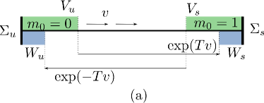
Figure 6: Illustration for the proof of Lemma 8. The horizontal axis is a schematic picture of $M$ and this shows the construction and properties of the sets $V_{u},V_{s}$ and $W_{u},W_{s}$.

If $T$ is large enough one has $W_{u}\subset V_{u}$, $W_{s}\subset V_{s}$ and $W_{s}\cap W_{u}=\emptyset$. Let $m_{0}\in C^{\infty}(M;[0,1])$ be equal to 1 on $V_{s}$ and equal to 0 on $V_{u}$. Put

$$m=\frac{1}{2T}\int_{-T}^{T}m_{0}\circ\exp\left(tv\right)\,dt.$$ (37)

Then

$$v(m)(\rho)=\frac{1}{2T}\left(m_{0}\left(\exp\left(Tv\right)\left(\rho\right)\right)-m_{0}\left(\exp\left(-Tv\right)\left(\rho\right)\right)\right).$$ (38)

• Let $\rho\in M\setminus\left(W_{u}\cup W_{s}\right)$. From (38) we see that $v\left(m\right)\left(\rho\right)=\frac{1}{2T}(1-0))=\frac{1}{2T}>0$.

For $\rho\in M$ let

$$\mathcal{I}\left(\rho\right):=\left\{t\in\mathbb{R},\mathrm{exp}\left(tv\right)\left(\rho\right)\in M\backslash\left(V_{u}\cup V_{s}\right)\right\}.$$

This is a closed connected interval by (36) and moreover its length is uniformly bounded:

$$\exists\tau>0,\quad\forall\rho\in M,\quad\left|\mathrm{max}\left(\mathcal{I}\left(\rho\right)\right)-\mathrm{min}\left(\mathcal{I}\left(\rho\right)\right)\right|\leq\tau.$$

In other words, $\tau$ is an upper bound for the travel time in the domain $M\backslash\left(V_{u}\cup V_{s}\right)$.

To prove the Lemma, we have to consider two more cases:

• Let $\rho\in W_{u}$. If $t\leq T-\tau$ then $m_{0}\left(\mbox{exp}\left(tv\right)\left(\rho\right)\right)=0$ and

  $$m\left(\rho\right)=\frac{1}{2T}\left(\int_{-T}^{T-\tau}\underbrace{m_{0}\left(\exp\left(tv\right)\rho\right)}_{=0}dt+\int_{T-\tau}^{T}\underbrace{m_{0}\left(\exp\left(tv\right)\rho\right)}_{\leq 1}dt\right)\leq\frac{\tau}{2T}<\varepsilon,$$

  where the last inequality holds if one chooses $T$ large enough. One has $m_{0}\left(\exp\left(-Tv\right)\left(\rho\right)\right)=0$ therefore (38) implies that $v(m)(\rho)\geq 0$.

• Let $\rho\in W_{s}$. One shows similarly that

  $$m\left(\rho\right)=\frac{1}{2T}\left(\int_{-T}^{-T+\tau}\underbrace{m_{0}\left(\exp\left(tv\right)\rho\right)}_{\geq 0}dt+\int_{-T+\tau}^{T}\underbrace{m_{0}\left(\exp\left(tv\right)\rho\right)}_{=1}dt\right)\geq\frac{2T-\tau}{2T}>1-\varepsilon,$$

  for $T$ large enough, and $v(m)(\rho)\geq 0$.

∎

We now apply Lemma 8 to the case when $M=S^{*}X$ and $v$ is the image $\widetilde{\mathbf{X}}$ on $S^{*}X$ of our Hamilton field $\mathbf{X}$. See figure 7.

• We first take $\Sigma_{u}=\Sigma_{u}^{1}=\widetilde{E}_{s}^{*}$ and let $\Sigma_{s}=\Sigma_{s}^{1}\subset M$ be the set of limit points $\lim_{j\to+\infty}\exp t_{j}v(\rho)$, where $\rho\in M\setminus\Sigma_{u}^{1}$ and $t_{j}\to+\infty$. $\Sigma_{s}^{1}$ is the union of $\widetilde{E}_{0}^{*}$, $\widetilde{E}_{u}^{*}$ and all trajectories $\exp(\mathbb{R}v)(\rho)$ where $\rho$ has the property that $\exp tv(\rho)$ converges to $\widetilde{E}_{0}^{*}$ when $t\to-\infty$ and to $\widetilde{E}_{u}^{*}$ when $t\to+\infty$. Equivalently, $\Sigma_{s}^{1}$ is the image $\widetilde{E_{u}^{*}\oplus E_{0}^{*}}$ in $S^{*}X$ of $E_{u}^{*}\oplus E_{0}^{*}$. Applying the Lemma, we get $m_{1}=m\in C^{\infty}(M;[0,1])$ such that $m_{1}<\varepsilon$ outside an arbitrarily small neighborhood $W_{u}^{1}$ of $\Sigma_{u}^{1}=\widetilde{E}_{s}^{*}$, $m_{1}>1-\varepsilon$ outside an arbitrarily small neighborhood $W_{s}^{1}$ of $\Sigma_{s}^{1}=\widetilde{E_{u}^{*}\oplus E_{0}^{*}}$ and $\widetilde{\mathbf{X}}(m_{1})\geq 0$ everywhere with strict inequality $\widetilde{\mathbf{X}}(m_{1})>\eta>0$ outside $W_{s}^{1}\cup W_{u}^{1}$.

• Similarly, we can find $m_{2}=m\in C^{\infty}(M;[0,1])$, such that $m_{2}<\varepsilon$ outside an arbitrarily small neighborhood $W_{u}^{2}$ of $\Sigma_{u}^{2}=\widetilde{E_{s}\oplus E_{0}^{*}}$, $m_{2}>1-\varepsilon$ outside an arbitrarily small neighborhood $W_{s}^{2}$ of $\Sigma_{s}^{2}=\widetilde{E}_{u}^{*}$ and $\widetilde{\mathbf{X}}(m_{2})\geq 0$ everywhere with strict inequality $\widetilde{\mathbf{X}}(m_{2})>\eta>0$ outside $W_{s}^{2}\cup W_{u}^{2}$.

Figure 7: Representation of different sets on $S^{*}X$ used in the proof.

Let $u<n_{0}<s$ and put

$$\widetilde{m}:=s+\left(n_{0}-s\right)m_{1}+\left(u-n_{0}\right)m_{2},$$

$$\widetilde{N}_{s}:=W_{u}^{1}\cap W_{u}^{2},\quad\widetilde{N}_{0}:=W_{s}^{1}\cap W_{u}^{2},\quad\widetilde{N}_{u}:=W_{s}^{1}\cap W_{s}^{2}.$$

Then

• on $S^{*}X\backslash\left(\widetilde{N}_{s}\cup\widetilde{N}_{0}\cup\widetilde{N}_{u}\right)=\left(S^{*}X\backslash\left(W_{u}^{1}\cup W_{s}^{1}\right)\right)\cup\left(S^{*}X\backslash\left(W_{u}^{2}\cup W_{s}^{2}\right)\right)$ we have $\widetilde{\mathbf{X}}\left(m_{1}\right)>\eta$ or $\widetilde{\mathbf{X}}\left(m_{2}\right)>\eta$ therefore

  $$\widetilde{\mathbf{X}}\left(\widetilde{m}\right) =\left(n_{0}-s\right)\widetilde{\mathbf{X}}\left(m_{1}\right)+\left(u-n_{0}\right)\widetilde{\mathbf{X}}\left(m_{2}\right)$$ (39)

  $$<-\eta\min\left(\left|n_{0}-s\right|,\left|u-n_{0}\right|\right).$$

• on $\widetilde{N}_{s}=W_{u}^{1}\cap W_{u}^{2}$ we have $m_{1}<\varepsilon$ and $m_{2}<\varepsilon$ therefore

  $$\widetilde{m} >s+\left(n_{0}-s\right)\varepsilon+\left(u-n_{0}\right)\varepsilon$$

  $$=s\left(1-\varepsilon\right)+u\varepsilon>\frac{s}{2},$$ (40)

  where the last inequality holds if $\varepsilon$ is chosen small enough.

• on $\widetilde{N}_{u}=W_{s}^{1}\cap W_{s}^{2}$ we have $m_{1}>1-\varepsilon$ and $m_{2}>1-\varepsilon$ therefore

  $$\widetilde{m} <s+\left(n_{0}-s\right)\left(1-\varepsilon\right)+\left(u-n_{0}\right)\left(1-\varepsilon\right)$$

  $$=\varepsilon s+u\left(1-\varepsilon\right)<\frac{u}{2},$$ (41)

  where the last inequality holds if $\varepsilon$ is chosen small enough.

• on $S^{*}X$ we have

  $$\widetilde{\mathbf{X}}\left(\widetilde{m}\right)=\left(n_{0}-s\right)\widetilde{\mathbf{X}}\left(m_{1}\right)+\left(u-n_{0}\right)\widetilde{\mathbf{X}}\left(m_{2}\right)\leq 0.$$ (42)

We construct a smooth function $m$ on $T^{*}M$ satisfying

$$m\left(x,\xi\right) = \widetilde{m}\left(\frac{\xi}{\left|\xi\right|}\right),\qquad\mbox{if }\left|\xi\right|\geq 1,$$

$$= 0\qquad\mbox{if }\left|\xi\right|\leq 1/2.$$

The symbol $G_{m}$.

Let

$$G_{m}\left(x,\xi\right):=m\left(x,\xi\right)\log\sqrt{1+\left(f\left(x,\xi\right)\right)^{2}}$$

with $f\in C^{\infty}\left(T^{*}X\right)$ such that for $\left|\xi\right|\geq 1$, $f>0$ is positively homogeneous of degree 1 in $\xi$, and

$$\frac{\xi}{\left|\xi\right|}\in\widetilde{N}_{u}\cup\widetilde{N}_{s}\Rightarrow f\left(x,\xi\right):=\left|\xi\right|$$

$$\frac{\xi}{\left|\xi\right|}\in\widetilde{N}_{0}\Rightarrow f\left(x,\xi\right):=H_{0}\left(x,\xi\right).$$

The consequences of these choices are:

• Since $\mathbf{X}\left(H_{0}\right)=0$ then $\mathbf{X}\left(\log\sqrt{1+\left(f\left(x,\xi\right)\right)^{2}}\right)=0$ for $\frac{\xi}{\left|\xi\right|}\in\widetilde{N}_{0}$.

• Since $E_{s}^{*}$ is the stable direction and $E_{u}^{*}$ the unstable one,

  $$\exists C>0,\qquad\frac{\xi}{\left|\xi\right|}\in\widetilde{N}_{s}\Rightarrow\mathbf{X}\left(\log\left\langle\xi\right\rangle\right)<-C,\qquad\frac{\xi}{\left|\xi\right|}\in\widetilde{N}_{u}\Rightarrow\mathbf{X}\left(\log\left\langle\xi\right\rangle\right)>C.$$ (43)

  Notice that by averaging, the norm $\left|\xi\right|$ can be chosen such that for $\left|\xi\right|$ large enough, $C$ is arbitrarily closed to $\theta$ defined in (29).

• In general $\left|\mathbf{X}\left(\log\sqrt{1+f^{2}}\right)\right|$ is bounded:

  $$\exists C_{2}>0,\qquad\forall\xi\in T^{*}X,\quad\left|\mathbf{X}\left(\log\sqrt{1+\left(f\left(x,\xi\right)\right)^{2}}\right)\right|<C_{2}.$$

We will show now the uniform escape estimate Eq.(33) page (33). One has

$$\mathbf{X}\left(G_{m}\right)=\mathbf{X}\left(m\right)\log\sqrt{1+f^{2}}+m\mathbf{X}\left(\log\sqrt{1+f^{2}}\right).$$ (44)

We will first consider each term separately assuming $\left|\xi\right|\geq 1$.

• If $\widetilde{\xi}\in S^{*}X\setminus\left(\widetilde{N}_{s}\cup\widetilde{N}_{u}\cup\widetilde{N}_{0}\right)$ then using (39) and the fact that $\left|\mathbf{X}\left(\log\sqrt{1+f^{2}}\right)\right|$ and $m$ are bounded, one has for $\left|\xi\right|$ large enough

  $$\mathbf{X}\left(G_{m}\right)\left(x,\xi\right)<-c\min\left(s,\left|u\right|\right)$$

  with $c>0$ independent of $u,n_{0},s$.

• If $\widetilde{\xi}\in\widetilde{N}_{u}$ then from (43) and (41) there exists $c>0$ such that

  $$\mathbf{X}\left(G_{m}\right)=\underbrace{\mathbf{X}\left(m\right)}_{\leq 0}\underbrace{\log\left\langle\xi\right\rangle}_{\geq 0}+\underbrace{m}_{<\frac{u}{2}}\underbrace{\mathbf{X}\left(\log\left\langle\xi\right\rangle\right)}_{>C}<-c\left|u\right|<0.$$

• If $\widetilde{\xi}\in\widetilde{N}_{s}$ then from (43) and (40) there exists $c>0$ such that

  $$\mathbf{X}\left(G_{m}\right)=\underbrace{\mathbf{X}\left(m\right)}_{\leq 0}\underbrace{\log\left\langle\xi\right\rangle}_{\geq 0}+\underbrace{m}_{>\frac{s}{2}}\underbrace{\mathbf{X}\left(\log\left\langle\xi\right\rangle\right)}_{<-C}<-cs<0.$$

We have obtained the uniform escape estimate Eq.(33) page 33. Finally for $\widetilde{\xi}\in\widetilde{N}_{0}$, we have

$$\mathbf{X}\left(G_{m}\right)=\underbrace{\mathbf{X}\left(m\right)}_{\leq 0}\underbrace{\log\sqrt{1+f^{2}}}_{\geq 0}+m\underbrace{\mathbf{X}\left(\log\sqrt{1+f^{2}}\right)}_{=0}\leq 0,$$

and we deduce (35) page 35. We have finished the proof of Lemma 7 page 7.

4 Spectrum of resonances

In this Section we give our main results about the spectrum of the generator $\widehat{H}$, Eq(11), in specific Sobolev spaces. We first define these Sobolev spaces.

4.1 Anisotropic Sobolev spaces

4.1.1 Symbol classes with variable order

The escape function $G_{m}$ defined in Lemma 7 has some regularity expressed by the fact that it belongs to some symbol classes $S^{\mu}$. This will allow us to perform some semiclassical calculus. In this section, we describe these symbol classes.

Lemma 9.

The order function $m\left(x,\xi\right)$ defined in in Lemma 7 belongs to $S^{0}$ ( definition 3 page 3). The escape function $G_{m}$ defined in (32) belongs to the symbol class $S^{\mu}$ for every $\mu>0$. For short, we will write $G_{m}\in S^{+0}$.

In the paper [17, Appendix] we have shown that the order function $m\left(x,\xi\right)\in S^{0}$ can be used to define the class $S_{\rho}^{m\left(x,\xi\right)}$ of symbols of variable order $m\left(x,\xi\right)$. We recall the definition:

Definition 10.

Let $m\left(x,\xi\right)\in S^{0}$ and $\frac{1}{2}<\rho\leq 1$. A function $p\in C^{\infty}\left(T^{*}X\right)$ belongs to the class $S_{\rho}^{m\left(x,\xi\right)}$ of variable order if for every trivialization $\left(x,\xi\right):\left.T^{*}X\right|_{U}\rightarrow\mathbb{R}^{2n}$, for every compact $K\subset U$ and all multi-indices $\alpha,\beta\in\mathbb{N}^{n}$, there is a constant $C_{K,\alpha,\beta}$ such that $$\left|\partial_{\xi}^{\alpha}\partial_{x}^{\beta}p\left(x,\xi\right)\right|\leq C_{K,\alpha,\beta}\left\langle\xi\right\rangle^{m\left(x,\xi\right)-\rho\left|\alpha\right|+\left(1-\rho\right)\left|\beta\right|}$$ (45) for every $\left(x,\xi\right)\in\left.T^{*}X\right|_{U}$.

We refer to [17, Section A.2.2] for a precise description of semiclassical theorems related to symbols with variable orders.

Proposition 11.

The operator $$\widehat{A}_{m}:=\mathrm{Op}\left(\exp\left(G_{m}\right)\right)$$ (46) is a PDO whose symbol belongs to the class $S_{\rho}^{m\left(x,\xi\right)}$ for every $\rho<1$ (we write $S_{1-0}^{m\left(x,\xi\right)}$ for short). Its principal symbol is $$A_{m}\left(x,\xi\right)=e^{G_{m}\left(x,\xi\right)}=\left\langle\xi\right\rangle^{m\left(x,\xi\right)}.$$ The symbol $A_{m}$ can be modified at a subleading order (i.e. $S_{\rho}^{m\left(x,\xi\right)-\left(2\rho-1\right)}$) such that the operator becomes formally self-adjoint and invertible on $C^{\infty}\left(X\right)$.

Remark: one can also show that $A_{m}\in S_{1}^{m\left(x,\xi\right)+0}$ but this is less precise than $A_{m}\in S_{1-0}^{m\left(x,\xi\right)}$.

Proof.

We refer to the appendix in the paper [17, Lemma 6]. ∎

4.1.2 Anisotropic Sobolev spaces

For every order function $m$ as in Lemma 7, we define the anisotropic Sobolev space $H^{m}$ to be the space of distributions (included in $\mathcal{D}^{\prime}\left(X\right)$):

$$\boxed{H^{m}:=\widehat{A}_{m}^{-1}\left(L^{2}\left(X\right)\right).}$$ (47)

Some basic properties of the space $H^{m}$, such as embedding properties, are given in [17, section 3.2].

The generator $\widehat{H}=-iV$ , Eq.(11), is defined by duality on the distribution space $\mathcal{D}^{\prime}\left(X\right)$ and we can therefore consider its restriction to the anisotropic Sobolev space $H^{m}$.

4.2 Main results on the spectrum of Ruelle resonances

The following theorem 12 has been obtained in [10, Theorem 1] (with the slight difference that the authors use Banach spaces) . In particular we refer to this paper for results and discussions concerning the SRB measure. We provide a new proof below, based on semiclassical analysis in the spirit of the paper [17].

Theorem 12.

“Discrete spectrum”. Let $m$ be a function which satisfies the hypothesis of Lemma 7 page 7. The generator $\widehat{H}=-iV$ , Eq.(11), defines by duality an unbounded operator on the anisotropic Sobolev space $H^{m}$ , Eq.(47), $$\widehat{H}:H^{m}\rightarrow H^{m}$$ in the sense of distributions with domain given by $$\mathcal{D}\left(\widehat{H}\right):=\left\{\varphi\in H^{m},\quad\widehat{H}\varphi\in H^{m}\right\}.$$ It coincides with the closure of $\left(-iV\right):C^{\infty}\rightarrow C^{\infty}$ in the graph norm for operators. For $z\in\mathbb{C}$ such that $\Im\left(z\right)>-\left(C_{m}-C\right)$ with $C_{m}$ defined in (34) and some $C$ independent of $m$, the operator $\left(\widehat{H}-z\right):\mathcal{D}\left(\widehat{H}\right)\cap H^{m}\rightarrow H^{m}$ is a Fredholm operator with index $0$ depending analytically on $z$. Recall that $C_{m}$ is arbitrarily large. Consequently the operator $\widehat{H}$ has a discrete spectrum in the domain $\Im\left(z\right)>-\left(C_{m}-C\right)$, consisting of eigenvalues $\lambda_{i}$ of finite algebraic multiplicity. See Figure 8. Moreover, $\widehat{H}$ has no spectrum in the half plane $\Im\left(z\right)>0$.

Concerning Fredholm operators we refer to [12, p.122] or [25, Appendix A p.220]. The proof of Theorem 12 is given page 4.3.

The next Theorem show that the spectrum is intrinsic and describes the wavefront of the eigenfunctions associated to $\lambda_{i}$. The wavefront of a distribution has been introduced by Hörmander. See for instance [23, p.77] of [48, p.27] for the definition. The wavefront corresponds to the directions in $T^{*}X$ where the distribution is not $C^{\infty}$.

Theorem 13.

”The discrete spectrum is intrinsic to the Anosov vector field”. More precisely, let $\widetilde{m},\widetilde{f}$, $\widetilde{G}_{m}=\widetilde{m}\log\sqrt{1+\widetilde{f}^{2}}$ be another set of functions as in Lemma 7 so that Theorem 12 applies and $\widehat{H}:H^{\widetilde{m}}\rightarrow H^{\widetilde{m}}$ has discrete spectrum in the set $\Im\left(z\right)>-\left(\widetilde{C}_{\widetilde{m}}-\widetilde{C}\right)$. Then in the set $\Im\left(z\right)>-\min\left(\left(C_{m}-C\right),\left(\widetilde{C}_{\widetilde{m}}-\widetilde{C}\right)\right)$ the eigenvalues of $\widehat{H}:H^{m}\rightarrow H^{m}$ counted with their multiplicity and their respective eigenspaces coincide with those of $\widehat{H}:H^{\widetilde{m}}\rightarrow H^{\widetilde{m}}$. The eigenvalues $\lambda_{i}$ are called the Ruelle Resonances and we denote the set by $\mathrm{Res}\left(\widehat{H}\right)$. The wavefront of the associated generalized eigenfunctions is contained in the unstable direction $E_{u}^{*}$. The resolvent $\left(z-\widehat{H}\right)^{-1}$ viewed as an operator $C^{\infty}\left(X\right)\rightarrow\mathcal{D}^{\prime}\left(X\right)$ has a meromorphic extension from $\Im\left(z\right)\gg 1$ to $\mathbb{C}$. The poles of this extension are the Ruelle resonances.

The proof of Theorem 13 is given page 4.4.

The following proposition is a very simple observation.

Proposition 14.

”Symmetry”. The order function $m$ can be chosen such that $m\left(x,-\xi\right)=m\left(x,\xi\right)$. Then the conjugation operator $\widehat{C}$ defined in (15) leaves the space $H^{m}$ invariant. If $\widehat{H}\psi=\lambda\psi$, $\psi\in H^{m}$ then $\widetilde{\psi}:=\widehat{C}\psi\in H^{m}$ is also an eigenfunction with eigenvalue $\widetilde{\lambda}=-\overline{\lambda}$. The spectrum of Ruelle resonances is therefore symmetric with respect to the imaginary axis.

Proof.

of Proposition 14. We first have to show that the space $H^{m}\left(X\right)=\widehat{A}^{-1}\left(L^{2}\left(X\right)\right)$ is invariant by $\widehat{C}$, equivalently that $L^{2}\left(X\right)$ is invariant by $\widehat{A}\widehat{C}\widehat{A}^{-1}$. Notice that $\widehat{C}$ is an “anti-linear FIO” whose associated transformation is $C:\left(x,\xi\right)\rightarrow\left(x,-\xi\right)$, which is anti-canonical since $C^{*}\omega=-\omega$. The symbol $A\left(x,\xi\right)$ is invariant under the map $C:\left(x,\xi\right)\rightarrow\left(x,-\xi\right)$. One can therefore construct $\widehat{A}$ such that $\widehat{C}\widehat{A}\widehat{C}=\widehat{A}$. Since $\widehat{C}\widehat{A}\widehat{C}=\widehat{A}$$\Leftrightarrow\widehat{A}\widehat{C}\widehat{A}^{-1}=\widehat{C}$ and since the space $L^{2}\left(X\right)$ is invariant under $\widehat{C}$, we conclude that $L^{2}\left(X\right)$ is invariant by $\widehat{A}\widehat{C}\widehat{A}^{-1}$. Finally if $\widehat{H}\psi=\lambda\psi$, $\psi\in H^{m}$, let $\widetilde{\psi}=\widehat{C}\psi\in H^{m}$. Then using (16), $\widehat{H}\widetilde{\psi}=\widehat{H}\widehat{C}\psi=-\widehat{C}\widehat{H}\psi=-\overline{\lambda}\widetilde{\psi}$. ∎

Here is the new result of this paper:

Theorem 15.

“Semiclassical upper bound for the density of resonances”. For every $E\in\mathbb{R}\backslash\left\{0\right\},$ every $\beta>0$, in the semiclassical limit $\alpha\rightarrow+\infty$ we have $$\sharp\left\{\lambda\in\mathrm{Res}\left(\widehat{H}\right),\,\,\left|\Re\left(\lambda\right)-E\alpha\right|\leq\sqrt{\alpha},\,\,\Im\left(\lambda\right)>-\beta\right\}\leq o\left(\alpha^{n-1/2}\right),$$ (48) with $n=\dim X$.

Figure 8: Spectrum of Ruelle resonances of $\widehat{H}=-iV$. From Theorem 15 the number of eigenvalues in the rectangle is $o\left(\alpha^{n-1/2}\right)$ for $\alpha\rightarrow\infty$.

Remarks:

• Notice that by a simple scaling in $\alpha$ we can reduce the values of $E$ to $E=\pm 1$ in Theorem 15.

• The case $E=0$ is excluded in Theorem 15 because the vicinity of the origin $\xi=0$ is excluded in (35). If one were able to construct an escape function such that in addition $\mathbf{X}\left(G_{m}\right)\left(x,\xi\right)\leq C$, $\forall\left(x,\xi\right)$, with some $C$ independent of $m$ then $E=0$ would not be excluded.

• We recall a simple and well known result (which follows from the property that $\left\|\widehat{M}_{t}\right\|_{\infty}=1$), that there is no eigenvalue in the upper half plane and no Jordan block on the real axis .

• The upper bound given in (48) results from our method and choice of escape function $A\left(x,\xi\right)$. In the proof, $o\left(\alpha^{n-1/2}\right)$ comes from a symplectic volume $\mathcal{V}$ in phase space which contains the trapped set $\Sigma_{E}$ and which is of order $\mathcal{V}\simeq\delta\alpha^{-1/2}$, with $\delta$ arbitrarily small. Using Weyl inequalities we obtain an upper bound of order $\alpha^{n}\mathcal{V}\simeq\delta\alpha^{n-1/2}$ in (48). It is expected that a better choice of the escape function could improve this upper bound. For specific models, e.g. geodesic flows on a surface with constant negative curvature, it is known that the upper bound is $O\left(\alpha^{\frac{n}{2}}\right)$ (see [29]). We reasonably expect this in general.

• From the upper bound (48), one can deduce upper bounds in larger spectral domains. For example: for every $\beta>0$, in the semiclassical limit $\alpha\rightarrow+\infty$ we have

  $$\sharp\left\{\lambda\in\mathrm{Res}\left(\widehat{H}\right),\,\,\Re\left(\lambda\right)\in\left[-\alpha,\alpha\right],\,\,\Im\left(\lambda\right)>-\beta\right\}\leq o\left(\alpha^{n}\right),$$

  with $n=\dim X$.

4.3 Proof of theorem 12 about the discrete spectrum of resonances

Here are the different steps that we will follow in the proof.

1. The operator $\widehat{H}$ on the Sobolev space $H^{m}=\widehat{A}_{m}^{-1}\left(L^{2}\left(X\right)\right)$ is unitarily isomorphic to the operator $\widehat{P}:=\widehat{A}_{m}\widehat{H}\widehat{A}_{m}^{-1}$ on $L^{2}\left(X\right)$. We will show that $\widehat{P}$ is a pseudo-differential operator. We will compute the symbol $P\left(x,\xi\right)$ of $\widehat{P}$ in Lemma 16. The important fact is that the derivative of the escape function appears in the imaginary part of the symbol $P\left(x,\xi\right)$.

2. For $\Im\left(z\right)\gg 1$, using the Gårding inequality, we will show that $\left(\widehat{P}-z\right)$ is invertible and therefore that $\widehat{P}$ has no spectrum in the domain $\Im\left(z\right)\gg 1$.

3. Using the Gårding inequality again for a modified operator and analytic Fredholm theory we will show that $\left(\widehat{P}-z\right)$ is invertible for $\Im\left(z\right)>-\left(C_{m}-C\right)$ for some constant $C$ independent of $m$, except for a discrete set of points $z=\lambda_{i}$ with finite multiplicity.

4.3.1 Conjugation by the escape function and unique closed extension of $\widehat{P}$ on $L^{2}\left(X\right)$

Let us define

$$\boxed{\widehat{P}:=\widehat{A}_{m}\widehat{H}\widehat{A}_{m}^{-1}.}$$ (49)

The following commuting diagram shows that the operator $\widehat{P}$ on $L^{2}\left(X\right)$ is unitarily equivalent to $\widehat{H}$ on $H^{m}$.

$$\begin{array}[]{ccc}L^{2}\left(X\right)&\overset{\widehat{P}}{\rightarrow}&L^{2}\left(X\right)\\ \downarrow\widehat{A}_{m}^{-1}&\circlearrowleft&\downarrow\widehat{A}_{m}^{-1}\\ H^{m}&\overset{\widehat{H}}{\rightarrow}&H^{m}\end{array}$$

The definitions of symbol classes $S^{\mu}$ and $S_{\rho}^{m}$ are given in Sections 3.2.1 and 4.1.1. In the following Lemma, the notation $\mathcal{O}_{m}\left(S^{-1+0}\right)$ means that the term is a symbol in $S^{-1+0}$. We add the index $m$ to emphasize that it depends on the escape function $m$ whereas $\mathcal{O}\left(S^{0}\right)$ means that the term is a symbol in $S^{0}$ which does not depend on $m$.

Lemma 16.

The operator $\widehat{P}$ defined in (49) is a PDO in $\mathrm{Op}\left(S^{1}\right)$. With respect to every given system of coordinates its symbol is equal to $$P\left(x,\xi\right)=H\left(x,\xi\right)+i\left(\mathbf{X}\left(G_{m}\right)\right)\left(x,\xi\right)+\mathcal{O}_{m}\left(S^{-1+0}\right),$$ (50) where $H\left(x,\xi\right)$ is the symbol of $\widehat{H}$: $$H\left(x,\xi\right)=V\left(\xi\right)+\mathcal{O}\left(S^{0}\right),$$ with principal symbol $V\left(\xi\right)\in S^{1}$, see Eq.(22), and $\mathbf{X}\left(G_{m}\right)\in S^{+0}$. $\mathbf{X}$ is the Hamiltonian vector field of $H$ defined in (24).

Proof.

The proof consists in making the following two lines precise and rigorous:

$$\widehat{P} =\widehat{A}\widehat{H}\widehat{A}^{-1}=\mathrm{Op}\left(e^{G_{m}}\right)\widehat{H}\left(\mathrm{Op}\left(e^{G_{m}}\right)\right)^{-1}\simeq\left(1+\mathrm{Op}\left(G_{m}\right)+\ldots\right)\widehat{H}\left(1-\mathrm{Op}\left(G_{m}\right)+\ldots\right)$$

$$=\widehat{H}+\left[\mathrm{Op}\left(G_{m}\right),\widehat{H}\right]+\ldots=\mathrm{Op}\left(H-i\left\{G_{m},H\right\}+\ldots\right)=\mathrm{Op}\left(H+i\mathbf{X}\left(G_{m}\right)+\ldots\right).$$

In order to avoid to work with exponentials of operators, let us define

$$\widehat{A}_{m,t}:=\mathrm{Op}\left(e^{tG_{m}}\right)=\mathrm{Op}\left(e^{G_{tm}}\right)=\widehat{A}_{tm},\qquad 0\leq t\leq 1,$$

and

$$\widehat{H}_{m,t}:=\widehat{A}_{m,t}\widehat{H}\widehat{A}_{m,t}^{-1}$$

which interpolates between $\widehat{H}=\widehat{H}_{m,0}$ and $\widehat{P}=\widehat{H}_{m,1}$. We have seen in Lemma 9 that $\widehat{G}_{m}\in\mathrm{Op}\left(S^{+0}\right)$, in Proposition 11 that $\widehat{A}_{m,t}\in\mathrm{Op}\left(S^{tm\left(x,\xi\right)+0}\right)$, $\widehat{A}_{m,t}^{-1}\in\mathrm{Op}\left(S^{-tm\left(x,\xi\right)+0}\right)$ and in Eq.(22) that $\widehat{H}\in\mathrm{Op}\left(S^{1}\right)$. We deduce that $\widehat{H}_{m,t}\in\mathrm{Op}\left(S^{1+0}\right)$. Then

$$\frac{d\widehat{A}_{m,t}}{dt}=\mathrm{Op}\left(G_{m}e^{tG_{m}}\right)=\mathrm{Op}\left(G_{m}\right)\mathrm{Op}\left(e^{tG_{m}}\right)+\mathcal{O}_{m}\left(\mathrm{Op}\left(S^{tm-1+0}\right)\right)$$

$$\left(\frac{d\widehat{A}_{m,t}}{dt}\right)\widehat{A}_{m,t}^{-1}=-\widehat{A}_{m,t}\left(\frac{d\widehat{A}_{m,t}^{-1}}{dt}\right)=\mathrm{Op}\left(G_{m}+r_{m,t}\right)$$

with $r_{m,t}\in S^{-1+0}$ and

$$\frac{d}{dt}\widehat{H}_{m,t} =\left(\frac{d\widehat{A}_{m,t}}{dt}\widehat{A}_{m,t}^{-1}\right)\widehat{A}_{m,t}\widehat{H}\widehat{A}_{m,t}^{-1}+\widehat{A}_{m,t}\widehat{H}\widehat{A}_{m,t}^{-1}\left(\widehat{A}_{m,t}\frac{d\widehat{A}_{m,t}^{-1}}{dt}\right)$$

$$=\left[\mathrm{Op}\left(G_{m}+r_{m,t}\right),\widehat{H}_{m,t}\right]\in\mathrm{Op}\left(S^{+0}\right).$$

Therefore $\widehat{H}_{m,t}-\widehat{H}=\left(\int_{0}^{t}\frac{d}{ds}\widehat{H}_{m,s}ds\right)\in\mathrm{Op}\left(S^{+0}\right)$ and

$$\frac{d}{dt}\widehat{H}_{m,t} =\left[\mathrm{Op}\left(G_{m}\right),\widehat{H}\right]+\left[\mathrm{Op}\left(r_{m,t}\right),\widehat{H}\right]+\left[\mathrm{Op}\left(G_{m}+r_{m,t}\right),\widehat{H}_{m,t}-\widehat{H}\right]$$

$$=\left[\mathrm{Op}\left(G_{m}\right),\widehat{H}\right]+\mathcal{O}_{m}\left(\mathrm{Op}\left(S^{-1+0}\right)\right).$$

We deduce that

$$\widehat{P}=\widehat{H}+\left(\int_{0}^{1}\frac{d}{dt}\widehat{H}_{m,t}dt\right)=\widehat{H}+\left[\mathrm{Op}\left(G_{m}\right),\widehat{H}\right]+\mathcal{O}_{m}\left(\mathrm{Op}\left(S^{-1+0}\right)\right).$$

Since

$$\left[\mathrm{Op}\left(G_{m}\right),\widehat{H}\right]=\mathrm{Op}\left(i\left(\mathbf{X}\left(G_{m}\right)\right)\left(x,\xi\right)+\mathcal{O}_{m}\left(S^{-1+0}\right)\right),$$

we get

$$\widehat{P}=\widehat{H}+\mathrm{Op}\left(i\left(\mathbf{X}\left(G_{m}\right)\right)\left(x,\xi\right)+\mathcal{O}_{m}\left(S^{-1+0}\right)\right).$$

Finally since $\widehat{H}=\mathrm{Op}\left(V\left(\xi\right)+\mathcal{O}\left(S^{0}\right)\right)$ with a remainder in $S^{0}$ which depends on the quantization (see discussion in Section 3.2.1) but which is independent of the escape function $m$, we get (50). Notice that with Weyl quantization, Eq. (20), the term $\mathcal{O}\left(S^{0}\right)$ is precisely equal to $\frac{i}{2}\mbox{div}\left(V\right)$. ∎

We have shown that $\widehat{P}$ is a unbounded PDO of order 1 that we may first equip with the domain $C^{\infty}\left(X\right)$ which is dense in $L^{2}\left(X\right)$. Lemma 29 page 29 shows that $\widehat{P}$ has a unique closed extension as an unbounded operator $\widehat{P}$ on $L^{2}\left(X\right)$. The adjoint $\widehat{P}^{*}$ is also a PDO of order 1 and it is the unique closed extension from $C^{\infty}\left(X\right)$.

4.3.2 $\widehat{P}$ has empty spectrum for $\Im\left(z\right)\gg 1$.

Let us write

$$\widehat{P}=\widehat{P}_{1}+i\widehat{P}_{2}$$

with $\widehat{P}_{1}:=\frac{1}{2}\left(\widehat{P}+\widehat{P}^{*}\right)$, $\widehat{P}_{2}:=\frac{i}{2}\left(\widehat{P}^{*}-\widehat{P}\right)$ self-adjoint. From (50) and (35), the symbol of the operator $\widehat{P}_{2}$ is

$$P_{2}\left(x,\xi\right)=\mathbf{X}\left(G_{m}\right)\left(x,\xi\right)+\mathcal{O}\left(S^{0}\right)+\mathcal{O}_{m}\left(S^{-1+0}\right)$$ (51)

belongs to $S^{+0}$ and satisfies

$$\exists C_{0},\forall\left(x,\xi\right),\quad\Re\left(P_{2}\left(x,\xi\right)\right)\leq C_{0}.$$

From the sharp Gårding inequality (95) page 95 applied here with order $\mu=1$ (since $P_{2}\in S^{+0}\subset S^{1}$) we deduce that there exists $C>0$ such that $\left(\widehat{P}_{2}u|u\right)\leq\left(C_{0}+C\right)\left\|u\right\|^{2}$ which writes:

$$\left(\widehat{P}_{2}-\left(C_{0}+C\right)u|u\right)\leq 0.$$ (52)

Lemma 17.

From the inequality (52) we deduce that for every $z\in\mathbb{C}$, $\Im\left(z\right)>C+C_{0}$, the resolvent $\left(\widehat{P}-z\right)^{-1}$ exists. Therefore $\widehat{P}$ has empty spectrum for $\Im\left(z\right)>C+C_{0}$.

Proof.

Let $\varepsilon=\Im\left(z\right)-\left(C_{0}+C\right)>0$. Then for $u\in C^{\infty}\left(X\right)$,

$$\Im\left(\left(\widehat{P}-z\right)u|u\right)=\left(\left(\widehat{P}_{2}-\left(C_{0}+C\right)\right)u|u\right)-\left(\Im\left(z\right)-\left(C_{0}+C\right)\right)\left\|u\right\|^{2}\leq-\varepsilon\left\|u\right\|^{2}.$$

Using Cauchy-Schwarz inequality,

$$\left\|\left(\widehat{P}-z\right)u\right\|\left\|u\right\|\geq\left|\left(\left(\widehat{P}-z\right)u|u\right)\right|\geq\left|\Im\left(\left(\widehat{P}-z\right)u|u\right)\right|\geq\varepsilon\left\|u\right\|^{2}.$$

Hence for $u\in C^{\infty}\left(X\right)$

$$\left\|\left(\widehat{P}-z\right)u\right\|\geq\varepsilon\left\|u\right\|.$$ (53)

By density this extends to all $u\in\mathcal{D}\left(\widehat{P}\right)$ and it follows that $\widehat{P}-z$ is injective with closed range $\mathcal{R}\left(\widehat{P}-z\right)$.

The same argument for the adjoint $\widehat{P}^{*}=\widehat{P}_{1}-i\widehat{P}_{2}$ gives

$$\left\|\left(\widehat{P}^{*}-\overline{z}\right)u\right\|\geq\varepsilon\left\|u\right\|,\qquad\forall u\in\mathcal{D}\left(\widehat{P}^{*}\right),$$ (54)

so $\widehat{P}^{*}-\overline{z}$ is also injective. If $u\in L^{2}\left(X\right)$ is orthogonal to $\mathcal{R}\left(\widehat{P}-z\right)$ then $u$ belongs to the kernel of $\widehat{P}^{*}-\overline{z}$ which is $0$. Hence $\mathcal{R}\left(\widehat{P}-z\right)=L^{2}\left(X\right)$ and $\widehat{P}-z:\mathcal{D}\left(\widehat{P}\right)\rightarrow L^{2}\left(X\right)$ is bijective with bounded inverses. ∎

4.3.3 The spectrum of $\widehat{P}$ is discrete on $\Im\left(z\right)\geq-\left(C_{m}-C\right)$ with some $C\geq 0$ independent of $m$.

As usual [38, p.113], in order to obtain a discrete spectrum for the operator $\widehat{P}$, we need to construct a relatively compact perturbation $\widehat{\chi}$ of the operator such that $\left(\widehat{P}-i\widehat{\chi}\right)$ has no spectrum on $\Im\left(z\right)\geq-\left(C_{m}-C\right)$.

Let $\chi_{0}:T^{*}X\rightarrow\mathbb{R}^{+}$ be a smooth non negative function with $\chi_{0}\left(x,\xi\right)=C_{m}>0$ for $\left(x,\xi\right)\in\widetilde{N}_{0}$ and $\chi_{0}\left(x,\xi\right)=0$ outside a neighborhood of $\widetilde{N}_{0}$ where $R$ and $\widetilde{N}_{0}$ are defined in Eq.(33) page 33. See also figure 5 (b). We can assume that $\chi_{0}\in S^{0}$.

Let $\widehat{\chi}_{0}:=\mathrm{Op}\left(\chi_{0}\right)$. We can assume that $\widehat{\chi}_{0}$ is self-adjoint. From Eq.(33), for every $\left(x,\xi\right)\in T^{*}X$, $\left|\xi\right|\geq R$,

$$\left(\mathbf{X}\left(G_{m}\right)\left(x,\xi\right)-\chi_{0}\left(x,\xi\right)\right)\leq-C_{m},$$

hence (51) gives for every $\left(x,\xi\right)\in T^{*}X$:

$$P_{2}\left(x,\xi\right)-\chi_{0}\left(x,\xi\right)\leq-C_{m}+C+\mathcal{O}_{m}\left(S^{-1+0}\right),$$

with some $C\in\mathbb{R}$ independent of $m$, coming from the $\mathcal{O}\left(S^{0}\right)$ term in (51). Notice that the remainder term $\mathcal{O}_{m}\left(S^{-1+0}\right)$ could be bounded but by a constant which depends on $m$.

Since $P_{2}\in S^{\mu}$ with every order $0<\mu<1$, the sharp Gårding inequality (95) page 95 implies that for every $u\in C^{\infty}\left(X\right)$ there exists $C_{\mu}>0$ such that

$$\left(\left(\widehat{P}_{2}-\widehat{\chi}_{0}+\left(C_{m}-C\right)\right)u|u\right)\leq C_{\mu}\left\|u\right\|_{H^{\frac{\mu-1}{2}}}^{2}.$$

The right hand side can be written $C_{\mu}\left\|u\right\|_{H^{\frac{\mu-1}{2}}}^{2}=C_{\mu}\left(\left\langle\widehat{\xi}\right\rangle^{\mu-1}u|u\right)=\Im\left(i\widehat{\chi}_{1}u|u\right)$ with $\widehat{\chi}_{1}=\mathrm{Op}\left(\chi_{1}\right)$, $\chi_{1}=C_{\mu}\left\langle\xi\right\rangle^{\mu-1}\in S^{\mu-1}$ and can be absorbed on the left by defining

$$\chi:=\chi_{0}+\chi_{1},\qquad\widehat{\chi}:=\mathrm{Op}\left(\chi\right).$$

We can assume that $\widehat{\chi}$ is self-adjoint. We obtain:

$$\left(\left(\widehat{P}_{2}-\widehat{\chi}+\left(C_{m}-C\right)\right)u|u\right)\leq 0.$$

As in the proof of Lemma 17 page 17 we obtain that the resolvent $\left(\widehat{P}-i\widehat{\chi}-z\right)^{-1}$ exists for $\Im\left(z\right)>-\left(C_{m}-C\right)$. The following lemma is the central observation for the proof of Theorem 12.

Lemma 18.

For every $z\in\mathbb{C}$ such that $\Im\left(z\right)>-\left(C_{m}-C\right)$, the operator $\widehat{\chi}\left(\widehat{P}-i\widehat{\chi}-z\right)^{-1}$ is compact.

Proof.

On the cone $\widetilde{N}_{0}$, the operator $\left(\widehat{P}-i\widehat{\chi}-z\right)$ is elliptic of order 1. We can therefore invert it micro-locally on $\widetilde{N}_{0}$, namely construct $E\in S^{-1}$ and $R_{1},R_{2}\in S^{0}$ such that

$$\left(\widehat{P}-i\widehat{\chi}-z\right)\widehat{E}=1+\widehat{R}_{1},\qquad\widehat{E}\left(\widehat{P}-i\widehat{\chi}-z\right)=1+\widehat{R}_{2},$$ (55)

$$\forall j=1,2,\qquad\mathrm{WF}\left(\widehat{R}_{j}\right)\cap\widetilde{N}_{0}=\emptyset.$$

In particular $\mathrm{WF}\left(\chi\widehat{R}_{j}\right)=\emptyset$ therefore $\widehat{\chi}\widehat{R}_{2}$ is a compact operator. Also $\widehat{E}$ is a compact operator (since $E\in S^{-1}$). Then from (55), we write:

$$\left(\widehat{P}-i\chi-z\right)^{-1}=\widehat{E}-\widehat{R}_{2}\left(\widehat{P}-i\widehat{\chi}-z\right)^{-1},$$

$$\widehat{\chi}\left(\widehat{P}-i\widehat{\chi}-z\right)^{-1}=\underbrace{\widehat{\chi}}_{bounded}\underbrace{\widehat{E}}_{compact}-\underbrace{\widehat{\chi}\widehat{R}_{2}}_{compact}\underbrace{\left(\widehat{P}-i\chi-z\right)^{-1}}_{bounded},$$

and deduce that $\widehat{\chi}\left(\widehat{P}-i\widehat{\chi}-z\right)^{-1}$ is a compact operator. ∎

With the following Lemma we finish the proof of Theorem 12.

Lemma 19.

From the facts that for every $z\in\mathbb{C},\Im\left(z\right)>-\left(C_{m}-C\right)$, $\left(\widehat{P}-i\widehat{\chi}-z\right)$ is invertible, $\widehat{\chi}\left(\widehat{P}-i\widehat{\chi}-z\right)^{-1}$ is compact and that $\left(\widehat{P}-z_{0}\right)$ is invertible for at least one point $z_{0}\in D$, we deduce that $\widehat{P}$ has discrete spectrum with locally finite multiplicity on $\Im\left(z\right)>-\left(C_{m}-C\right)$.

Proof.

Write for $\Im\left(z\right)>-\left(C_{m}-C\right)$:

$$\widehat{P}-z=\left(1+i\widehat{\chi}\left(\widehat{P}-i\widehat{\chi}-z\right)^{-1}\right)\left(\widehat{P}-i\widehat{\chi}-z\right).$$

Here $\left(\widehat{P}-i\widehat{\chi}-z\right):\mathcal{D}\left(\widehat{P}\right)\rightarrow L^{2}\left(X\right)$ is bijective with bounded inverse and hence Fredholm of index $0$. Similarly $\left(1+i\widehat{\chi}\left(\widehat{P}-i\widehat{\chi}-z\right)^{-1}\right):L^{2}\left(X\right)\rightarrow L^{2}\left(X\right)$ is Fredholm of index $0$ by Lemma 18. Thus

$$\widehat{P}-z:\mathcal{D}\left(\widehat{P}\right)\rightarrow L^{2}\left(X\right),\qquad\Im\left(z\right)>C_{m}-C,$$

is a holomorphic family of Fredholm operators (of index $0$) invertible for $\Im\left(z\right)\gg 0$. It then suffices to apply the analytic Fredholm theorem ([37, p.201, case (b)], see also [25, p.220 Appendix A]). ∎

4.4 Proof of theorem 13 that the eigenvalues are intrinsic to the Anosov vector field $V$

Let $m$ and $G_{m}$ be as in Lemma 7. Let $\widehat{m}=f\left(m\right)$ where $f\in C^{\infty}\left(\mathbb{R}\right)$, $f\left(t\right)\geq\max\left(0,t\right)$, $f^{\prime}\geq 0$, $f\left(t\right)=0$ for $t\leq u/2$ and $f\left(t\right)=t$ for $t\geq s/2$. $\widehat{H}$ viewed as a closed unbounded operator in $H^{\widehat{m}}$ has no spectrum in the half plane $\Im\left(z\right)\geq C_{1}$ for $C_{1}\gg 0$. The same holds for $\widehat{H}:L^{2}\rightarrow L^{2}$. Since $\widehat{m}\geq 0$ we have $H^{\widehat{m}}\subset L^{2}$ so if $v\in H^{\widehat{m}}$ then $R_{L^{2}}\left(z\right)v=R_{H^{\widehat{m}}}\left(z\right)v$ for $\Im\left(z\right)\geq C_{1}$ where $R_{L^{2}}$ denotes the resolvent of $\widehat{H}:L^{2}\rightarrow L^{2}$ and similarly for $R_{H^{\widehat{m}}}$.

Since $\widehat{m}\geq m$ we also have $H^{\widehat{m}}\subset H^{m}$ and hence $R_{H^{\widehat{m}}}\left(z\right)v=R_{H^{m}}\left(z\right)v$ for $\Im\left(z\right)\geq C_{1}$, $v\in H^{\widehat{m}}$. Especially when $v\in C^{\infty}$, we get $R_{L^{2}}\left(z\right)v=R_{H^{m}}\left(z\right)v$, $\Im\left(z\right)\geq C_{1}$. Applying Theorem 12, we conclude that $R_{L^{2}}\left(z\right)$, viewed as an operator $C^{\infty}\rightarrow\mathcal{D}^{\prime}$ has a meromorphic extension $R\left(z\right)$ from the half plane $\Im\left(z\right)\geq C_{1}$ to the half plane $\Im\left(z\right)>-\left(C_{m}-C\right)$ which coincide with $R_{H^{m}}$ restricted to $C^{\infty}$.

If $\gamma$ is a simple positively oriented closed curve in the half plane $\Im\left(z\right)>-\left(C_{m}-C\right)$ which avoids the eigenvalues of $\widehat{H}:H^{m}\rightarrow H^{m}$ then the spectral projection, associated to the spectrum of $\widehat{H}$ inside $\gamma$, is given by

$$\pi_{\gamma}^{H^{m}}=\frac{1}{2\pi i}\int_{\gamma}R_{H^{m}}\left(z\right)dz.$$

For $v\in C^{\infty}$, we have

$$\pi_{\gamma}^{H^{m}}v=\pi_{\gamma}v:=\frac{1}{2\pi i}\left(\int_{\gamma}R_{H^{m}}\left(z\right)dz\right)v.$$

Now $C^{\infty}$ is dense in $H^{m}$ and $\pi_{\gamma}^{H^{m}}$ is of finite rank, hence its range $\pi_{\gamma}^{H^{m}}\left(H^{m}\right)$ is equal to the image $\pi_{\gamma}\left(C^{\infty}\right)$ of $C^{\infty}$. The latter space is independent of the choice of $H^{m}$. More precisely if $\widetilde{m},\widetilde{f}$ are as in Theorem 12 and we choose $\gamma$ as above, now in the half plane $\Im\left(z\right)>-\min\left(\left(C_{m}-C\right),\left(C_{\widetilde{m}}-C\right)\right)$ and avoiding the spectrum of $\widehat{H}:H^{m}\rightarrow H^{m}$ and $\widehat{H}:H^{\widetilde{m}}\rightarrow H^{\widetilde{m}}$, then the spectral projections $\pi_{\gamma}^{H^{m}}$ and $\pi_{\gamma}^{H^{\widetilde{m}}}$ have the same range.

Since one can find order functions $m$ which are arbitrarily large in every direction except $E_{u}^{*}$, see remark 3.3 page 3.3, we deduce that the eigen-distributions are smooth in every direction except $E_{u}^{*}$. The Theorem follows.

4.5 Proof of theorem 15 for the upper bound on the density of resonances

The asymptotic regime $\Re\left(z\right)\gg 1$ which is considered in Theorem 15 is a semiclassical regime in the sense that it involves large values of $H\left(\xi\right)=V\left(\xi\right)\gg 1$, hence large values of $\left|\xi\right|$ in the cotangent space $T^{*}X$.

For convenience, we will switch to $h$-semiclassical analysis. Let $0<h\ll 1$ be a small parameter (we will set $\alpha=1/h$ in Theorem 15). In $h$-semiclassical analysis the symbol $\xi$ will be quantized into the operator $\mathrm{Op}_{h}\left(\xi\right):=hD_{x}=-ih\partial/\partial x$ whereas for ordinary PDO, $\xi$ is quantized into $\mathrm{Op}\left(\xi\right):=D_{x}=-i\partial/\partial x$. This is simply a rescaling of the cotangent space $T^{*}X$ by a factor $h$, i.e.

$$h\,\mathrm{Op}\left(\xi\right)=\mathrm{Op}_{h}\left(\xi\right).$$ (56)

In this Section we first recall the definition of symbols in $h$-semiclassical analysis. In Lemma 22 we derive again the expression of the symbol of $\widehat{P}$. In Section 4.5.3 we give the main idea of the proof and the next Sections give the details of this proof.

4.5.1 $h$-semiclassical class of symbols

We first define the symbol classes we will need in $h$-semiclassical analysis.

Definition 20.

The symbol class $\left(h^{-k}S_{\rho}^{\mu}\right)$ with $1/2<\rho\leq 1$, order $\mu\in\mathbb{R}$ and $k\in\mathbb{R}$ consists of $C^{\infty}$ functions $p\left(x,\xi;h\right)$ on $T^{*}X$, indexed by $0<h\ll 1$ such that in every trivialization $\left(x,\xi\right):\left.T^{*}X\right|_{U}\rightarrow\mathbb{R}^{2n}$, for every compact $K\subset U$ $$\forall\alpha,\beta,\quad\left|\partial_{\xi}^{\alpha}\partial_{x}^{\beta}p\right|\leq C_{K,\alpha,\beta}h^{-k+\left(\rho-1\right)\left(\left|\alpha\right|+\left|\beta\right|\right)}\left\langle\xi\right\rangle^{\mu-\rho\left|\alpha\right|+\left(1-\rho\right)\left|\beta\right|}.$$ (57)

For short we will write $S_{\rho}^{\mu}$ instead of $\left(h^{-k}S_{\rho}^{\mu}\right)$ when $k=0$, and write $S^{\mu}$ instead of $S_{\rho}^{\mu}$ when $\rho=1$.

For symbols of variable orders we have:

Definition 21.

Let $m\left(x,\xi\right)\in S^{0}$, $\frac{1}{2}<\rho\leq 1$ and $k\in\mathbb{R}$. A family of functions $p\left(x,\xi;h\right)\in C^{\infty}\left(T^{*}X\right)$ indexed by $0<h\ll 1$, belongs to the class $\left(h^{-k}S_{\rho}^{m\left(x,\xi\right)}\right)$ of variable order if in every trivialization $\left(x,\xi\right):\left.T^{*}X\right|_{U}\rightarrow\mathbb{R}^{2n}$, for every compact $K\subset U$ and all multi-indices $\alpha,\beta\in\mathbb{N}^{n}$, there is a constant $C_{K,\alpha,\beta}$ such that $$\left|\partial_{\xi}^{\alpha}\partial_{x}^{\beta}p\left(x,\xi\right)\right|\leq C_{K,\alpha,\beta}h^{-k-\left(1-\rho\right)\left(\left|\alpha\right|+\left|\beta\right|\right)}\left\langle\xi\right\rangle^{m\left(x,\xi\right)-\rho\left|\alpha\right|+\left(1-\rho\right)\left|\beta\right|},$$ (58) for every $\left(x,\xi\right)\in\left.T^{*}X\right|_{U}$.

4.5.2 The symbol of the conjugated operator

Since the symbol $H=V\left(\xi\right)\mbox{ mod }S^{0}$ of $\widehat{H}$, given in (22), is linear in $\xi$, it follows from (56) that

$$h\widehat{H}=h\mathrm{Op}\left(H\right)=\mathrm{Op}_{h}\left(H\right).$$

Therefore we also rescale the spectral domain $z\in\mathbb{C}$ by defining:

$$z_{h}:=hz,\qquad\widehat{H}_{h}:=h\widehat{H}.$$ (59)

and get

$$\widehat{H}_{h}=\mathrm{Op}_{h}\left(V\left(\xi\right)+\mathcal{O}\left(hS^{0}\right)\right)\quad\in\mathrm{Op}_{h}\left(S^{1}\right).$$

From now on we will work with these new variables and we will often drop the indices $h$ for short.

We will take again the escape function to be $G_{m}\left(x,\xi\right):=m\left(x,\xi\right)\log\left\langle\xi\right\rangle$ as in (32) but with the rescaled variable $\xi$, i.e. quantized by

$$\widehat{G}_{m}:=\mathrm{Op}_{h}\left(G_{m}\right).$$

Since the vector field $\mathbf{X}$ is linear in the fibers of the bundle $T^{*}X$ we get the same estimates (33) and (35). We can now proceed as in Section 4.1: $G_{m}$ is a $h$-semiclassical symbol , $G_{m}\in S^{+0}$ and quantization gives

$$\widehat{A}_{m}:=\mathrm{Op}_{h}\left(\exp\left(G_{m}\right)\right),$$

which is a $h$-PDO with symbol $A_{m}\in S_{1-0}^{m\left(x,\xi\right)}$ (the invertibility of $\widehat{A}_{m}$ is automatic if $h$ is small enough). Notice that the Sobolev space defined now by $H^{m}:=\widehat{A}_{m}^{-1}\left(L^{2}\left(X\right)\right)=\left(\mathrm{Op}_{h}\left(A_{m}\right)\right)^{-1}\left(L^{2}\left(X\right)\right)$ is identical to (47) as a linear space. However the norm in $H^{m}$ depends on $h$.

In the following Lemma, we will use again the notation $\mathcal{O}_{m}\left(h^{2}S^{-1+0}\right)$ which means that the term is a symbol in $h^{2}S^{-1+0}$. We add the index $m$ to emphasize that it depends on the escape function $m$ whereas $\mathcal{O}\left(hS^{0}\right)$ means that the term is a symbol in $hS^{0}$ which does not depend on $m$.

Lemma 22.

We define $$\widehat{P}:=\widehat{A}_{m}\widehat{H}\widehat{A}_{m}^{-1},$$ as in (49). Its symbol $P\in S^{1}$ is $$P\left(x,\xi\right)=V\left(\xi\right)+ih\mathbf{X}\left(G_{m}\right)\left(x,\xi\right)+\mathcal{O}\left(hS^{0}\right)+\mathcal{O}_{m}\left(h^{2}S^{-1+0}\right).$$ (60)

Proof.

Eq. (60) follows from Lemma 16. But for clarity we re-derive it. Let us define

$$\widehat{A}_{m,t}:=\mathrm{Op}_{h}\left(e^{tG_{m}}\right)=\mathrm{Op}_{h}\left(e^{G_{tm}}\right)=\widehat{A}_{tm},\qquad 0\leq t\leq 1$$

and

$$\widehat{H}_{m,t}:=\widehat{A}_{m,t}\widehat{H}\widehat{A}_{m,t}^{-1}$$

which interpolates between $\widehat{H}=\widehat{H}_{m,0}$ and $\widehat{P}=\widehat{H}_{m,1}$. We have $\widehat{A}_{m,t}\in\mathrm{Op}_{h}\left(S^{tm+0}\right)$,$\widehat{A}_{m,t}^{-1}\in\mathrm{Op}_{h}\left(S^{-tm+0}\right)$, $\widehat{H}\in\mathrm{Op}_{h}\left(S^{1}\right)$ therefore $\widehat{H}_{m,t}\in\mathrm{Op}_{h}\left(S^{1+0}\right)$. Then

$$\left(\frac{d}{dt}\widehat{A}_{m,t}\right)\widehat{A}_{m,t}^{-1}=-\widehat{A}_{m,t}\left(\frac{d}{dt}\widehat{A}_{m,t}^{-1}\right)=\mathrm{Op}\left(G_{m}+r_{m,t}\right)$$

with $r_{m,t}\in hS^{-1+0}$ and

$$\frac{d}{dt}\widehat{H}_{m,t}=\left[\mathrm{Op}_{h}\left(G_{m}+r_{m,t}\right),\widehat{H}_{m,t}\right].$$

We deduce that $\frac{d}{dt}\widehat{H}_{m,t}\in\mathrm{Op}_{h}\left(hS^{+0}\right)$ therefore $\widehat{H}_{m,t}-\widehat{H}=\left(\int_{0}^{t}\frac{d}{ds}\widehat{H}_{m,s}ds\right)\in\mathrm{Op}_{h}\left(hS^{+0}\right)$ also and

$$\frac{d}{dt}\widehat{H}_{m,t} =\left[\mathrm{Op}_{h}\left(G_{m}\right),\widehat{H}\right]+\left[\mathrm{Op}_{h}\left(r_{m,t}\right),\widehat{H}\right]+\left[\mathrm{Op}_{h}\left(G_{m}+r_{m,t}\right),\widehat{H}_{m,t}-\widehat{H}\right]$$

$$=\left[\mathrm{Op}_{h}\left(G_{m}\right),\widehat{H}\right]+\mathcal{O}_{m}\left(\mathrm{Op}_{h}\left(h^{2}S^{-1+0}\right)\right).$$

We deduce that

$$\widehat{P}=\widehat{H}+\left(\int_{0}^{1}\frac{d}{dt}\widehat{H}_{m,t}dt\right)=\widehat{H}+\left[\mathrm{Op}_{h}\left(G_{m}\right),\widehat{H}\right]+\mathcal{O}_{m}\left(\mathrm{Op}_{h}\left(h^{2}S^{-1+0}\right)\right).$$

Since

$$\left[\mathrm{Op}\left(G_{m}\right),\widehat{H}\right]=\mathrm{Op}_{h}\left(ih\left(\mathbf{X}\left(G_{m}\right)\right)\left(x,\xi\right)+\mathcal{O}_{m}\left(h^{2}S^{-1+0}\right)\right),$$

we get

$$\widehat{P}=\widehat{H}+\mathrm{Op}_{h}\left(ih\left(\mathbf{X}\left(G_{m}\right)\right)\left(x,\xi\right)+\mathcal{O}_{m}\left(h^{2}S^{-1+0}\right)\right).$$

Finally, since $\widehat{H}=\mathrm{Op}_{h}\left(V\left(\xi\right)+\mathcal{O}\left(hS^{0}\right)\right)$ with a remainder in $hS^{0}$ which depends on the quantization (see discussion in Section 3.2.1) but which is independent of the escape function $m$, we get (50). ∎

We recall the main properties of the different terms in (60). First $V\left(\xi\right)\in S^{1}$ is real. In each fiber $T_{x}^{*}X$, $V\left(\xi\right)$ is linear in $\xi$ and for every $E\in\mathbb{R}$ the characteristic set $\Sigma_{E}:=\left\{\left(x,\xi\right),\,V\left(\xi\right)-E=0\right\}$ is the energy shell defined in (28) and transverse to $E_{0}^{*}$.

The second term $ih\mathbf{X}\left(G_{m}\right)\in hS^{+0}$ is purely imaginary and

$$\mathbf{X}\left(G_{m}\right)\left(x,\xi\right)\mbox{ is }\begin{cases}\leq 0&\mbox{for }\left|\xi\right|\geq R\\ \leq\mathcal{O}_{m}\left(1\right)&\mbox{for }\left|\xi\right|<R\\ \leq-C_{m},&\quad C_{m}>0,\mbox{ for }\left(x,\xi\right)\notin\left(D_{R}\cup\widetilde{N}_{0}\right)\end{cases}$$ (61)

where $D_{R}=\left\{\xi,\left|\xi\right|\leq R\right\}$ and $\widetilde{N}_{0}$ is the cone defined in Lemma 7. With a convenient choice of the order function $m\left(x,\xi\right)$ we have independently:

$$\begin{cases}\widetilde{N}_{0}&\mbox{ with arbitrarily small aperture}\\ R&\mbox{ arbitrarily small}\\ C_{m}>0&\mbox{ arbitrarily large}\end{cases}$$ (62)

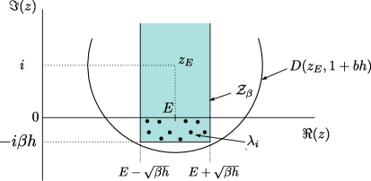
Figure 9: The objective is to bound from above the number of eigenvalues $\lambda_{i}$ in the domain $\mathcal{Z}_{\beta}$. For that purpose, we will bound the number of resonances in the disk of radius $1+bh$ and center $z_{E}=E+i$.

4.5.3 Main idea of the proof

Before giving the details of the proof we give here the main arguments that we will use in order to prove (48).

Let us consider the following complex valued function $\widetilde{p}\left(x,\xi\right)\in C^{\infty}\left(T^{*}X\right)$ made from the first two leading terms of the symbol (60):

$$\widetilde{p}\left(x,\xi\right):=V\left(\xi\right)+ih\mathbf{X}\left(G_{m}\right).$$ (63)

Let $E\in\mathbb{R}\backslash\left\{0\right\}$ and $h\ll 1$. We define the spectral domain $\mathcal{Z}\subset\mathbb{C}$:

$$\mathcal{Z}:=\left\{z\in\mathbb{C},\quad\left|\Re\left(z\right)-E\right|\leq\sqrt{C_{m}h},\quad\Im\left(z\right)\geq-C_{m}h\right\}.$$

See Figure 9. Let

$$\mathcal{V}_{\mathcal{Z}}:=\left\{\left(x,\xi\right)\in T^{*}X,\quad\widetilde{p}\left(x,\xi\right)\in\mathcal{Z}\right\}.$$ (64)

We have from (61)

$$\left(x,\xi\right)\in\mathcal{V}_{\mathcal{Z}}\Leftrightarrow\begin{cases}\left|V\left(\xi\right)-E\right|^{2}\leq C_{m}h\\ h\mathbf{X}\left(G_{m}\right)\left(x,\xi\right)\geq-C_{m}h\end{cases}\Rightarrow\begin{cases}\left(x,\xi\right)&\in\mathbf{\Sigma}_{E\pm\sqrt{C_{m}h}}\\ \left(x,\xi\right)&\in\left(D_{R}\cup\widetilde{N}_{0}\right)\end{cases},$$ (65)

where $\mathbf{\Sigma}_{E\pm\sqrt{C_{m}h}}:=\left(\bigcup_{\left|E^{\prime}-E\right|\leq\sqrt{C_{m}h}}\Sigma_{E^{\prime}}\right)$ is a union a energy shells (28). We deduce that the symplectic volume of $\mathcal{V}_{\mathcal{Z}}$ is

$$\mathrm{Vol}\left(\mathcal{V}_{\mathcal{Z}}\right)\leq C\,\mathrm{Vol}\left(X\right)\mathrm{Vol}\left(\widetilde{N}_{0}\right)\sqrt{h},$$ (66)

with some constant $C>0$. See Figure 10.

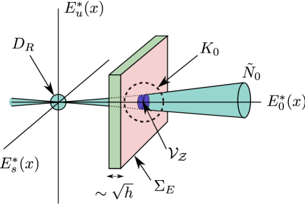
Figure 10: Picture in $T_{x}^{*}X$ with $x\in X$, of the volume $\mathcal{V}_{Z}$ which supports micro-locally the eigenvalues $\lambda_{i}\in\mathcal{Z}$ of figure 9.

Using the “max-min formula” and “Weyl inequalities” we will obtain an upper bound for the number of eigenvalues (in a smaller domain $\mathcal{Z}_{\beta}\subset\mathcal{Z}$) in terms of this upper bound:

$$\sharp\left\{\lambda_{i}\in\mathcal{Z}_{\beta}\right\}\leq\frac{C_{m}\mathrm{Vol}\left(\mathcal{V}_{\mathcal{Z}}\right)}{h^{n}}=C_{m}C\,\mathrm{Vol}\left(X\right)\mathrm{Vol}\left(\widetilde{N}_{0}\right)h^{1/2-n},\qquad\beta<\frac{1}{4}C_{m},$$

with

$$\mathcal{Z}_{\beta}:=\left\{\lambda\in\mathbb{C},\quad\left|\Re\left(\lambda\right)-E\right|\leq\sqrt{\beta h},\quad\Im\left(\lambda\right)\geq-\beta h\right\}.$$ (67)

Using $C_{m}$ arbitrarily large and that $\mathrm{Vol}\left(\widetilde{N}_{0}\right)$ is independently arbitrarily small, from Eq.(62), we deduce that

$$\sharp\left\{\lambda_{i}\in\mathcal{Z}_{\beta}\right\}\leq o\left(h^{1/2-n}\right),$$

which is precisely (48) with $\alpha=1/h$.

The proof below follows these ideas but is not so simple because $P\left(x,\xi\right)$ in Eq.(60) is a symbol and not simply a function (symbols belongs to a non commutative algebra of star product) and because the term $h\mathbf{X}\left(G_{m}\right)$ is subprincipal. We will have to decompose the phase space $T^{*}X$ in different parts in order to separate the different contributions as in (65). Another technical difficulty is that the width of the volume $\mathcal{V}_{\mathcal{Z}}$ is of order $\sqrt{h}$. We will use FBI quantization which is convenient for a sharp control on phase space at the scale $\sqrt{h}$.

4.5.4 Proof of Theorem 15

We present in reverse order the main steps we will follow in the proof.

Steps of the proof:

• Our purpose is to bound the cardinal of the spectrum $\sigma\left(\widehat{P}\right)$ of the operator $\widehat{P}$ in the rectangular domain $\mathcal{Z}_{\beta}$ given by (67). But as suggested by figure 9 and confirmed by Lemma 23 below, it suffices to bound the number of eigenvalues of $\widehat{P}$ in the disk

  $$D\left(z_{E},1+bh\right):=\left\{z\in\mathbb{C},\quad\left|z-z_{E}\right|\leq\left(1+bh\right)\right\},\qquad b>0,$$

  with radius $\left(1+bh\right)$ and center:

  $$z_{E}:=E+i\in\mathbb{C}.$$

  Lemma 23.

  If $b>2\beta$ and $h$ small enough then $$\left(\sigma\left(\widehat{P}\right)\bigcap\mathcal{Z}_{\beta}\right)\subset D\left(z_{E},1+bh\right).$$

  Proof.

  We know from a remark after Theorem 12 that $z\in\sigma\left(\widehat{P}\right)\Rightarrow\Im\left(z\right)\leq 0$. Also, Pythagora’s Theorem in the corner of $\mathcal{Z}$ gives the condition $\left(1+bh\right)^{2}>\left(1+\beta h\right)^{2}+\left(\sqrt{\beta h}\right)^{2}$ which is fulfilled if $b>2\beta$ and $h$ small enough. ∎

• In order to bound the number of eigenvalues of $\widehat{P}$ in the disk $D\left(z_{E},1+bh\right)$, we will use Weyl inequalities in Corollary 28 page 28 and a bound for the number of small singular values of the operator $\left(\widehat{P}-z_{E}\right)$ (i.e. eigenvalues of $\left(\widehat{P}-z_{E}\right)^{*}\left(\widehat{P}-z_{E}\right)$) obtained in Lemma 27.

• In order to get this bound on singular values, we will bound from below the expressions $\left\|\left(\widehat{P}-z_{E}\right)u\right\|^{2}=\left(\left(\widehat{P}-z_{E}\right)^{*}\left(\widehat{P}-z_{E}\right)u|u\right)$. From symbolic calculus (see footnote 10 page 10) we can compute the symbol of this operator and get:

  $$\left(\widehat{P}-z_{E}\right)^{*}\left(\widehat{P}-z_{E}\right) =\mathrm{Op}\left(\left|V\left(\xi\right)-E\right|^{2}+\left|1-h\mathbf{X}\left(G_{m}\right)\right|^{2}+\mathcal{O}\left(hS^{1}\right)+\mathcal{O}_{m}\left(h^{2}S^{+0}\right)\right)$$ (68)

  $$=\mathrm{Op}\left(\left|V\left(\xi\right)-E\right|^{2}+1-2h\mathbf{X}\left(G_{m}\right)+\mathcal{O}\left(hS^{1}\right)+\mathcal{O}_{m}\left(h^{2}S^{+0}\right)\right).$$

  However it is not possible to deduce directly estimates from this symbol because for large $\left|\xi\right|$ the remainders $\mathcal{O}\left(hS^{1}\right)$ and $\mathcal{O}_{m}\left(h^{2}S^{+0}\right)$ may dominate the important term $2h\mathbf{X}\left(G_{m}\right)\in hS^{+0}$. Therefore we first have to perform a partition of unity on phase space.

Partition of unity on phase space:

Let $K_{0}\subset T^{*}X$ be a compact subset (independent of $h$) such that $\mathcal{V}_{\mathcal{Z}}\subset K_{0}$ with $\mathcal{V}_{\mathcal{Z}}$ defined in (64). See figure 10. Lemma 31 page 31 associates a “quadratic partition of unity of PDO” to the compact set $K_{0}$:

$$\boxed{\widehat{\chi}_{0}^{2}+\widehat{\chi}_{1}^{2}=1+\mathrm{Op}\left(h^{\infty}S^{-\infty}\right)}$$ (69)

with self-adjoint operators $\widehat{\chi}_{0},\widehat{\chi}_{1}$ with symbols $\chi_{0}\in S^{-\infty}$, $\chi_{1}\in S^{0}$. On the compact set $K_{0}$, $\chi_{0}=1+\mathcal{O}\left(h^{\infty}\right)$, $\chi_{1}=\mathcal{O}\left(h^{\infty}\right)$.

Then from Lemma 32 page 32 called “IMS localization formula” we have: for every $u\in L^{2}\left(X\right)$,

$$\boxed{\left\|\left(\widehat{P}-z_{E}\right)u\right\|^{2}=\left\|\left(\widehat{P}-z_{E}\right)\widehat{\chi}_{0}u\right\|^{2}+\left\|\left(\widehat{P}-z_{E}\right)\widehat{\chi}_{1}u\right\|^{2}+\mathcal{O}\left(h^{2}\right)\left\|u\right\|^{2}.}$$ (70)

We will now study the different terms of (70) separately.

Informal remark:

In order to show that the Lemma 24 below is expected, let us give an informal remark (non necessary for the proof). Using the function $\widetilde{p}\left(x,\xi\right):=V\left(\xi\right)+ih\mathbf{X}\left(G_{m}\right)$, as in (63), which is the dominant term of the symbol $P\left(x,\xi\right)$, we write:

$$\left|\widetilde{p}\left(x,\xi\right)-z_{E}\right|^{2} =\left|V\left(\xi\right)-E\right|^{2}+\left|1-h\mathbf{X}\left(G_{m}\right)\right|^{2}$$ (71)

$$=\left|V\left(\xi\right)-E\right|^{2}+1-2h\mathbf{X}\left(G_{m}\right)+\mathcal{O}\left(h^{2}S^{+0}\right).$$ (72)

If $\left(x,\xi\right)\notin K_{0}$ there are two cases, according to (61):

1. Either $\mathbf{X}\left(G_{m}\right)\left(x,\xi\right)\leq-C_{m}$ , therefore:

   $$\left|\widetilde{p}\left(x,\xi\right)-z_{E}\right|^{2}\geq 1+2hC_{m}.$$

2. or $\left|V\left(\xi\right)-E\right|^{2}\geq C_{0}>0$ and $\mathbf{X}\left(G_{m}\right)\leq\mathcal{O}\left(1\right)$ from (61). Therefore

   $$\left|\widetilde{p}\left(x,\xi\right)-z_{E}\right|^{2}\geq 1+C_{0}+\mathcal{O}\left(h\right).$$

In both cases we have

$$\left(x,\xi\right)\notin K_{0}\Rightarrow\left|\widetilde{p}\left(x,\xi\right)-z_{E}\right|^{2}\geq 1+2hC_{m}.$$ (73)

Since $\chi_{1}$ is negligible on $K_{0}$, the following Lemma 24 is not surprising in the light of property (73). It gives a lower bound for the second term in the right side of (70).

Lemma 24.

For every $u\in L^{2}\left(X\right)$, $$\left\|\left(\widehat{P}-z_{E}\right)\widehat{\chi}_{1}u\right\|^{2}\geq\left(1+2h\left(C_{m}-C\right)\right)\left\|\widehat{\chi}_{1}u\right\|^{2}-\mathcal{O}\left(h^{\infty}\right)\left\|u\right\|^{2}.$$ (74)

Proof.

In order to prove (74) we have to consider a partition of unity in order to take into account two contributions as in the discussion after (71). Let $\Psi_{0}\in S^{0}$ which has its support inside the region where $\chi_{1}=1$ and we set $\Psi_{0}=1$ away from a conical neighborhood of the energy shell $\Sigma_{E}$, Eq.(28), which is the characteristic set $V\left(\xi\right)-E=0$. See figure 11.

Figure 11: Picture in $T_{x}^{*}X$ with $x\in X$, which shows the partition of unity of phase space used in the proof of Lemma 24. The support of $\chi_{1}$ is outside the set $K_{0}$.

Since $\left(V\left(\xi\right)-E\right)$ is the principal symbol of $\left(P\left(x,\xi\right)-E\right)\in S^{1}$ and is non vanishing on the support of $\Psi_{0}$, there exists $\widehat{Q}\in\mathrm{Op}\left(S^{-1}\right)$ such that

$$\widehat{Q}\left(\widehat{P}-E\right)=\widehat{\Psi}_{0}+\widehat{R},\qquad\widehat{R}\in\mathrm{Op}\left(h^{\infty}S^{-\infty}\right).$$

Since $\widehat{Q}$ is continuous in $L^{2}\left(X\right)$, there exists $C_{0}>0$ such that for every $v\in L^{2}\left(X\right)$, $\left\|v\right\|^{2}\geq\frac{1}{C_{0}}\left\|\widehat{Q}v\right\|^{2}$, hence for every $u\in L^{2}\left(X\right)$

$$\left\|\left(\widehat{P}-E\right)\widehat{\chi}_{1}u\right\|^{2} \geq\frac{1}{C_{0}}\left\|\widehat{Q}\left(\widehat{P}-E\right)\widehat{\chi}_{1}u\right\|^{2}=\frac{1}{C_{0}}\left\|\left(\widehat{\Psi}_{0}+\widehat{R}\right)\widehat{\chi}_{1}u\right\|^{2}$$ (75)

$$\geq\frac{1}{2C_{0}}\left\|\widehat{\Psi}_{0}\widehat{\chi}_{1}u\right\|^{2}-\mathcal{O}\left(h^{\infty}\right)\left\|u\right\|^{2}.$$

Writing $\widehat{P}=\widehat{P}_{1}+i\widehat{P}_{2}$ with $\widehat{P}_{i}$ self-adjoint, we have

$$\left\|\left(\widehat{P}-z_{E}\right)\widehat{\chi}_{1}u\right\|^{2} =\left(\left(\left(\widehat{P}-E\right)^{*}+i\right)\left(\left(\widehat{P}-E\right)-i\right)\widehat{\chi}_{1}u|\widehat{\chi}_{1}u\right)$$ (76)

$$=\left\|\left(\widehat{P}-E\right)\widehat{\chi}_{1}u\right\|^{2}+\left\|\widehat{\chi}_{1}u\right\|^{2}-\left(2\widehat{P}_{2}\widehat{\chi}_{1}u|\widehat{\chi}_{1}u\right).$$

Using (75) in (76) we get for every $a>0$:

$$\left\|\left(\widehat{P}-z_{E}\right)\widehat{\chi}_{1}u\right\|^{2} =\left(1-ah\right)\left\|\left(\widehat{P}-E\right)\widehat{\chi}_{1}u\right\|^{2}+ah\left\|\left(\widehat{P}-E\right)\widehat{\chi}_{1}u\right\|^{2}+\left\|\widehat{\chi}_{1}u\right\|^{2}$$ (77)

$$\qquad-\left(2\widehat{P}_{2}\widehat{\chi}_{1}u|\widehat{\chi}_{1}u\right)$$

$$\geq\left(1-ah\right)\left\|\left(\widehat{P}-E\right)\widehat{\chi}_{1}u\right\|^{2}+\left\|\widehat{\chi}_{1}u\right\|^{2}-\left(2\widehat{P}_{2}\widehat{\chi}_{1}u|\widehat{\chi}_{1}u\right)$$

$$\qquad+\frac{ah}{2C_{0}}\left\|\widehat{\Psi}_{0}\widehat{\chi}_{1}u\right\|^{2}-\mathcal{O}\left(h^{\infty}\right)\left\|u\right\|^{2}$$

$$=\left(1-ah\right)\left\|\left(\widehat{P}-E\right)\widehat{\chi}_{1}u\right\|^{2}+\left\|\widehat{\chi}_{1}u\right\|^{2}$$

$$\qquad+\left(\left(-2\widehat{P}_{2}+\frac{ah}{2C_{0}}\widehat{\Psi}_{0}^{*}\widehat{\Psi}_{0}\right)\widehat{\chi}_{1}u|\widehat{\chi}_{1}u\right)-\mathcal{O}\left(h^{\infty}\right)\left\|u\right\|^{2}.$$

Recall from (60) that

$$\widehat{P}_{2}=\mathrm{Op}\left(h\mathbf{X}\left(G_{m}\right)+\mathcal{O}\left(hS^{0}\right)\right)\in\mathrm{Op}\left(hS^{+0}\right).$$

Therefore

$$\left(-2\widehat{P}_{2}+\frac{ah}{2C_{0}}\widehat{\Psi}_{0}^{*}\widehat{\Psi}_{0}\right)\in\mathrm{Op}\left(hS^{+0}\right).$$

Assume $a\geq 4C_{0}\left(C_{m}-C\right)$. Then from (61) and the hypothesis on $\Psi_{0}$, for every $\left(x,\xi\right)\in\mathrm{supp}\left(\chi_{1}\right)$ we have

$$\left(-2P_{2}+\frac{ah}{2C_{0}}\Psi_{0}^{*}\Psi_{0}\right)\left(x,\xi\right)\geq\min\left(2h\left(C_{m}-C\right),\frac{ah}{2C_{0}}\right)\geq 2h\left(C_{m}-C\right).$$

We can add a symbol $\Psi_{1}\in S^{0}$ positive, which vanishes on $\mathrm{supp}\left(\chi_{1}\right)$ so that $\widehat{\Psi}_{1}\widehat{\chi}_{1}\in\mathrm{Op}\left(h^{\infty}S^{-\infty}\right)$ and such that for every $\left(x,\xi\right)\in T^{*}X$ we have

$$\left(-2P_{2}+\frac{ah}{2C_{0}}\Psi_{0}^{*}\Psi_{0}+\Psi_{1}\right)\left(x,\xi\right)\geq\min\left(2h\left(C_{m}-C\right),\frac{ah}{2C_{0}}\right)\geq 2h\left(C_{m}-C\right).$$

The semiclassical sharp Gårding inequality implies that:

$$\forall u\in L^{2}\left(X\right),\quad\left(\left(-2\widehat{P}_{2}+\frac{ah}{2C_{0}}\widehat{\Psi}_{0}^{*}\widehat{\Psi}_{0}\right)\widehat{\chi}_{1}u|\widehat{\chi}_{1}u\right)\geq \left(2h\left(C_{m}-C\right)-\mathcal{O}\left(h^{2}\right)\right)\left\|\widehat{\chi}_{1}u\right\|^{2}$$

$$-\mathcal{O}\left(h^{\infty}\right)\left\|u\right\|^{2},$$

where the remainder term $\mathcal{O}\left(h^{\infty}\right)\left\|u\right\|^{2}$ comes from $\left(\widehat{\Psi}_{1}\widehat{\chi}_{1}u|\widehat{\chi}_{1}u\right)$. With (77) we get:

$$\left\|\left(\widehat{P}-z_{E}\right)\widehat{\chi}_{1}u\right\|^{2} \geq\left(1-ah\right)\left\|\left(\widehat{P}-E\right)\widehat{\chi}_{1}u\right\|^{2}+\left\|\widehat{\chi}_{1}u\right\|^{2}$$

$$\qquad+\left(2h\left(C_{m}-C\right)-\mathcal{O}\left(h^{2}\right)\right)\left\|\widehat{\chi}_{1}u\right\|^{2}-\mathcal{O}\left(h^{\infty}\right)\left\|u\right\|^{2}$$

$$\geq\left(1+2h\left(C_{m}-C\right)-\mathcal{O}\left(h^{2}\right)\right)\left\|\widehat{\chi}_{1}u\right\|^{2}-\mathcal{O}\left(h^{\infty}\right)\left\|u\right\|^{2}.$$

The term $\mathcal{O}\left(h^{2}\right)\left\|\widehat{\chi}_{1}u\right\|^{2}$ can be absorbed in the constant $C$. ∎

Lemma 25.

There exists a family of trace class operators $\widehat{B}_{h}$ (depending on $h$) such that $$\left\|\widehat{B}_{h}\right\|_{\mathrm{Tr}}\leq\mathcal{O}\left(1\right)C_{m}\mathrm{Vol}\left(\widetilde{N}_{0}\right)h^{1/2-n},\qquad\widehat{B}_{h}\geq 0,$$ (78) (where the constant $\mathcal{O}\left(1\right)$ does not depend on the escape function $m$) and for every $u\in L^{2}\left(X\right)$, $$\left\|\left(\widehat{P}-z_{E}\right)\widehat{\chi}_{0}u\right\|^{2}+\left(h\widehat{B}_{h}u|u\right)\geq\left(1+2h\left(C_{m}-\mathcal{O}\left(1\right)\right)\right)\left\|\widehat{\chi}_{0}u\right\|^{2}-\mathcal{O}\left(h^{\infty}\right)\left\|u\right\|^{2},$$ (79) and $$\left\|\left(\widehat{P}-z_{E}\right)\widehat{\chi}_{0}u\right\|^{2}\geq\left(1-\mathcal{O}\left(h\right)\right)\left\|\widehat{\chi}_{0}u\right\|^{2}-\mathcal{O}\left(h^{\infty}\right)\left\|u\right\|^{2},$$ (80) where the term $\mathcal{O}\left(h\right)$ does not depend on $m$.

Remarks

Lemma 25 concerns the first term of the right hand side of (70). In order to obtain (79), which is similar to (74), it has been necessary to add a new term which involves a trace class operator $\widehat{B}_{h}$. Its role is to “hide” the domain $\mathcal{V}_{\mathcal{Z}}$ (65). Eq.(80) shows that without this term the lower bound is smaller.

Proof.

The construction is based on ideas around Anti-Wick quantization, Berezin quantization, FBI transforms, Bargmann-Segal transforms, Gabor frames and Toeplitz operators, see e.g. [26]. We review some definitions in Appendix A.4 page A.4. We will use the following two properties for an operator obtained by Toeplitz quantization of a symbol $A\left(x,\xi;h\right)$. Let

$$\widehat{A}:=\mathrm{Op}_{T}\left(A\right):=\int A\left(x,\xi;h\right)\widehat{\pi}_{\alpha}d\alpha.$$

Gårding’s inequality writes

$$A\left(x,\xi\right)\geq 0\Rightarrow\left(\widehat{A}u|u\right)\geq 0+\mathcal{O}\left(h^{\infty}\right)\left\|u\right\|^{2},$$ (81)

also

$$\mathrm{Tr}\left(\widehat{A}\right)=\frac{\mathcal{O}\left(1\right)}{h^{n}}\int A\left(x,\xi\right)dxd\xi+\mathcal{O}\left(h^{\infty}\right),$$ (82)

and

$$\left(\forall\left(x,\xi\right),\quad A\left(x,\xi\right)\geq 0\right)\quad\Rightarrow\quad\left\|\widehat{A}\right\|_{\mathrm{Tr}}=\mathrm{Tr}\left(\widehat{A}\right)+\mathcal{O}\left(h^{\infty}\right).$$ (83)

From (68) we have

$$\widehat{\chi}_{0}\left(\widehat{P}-z_{E}\right)^{*}\left(\widehat{P}-z_{E}\right)\widehat{\chi}_{0}=\widehat{\chi}_{0}\widehat{S}\widehat{\chi}_{0}+\widehat{R},$$ (84)

with $\widehat{R}\in\mathrm{Op}\left(h^{\infty}S^{-\infty}\right)$ and

$$\widehat{S}=\mathrm{Op}_{T}\left(S\right),$$

with the Toeplitz symbol

$$S\left(x,\xi;h\right)=\left|V\left(\xi\right)-E\right|^{2}+1-2h\mathbf{X}\left(G_{m}\right)\left(x,\xi\right)+\mathcal{O}\left(hS^{-\infty}\right)+\mathcal{O}_{m}\left(h^{2}S^{-\infty}\right)$$

(the remainders are in $S^{-\infty}$ since $\chi_{0}$ has compact support in (84). Since $\mathbf{X}\left(G_{m}\right)\leq 0$ from (61), we deduce (80) using Gårding’s inequality (81).

In order to improve this lower bound and get (79), let $B_{h}\in C_{0}^{\infty}\left(T^{*}X\right)$ such that $\forall\left(x,\xi\right),\,B_{h}\left(x,\xi\right)\geq 0$ and

$$\left(x,\xi\right)\in\mathcal{V}_{\mathcal{Z}}\Rightarrow B_{h}\left(x,\xi\right)\geq 2C_{m}.$$ (85)

Notice that from (66) $B_{h}$ can be chosen such that

$$\int_{T^{*}X}B_{h}\left(x,\xi\right)dxd\xi\leq\mathcal{O}\left(1\right)C_{m}\mathrm{Vol}\left(\mathcal{V}_{\mathcal{Z}}\right)=\mathcal{O}\left(1\right)C_{m}\mathrm{Vol}\left(X\right)\mathrm{Vol}\left(\widetilde{N}_{0}\right)\sqrt{h}.$$ (86)

From (83), (82) and (86) we deduce (78). Recall that from (65) we have

$$\left(x,\xi\right)\notin\mathcal{V}_{\mathcal{Z}}\Rightarrow\left|V\left(\xi\right)-E\right|^{2}\geq hC_{m}\mbox{ or }-h\mathbf{X}\left(G_{m}\right)\geq hC_{m}.$$

Therefore in view of (85) for every $\left(x,\xi\right)\in T^{*}X$ we have

$$S\left(x,\xi;h\right)+hB_{h}\left(x,\xi\right) =\left|V\left(\xi\right)-E\right|^{2}+1-2h\mathbf{X}\left(G_{m}\right)+hB_{h}\left(x,\xi\right)$$

$$\qquad+\mathcal{O}\left(hS^{-\infty}\right)+\mathcal{O}_{m}\left(h^{2}S^{-\infty}\right)$$

$$\geq 1+2hC_{m}+\mathcal{O}\left(hS^{-\infty}\right)+\mathcal{O}_{m}\left(h^{2}S^{-\infty}\right).$$

Let $\widehat{B}_{h}:=\mathrm{Op}_{T}\left(B_{h}\right)$. After multiplying both sides by $\widehat{\chi}_{0}$, using $\widehat{\chi}_{0}\widehat{B}_{h}\widehat{\chi}_{0}=\widehat{B}_{h}+\mathrm{Op}\left(h^{\infty}S^{-\infty}\right)$ and Gårding’s inequality we deduce that

$$\forall u\in L^{2}\left(X\right),\quad\left(\widehat{\chi}_{0}\widehat{S}\widehat{\chi}_{0}u|u\right)+\left(h\widehat{B}_{h}u|u\right)\geq\left(\left(\widehat{\chi}_{0}\left(1+2h\left(C_{m}-\mathcal{O}\left(1\right)\right)\right)\widehat{\chi}_{0}\right)u|u\right)+\mathcal{O}\left(h^{\infty}\right)\left\|u\right\|^{2}.$$

Replacing the first term by (84) this gives (79). ∎

Corollary 26.

Eq. (70) with (74), (79), (69) gives: $$\forall u\in L^{2}\left(X\right),\qquad\left\|\left(\widehat{P}-z_{E}\right)u\right\|^{2}+\left(h\widehat{B}_{h}u|u\right)\geq\left(1+2\left(C_{m}-\mathcal{O}\left(1\right)\right)h\right)\left\|u\right\|^{2},$$ (87) where $\mathcal{O}\left(1\right)$ does not depend on $m$. Using (80) instead we get $$\forall u\in L^{2}\left(X\right),\qquad\left\|\left(\widehat{P}-z_{E}\right)u\right\|^{2}\geq\left(1-\mathcal{O}\left(h\right)\right)\left\|u\right\|^{2}.$$ (88)

Let us show that these last relations imply an upper bound for the number of eigenvalues of the operator $\left(\widehat{P}-z_{E}\right)^{*}\left(\widehat{P}-z_{E}\right)$ smaller than $\left(1+2\left(C_{m}-\mathcal{O}\left(1\right)\right)h\right)$.

Lemma 27.

Let $s_{1}\leq s_{2}\leq\ldots$ be the singular values $\left(\widehat{P}-z_{E}\right)$ sorted from below. More precisely, $s_{1}^{2}\leq s_{2}^{2}\leq\ldots$ are the eigenvalues of the positive self-adjoint operator $\widehat{A}:=\left(\widehat{P}-z_{E}\right)^{*}\left(\widehat{P}-z_{E}\right)$ below the infimum of the essential spectrum of $\widehat{A}$, possibly completed with an infinite repetition of that infimum if there are only finitely many such eigenvalues. Then the first eigenvalue is $$s_{1}\geq 1-\mathcal{O}\left(h\right)$$ (89) and $$\mbox{if }j>\mathcal{O}\left(1\right)C_{m}\mathrm{Vol}\left(\widetilde{N}_{0}\right)h^{\frac{1}{2}-n}\mbox{ then }s_{j}\geq 1+\left(C_{m}-\mathcal{O}\left(1\right)\right)h.$$ (90) In other words the number of singular values of $\left(\widehat{P}-z_{E}\right)$ below $1+\left(C_{m}-\mathcal{O}\left(1\right)\right)h$ is $\mathcal{O}\left(1\right)C_{m}\mathrm{Vol}\left(\widetilde{N}_{0}\right)h^{\frac{1}{2}-n}$.

Proof.

Eq.(89) is a direct consequence of (88). We use the “max-min formula” for self-adjoint operators [38, p.78] and Eq.(87). Put $\lambda_{m}:=C_{m}-\mathcal{O}\left(1\right)$. We have for every $j$

$$s_{j}^{2} =\max_{U\subseteq L^{2}\left(X\right),\,\mathrm{codim}\left(U\right)\leq j-1}\quad\min_{u\in U,\left\|u\right\|=1}\left(u,\widehat{A}u\right)$$

$$\geq 1+2\lambda_{m}h+\max_{U\subseteq L^{2}\left(X\right),\,\mathrm{codim}\left(U\right)\leq j-1}\quad\min_{u\in U,\left\|u\right\|=1}\left(-\left(h\widehat{B}_{h}u|u\right)\right)$$

$$=1+2\lambda_{m}h-h\min_{U\subseteq L^{2}\left(X\right),\,\mathrm{codim}\left(U\right)\leq j-1}\quad\max_{u\in U,\left\|u\right\|=1}\left(\left(\widehat{B}_{h}u|u\right)\right)$$

$$=1+2\lambda_{m}h-hb_{j},$$

where $U$ varies in the set of closed subspaces of $L^{2}\left(X\right)$ and $b_{1}\geq b_{2}\geq\ldots$ denote the eigenvalues of $\widehat{B}_{h}$ (possibly completed with an infinite repetition of $0$ if there are only finitely many such eigenvalues). We have

$$\left\|\widehat{B}_{h}\right\|_{\mathrm{Tr}}=\mathrm{Tr}\left(\widehat{B}_{h}\right)=b_{1}+b_{2}+\ldots$$

Eq.(78) implies that for every $\varepsilon_{0}>0$, if $b_{j}\geq\varepsilon_{0}$ then $j\varepsilon_{0}\leq\mathrm{Tr}\left(\widehat{B}_{h}\right)\leq\mathcal{O}\left(1\right)C_{m}\mathrm{Vol}\left(\widetilde{N}_{0}\right)h^{\frac{1}{2}-n}$ then $j\leq\frac{1}{\varepsilon_{0}}\mathcal{O}\left(1\right)C_{m}\mathrm{Vol}\left(\widetilde{N}_{0}\right)h^{\frac{1}{2}-n}$. Equivalently if $j>\frac{1}{\varepsilon_{0}}\mathcal{O}\left(1\right)C_{m}\mathrm{Vol}\left(\widetilde{N}_{0}\right)$ then $b_{j}<\varepsilon_{0}$ and $s_{j}^{2}\geq 1+2\lambda_{m}h-hb_{j}\geq 1+2\left(\lambda_{m}-\varepsilon_{0}\right)h$. Taking the square root we get (90). ∎

We deduce now an upper bound for the number of eigenvalues of $\widehat{P}$.

Corollary 28.

We have $$\sharp\left\{\sigma\left(\widehat{P}\right)\cap D\left(z_{E},1+\frac{C_{m}}{2}h\right)\right\}\leq\mathcal{O}\left(1\right)C_{m}\mathrm{Vol}\left(\widetilde{N}_{0}\right)h^{\frac{1}{2}-n}.$$ (91)

Proof.

Let $\lambda_{1},\lambda_{2},\lambda_{3}\ldots$ denote the eigenvalues of $\widehat{P}$ sorted such that $j\rightarrow\left|\lambda_{j}-z_{E}\right|$ is increasing. The Weyl inequalities (see [42, (a.8) p.38] for a proof) give

$$\prod_{j=1}^{N}s_{j}\leq\prod_{j=1}^{N}\left|\lambda_{j}-z_{E}\right|,\qquad\forall N,$$ (92)

where $\left(s_{j}\right)_{j}$ are the singular values defined in Lemma 27 above. Let

$$\widetilde{N}:=\sharp\left\{\lambda_{j}:\quad\left|\lambda_{j}-z_{E}\right|\leq 1+\frac{C_{m}}{2}h\right\}=\sharp\left\{\sigma\left(P\right)\cap D\left(z_{E},1+\frac{C_{m}}{2}h\right)\right\}$$

and let

$$\widetilde{M}:=\mathcal{O}\left(1\right)C_{m}\mathrm{Vol}\left(\widetilde{N}_{0}\right)h^{\frac{1}{2}-n}$$

be the factor which appears in (90). We want to show the bound:

$$\widetilde{N}\leq\left(2+\mathcal{O}\left(\frac{1}{C_{m}}\right)\right)\widetilde{M}$$ (93)

for $C_{m}\gg 1$.

If $\widetilde{N}\leq\widetilde{M}$ then (93) is true. Conversely let us suppose that $\widetilde{N}\geq\widetilde{M}$. Using (92) we have

$$\left(\prod_{j=1}^{\widetilde{M}}s_{j}\right)\left(\prod_{j=\widetilde{M}}^{\widetilde{N}}s_{j}\right)\leq\left(1+\frac{C_{m}}{2}h\right)^{\widetilde{N}}.$$

Then using (89) and (90) we have

$$\left(1-\mathcal{O}\left(h\right)\right)^{\widetilde{M}}\left(1+\left(C_{m}-\mathcal{O}\left(1\right)\right)h\right)^{\widetilde{N}-\widetilde{M}}\leq\left(1+\frac{C_{m}}{2}h\right)^{\widetilde{N}}.$$

We take the logarithm and since $h\ll 1$ we get:

$$-\widetilde{M}\mathcal{O}\left(h\right)+\left(\widetilde{N}-\widetilde{M}\right)\left(C_{m}-\mathcal{O}\left(1\right)\right)h\leq\widetilde{N}\frac{C_{m}}{2}h$$

$$\Leftrightarrow\widetilde{N}\left(\frac{C_{m}}{2}-\mathcal{O}\left(1\right)\right)\leq\widetilde{M}\left(C_{m}+\mathcal{O}\left(1\right)\right).$$

Now since $C_{m}\gg 1$,

$$\Leftrightarrow\widetilde{N}\leq\widetilde{M}\frac{\left(1+\mathcal{O}\left(\frac{1}{C_{m}}\right)\right)}{\left(\frac{1}{2}+\mathcal{O}\left(\frac{1}{C_{m}}\right)\right)}=\widetilde{M}\left(2+\mathcal{O}\left(\frac{1}{C_{m}}\right)\right),$$

so we have obtained (93). This implies (91). ∎

From Lemma 23 with $b=\frac{C_{m}}{2}$ and $\beta=\frac{C_{m}}{4}$ we deduce that the upper bound (91) implies an upper bound:

$$\sharp\left\{\lambda_{i}\in\sigma\left(\widehat{P}\right),\quad\left|\Re\left(\lambda_{i}-E\right)\right|\leq\sqrt{\frac{C_{m}}{4}h},\quad\Im\left(\lambda_{i}\right)\geq-\frac{C_{m}}{4}h\right\}=\mathcal{O}\left(1\right)C_{m}\mathrm{Vol}\left(\widetilde{N}_{0}\right)h^{\frac{1}{2}-n}.$$

We take $\alpha=\frac{1}{h}\gg 1$ and return to the original spectral variable $z=\frac{z_{h}}{h}=\alpha z_{h}$ after the scaling (59). From (62) we can choose the escape function $m$ such that $C_{m}\gg 1$ is arbitrarily large and $\mathrm{Vol}\left(\widetilde{N}_{0}\right)<o\left(\frac{1}{C_{m}}\right)$ is arbitrarily small so that $\mathcal{O}\left(1\right)C_{m}\mathrm{Vol}\left(\widetilde{N}_{0}\right)h^{\frac{1}{2}-n}=o\left(h^{\frac{1}{2}-n}\right)$. Since the spectrum does not depend on the escape function $m$, we get (48). We have finished the proof of Theorem 15.

Appendix A Some results in operator theory

A.1 On minimal and maximal extensions

We show here that the pseudodifferential operator $\widehat{P}$ defined in Eq.(49), has a unique closed extension on $L^{2}\left(X\right)$. This a well known procedure for the case of elliptic PDO, we refer to [51, chap.13 p.125], and in general this is not true for PDO of order 2. The fact that $P$ has order 1 (since it is defined from a vector field on $X$) is therefore important.

The domain of the minimal closed extension $\widehat{P}_{min}$ of the operator $\widehat{P}$ with domain $C^{\infty}\left(X\right)$ is

$$\mathcal{D}_{min}:=\left\{u\in L^{2}\left(X\right),\quad u_{j}\in C^{\infty}\left(X\right)\rightarrow u\mbox{ in }L^{2}\left(X\right)\mbox{ and }\widehat{P}u_{j}\rightarrow v\in L^{2}\left(X\right)\right\}.$$ (94)

The maximal closed extension $\widehat{P}_{max}$ has domain

$$\mathcal{D}_{max}:=\left\{u\in L^{2}\left(X\right),\quad\widehat{P}u\in L^{2}\left(X\right)\right\}.$$

(Recall that $\widehat{P}$ is defined a priori on $C^{\infty}\left(X\right)$ and $\mathcal{D}^{\prime}\left(X\right)$).

Lemma 29.

For a PDO $\widehat{P}$ of order $1$ (i.e $\widehat{P}\in\mathrm{Op}\left(S^{1}\right)$), the minimal and maximal extensions coincide: $\mathcal{D}\left(\widehat{P}\right):=\mathcal{D}_{min}=\mathcal{D}_{max}$, i.e. there is a unique closed extension of the operator $\widehat{P}$ in $L^{2}\left(X\right)$.

Proof.

$\mathcal{D}_{min}\subset\mathcal{D}_{max}$ is clear. Let us check that $\mathcal{D}_{max}\subset\mathcal{D}_{min}$. Let $u\in\mathcal{D}_{max}$, i.e. $u\in L^{2}\left(X\right)$, $v:=\widehat{P}u\in L^{2}\left(X\right)$. We will construct a sequence $u_{h}\in C^{\infty}\left(X\right)$ with $h\rightarrow 0$, such that $u_{h}\rightarrow u$ in $L^{2}\left(X\right)$ and show that $\widehat{P}u_{h}\rightarrow v$ in $L^{2}$.

Let $\chi:T^{*}X\rightarrow\mathbb{R}^{+}$ be a $C^{\infty}$ function such that $\chi(x,\xi)=1$ for $\left|\xi\right|\leq 1$, and $\chi\left(x,\xi\right)=0$ for $\left|\xi\right|\geq 2$. For $h>0$, let the function $\chi_{h}$ on $T^{*}X$ be defined by $\chi_{h}\left(x,\xi\right)=\chi\left(x,h\xi\right)$. Let the truncation operator be:

$$\widehat{\chi}_{h}:=\mathrm{Op}\left(\chi_{h}\right).$$

Notice that $\widehat{\chi}_{h}$ is a smoothing operator which truncates large components in $\xi$ (larger than $1/h$), $\widehat{\chi}_{h}$ is similar to a convolution in $x$ coordinates.

Let

$$u_{h}:=\widehat{\chi}_{h}u.$$

It is clear that $u_{h}\rightarrow u$ in $L^{2}\left(X\right)$ as $h\rightarrow 0$. We have

$$\widehat{P}u_{h}=\widehat{P}\widehat{\chi}_{h}u=\widehat{\chi}_{h}\widehat{P}u+\left[\widehat{P},\widehat{\chi}_{h}\right]u.$$

The first term converges $\widehat{\chi}_{h}\widehat{P}u\rightarrow v=\widehat{P}u$ as $h\rightarrow 0$. The principal symbol of the PDO $\left[\widehat{P},\widehat{\chi}_{h}\right]$ is

$$\frac{1}{i}\left\{P,\chi_{h}\right\}=\frac{1}{i}\left(\partial_{\xi}P\partial_{x}\chi_{h}-\partial_{x}P\partial_{\xi}\chi_{h}\right).$$

Now we use the fact that $P\in S^{1}$ has order 1. In the first term, $\partial_{\xi}P\in S^{0}$ is bounded (from (3)) and $\partial_{x}\chi_{h}$ is non zero only on a large ring $\frac{1}{h}\leq\left|\xi\right|\leq\frac{2}{h}$. In the second term $\partial_{x}P\in S^{1}$ has order 1 but $\partial_{\xi}\chi_{h}=h\partial_{\xi}\chi\left(x,h\xi\right)$ is non zero on the same large ring and therefore of order $\left(-1\right)$ (since $h\simeq\left|\xi\right|^{-1}$ on the ring). Therefore the PDO $\left[\widehat{P},\widehat{\chi}_{h}\right]$ converges strongly to zero in $L^{2}\left(X\right)$ as $h\rightarrow 0$. Hence $\left[\widehat{P},\widehat{\chi}_{h}\right]u\rightarrow 0$ as $h\rightarrow 0$. We deduce that $\widehat{P}u_{h}\rightarrow v=\widehat{P}u$, and that $u\in\mathcal{D}_{min}$. ∎

A.2 The sharp Gårding inequality

References: [23, p.52] or (100), [32, p.99], [52, p.1157] for a short proof using Toeplitz quantization.

Proposition 30.

If $\widehat{P}$ is a PDO with symbol $P\in S^{\mu}$, $\mu\in\mathbb{R}$, $\Re\left(P\right)\geq 0$ then there exists $C\in\mathbb{R}$ such that $$\forall u\in C^{\infty}\left(X\right),\quad\Re\left(\widehat{P}u|u\right)\geq-C\left\|u\right\|_{H^{\frac{\mu-1}{2}}}^{2}$$ (95) where $\left\|u\right\|_{H^{\mu}}^{2}:=\left(\left\langle\widehat{\xi}\right\rangle^{\mu}u|\left\langle\widehat{\xi}\right\rangle^{\mu}u\right)_{L^{2}\left(X\right)}$ denotes the norm in the Sobolev space $H^{\mu}$.

A.3 Quadratic partition of unity on phase space

As usual in this paper, we denote $\widehat{A}:=\mathrm{Op}_{h}\left(A\right)$ for a symbol $A$.

Lemma 31.

Let $K_{0}\subset T^{*}X$ compact. There exists symbols $\chi_{0}\in S^{-\infty}$ and $\chi_{1}\in S^{0}$ of self-adjoint operators $\widehat{\chi}_{0},\widehat{\chi}_{1}$ such that $$\widehat{\chi}_{0}^{2}+\widehat{\chi}_{1}^{2}=1+\widehat{R}.$$ The symbol $R\in\left(h^{\infty}S^{-\infty}\right)$ is negligible, $\mathrm{supp}\left(\chi_{0}\right)$ is compact and on $K_{0}$, $\chi_{1}\left(x,\xi\right)=\mathcal{O}\left(h^{\infty}\right)$, $\chi_{0}\left(x,\xi\right)=1+\mathcal{O}\left(h^{\infty}\right)$.

Proof.

Let $K_{0}\subset T^{*}X$ be compact. We can find symbols $0\leq\chi_{0}\in C_{0}^{\infty}\left(T^{*}X\right)$ (with compact support) and $0\leq\chi_{1}\in C^{\infty}\left(T^{*}X\right)$ such that

$$\chi_{1}=\begin{cases}0&\mbox{ on }K_{0}\\ 1&\mbox{ for }\left|\xi\right|\gg 1\end{cases}$$

and

$$A:=\chi_{0}^{2}+\chi_{1}^{2}\mbox{ is }\begin{cases}>0&\mbox{ everywhere}\\ =1&\mbox{ for }\left|\xi\right|\gg 1.\end{cases}$$

We replace $\chi_{0},\chi_{1}$ respectively by $\chi_{0}A^{-1/2}$, $\chi_{1}A^{-1/2}$. We obtain $1=\chi_{0}^{2}+\chi_{1}^{2}$.

Let $\widehat{R}:=\widehat{\chi}_{0}^{2}+\widehat{\chi}_{1}^{2}-1$. Then $\widehat{R}\in\mathrm{Op}\left(hS^{-\infty}\right)$. We write $R=hr_{0}\left(x,\xi\right)+h^{2}\ldots$.

We replace $\widehat{\chi}_{j}$, $j=0,1$ by

$$\widehat{\chi}_{j}^{{}^{\prime}}:=\left(1+h\widehat{r}_{0}\right)^{-1/4}\widehat{\chi}_{j}\left(1+h\widehat{r}_{0}\right)^{-1/4}.$$

Which is also self-adjoint. We obtain

$$\widehat{\chi}_{0}^{{}^{\prime}2}+\widehat{\chi}_{1}^{{}^{\prime}2} =\left(1-h\widehat{r}_{0}\right)\widehat{\chi}_{0}^{2}+\left(1-h\widehat{r}_{1}\right)\widehat{\chi}_{1}^{2}+\mathcal{O}\left(\mathrm{Op}\left(h^{2}S^{-\infty}\right)\right)$$

$$=1+\mathcal{O}\left(\mathrm{Op}\left(h^{2}S^{-\infty}\right)\right).$$

If we iterate this algorithm, we obtain the Lemma. ∎

A.3.1 I.M.S. localization formula

The following Lemma is similar to the “I.M.S localization formula” given in [11, p.27]. It uses the quadratic partition of phase space obtained in Lemma 31 above.

Lemma 32.

Suppose that $\widehat{P}\in\mathrm{Op}\left(S^{\mu}\right)$ for some $\mu\in\mathbb{R}$ and that $\left(P-P^{*}\right)\in\mathrm{Op}\left(hS^{\mu}\right)$. Then for every $u\in L^{2}\left(X\right)$, $z\in\mathbb{C}$, $$\left\|\left(\widehat{P}-z\right)u\right\|^{2}=\left\|\left(\widehat{P}-z\right)\widehat{\chi}_{0}u\right\|^{2}+\left\|\left(\widehat{P}-z\right)\widehat{\chi}_{1}u\right\|^{2}+\mathcal{O}\left(h^{2}\right)\left\|u\right\|^{2}.$$ (96)

Proof.

For simplicity, we suppose $z=i\beta$ with $\beta\in\mathbb{R}$, i.e. $\Re\left(z\right)=0$ (this is equivalent to replacing $\widehat{P}-\Re\left(z\right)$ by some operator $\widehat{P}^{\prime}$). We use (69) and write

$$\left\|\left(\widehat{P}-i\beta\right)u\right\|^{2}= \left(\left(\widehat{P}-i\beta\right)^{*}\left(\widehat{P}-i\beta\right)u|u\right)=\sum_{k=0,1}\left(\left(\widehat{P}-i\beta\right)^{*}\widehat{\chi}_{k}^{2}\left(\widehat{P}-i\beta\right)u|u\right)$$ (97)

$$+\mathcal{O}\left(h^{\infty}\right)\left\|u\right\|^{2}.$$ (98)

The aim is to move the operators $\widehat{\chi}_{k}$ outside. One has for $k=0,1$:

$$\left(\widehat{P}-i\beta\right)^{*} \widehat{\chi}_{k}^{2}\left(\widehat{P}-i\beta\right)-\widehat{\chi}_{k}\left(\widehat{P}-i\beta\right)^{*}\left(\widehat{P}-i\beta\right)\widehat{\chi}_{k}=$$ (99)

$$= \widehat{\chi}_{k}\left(\widehat{P}-i\beta\right)^{*}\widehat{\chi}_{k}\left(\widehat{P}-i\beta\right)+\left[\widehat{P}^{*},\widehat{\chi}_{k}\right]\widehat{\chi}_{k}\left(\widehat{P}-i\beta\right)-\widehat{\chi}_{k}\left(\widehat{P}-i\beta\right)^{*}\left(\widehat{P}-i\beta\right)\widehat{\chi}_{k}$$

$$= \left[\widehat{P}^{*},\widehat{\chi}_{k}\right]\widehat{\chi}_{k}\left(\widehat{P}-i\beta\right)-\widehat{\chi}_{k}\left(\widehat{P}-i\beta\right)^{*}\left[\widehat{P},\widehat{\chi}_{k}\right]$$

$$= \left(\underbrace{\left[\widehat{P}^{*},\widehat{\chi}_{k}\right]\widehat{\chi}_{k}\widehat{P}-\widehat{\chi}_{k}\widehat{P}^{*}\left[\widehat{P},\widehat{\chi}_{k}\right]}_{\mathrm{I}_{k}}\right)-i\beta\left(\underbrace{\left[\widehat{P}^{*},\widehat{\chi}_{k}\right]\widehat{\chi}_{k}+\widehat{\chi}_{k}\left[\widehat{P},\widehat{\chi}_{k}\right]}_{\mathrm{II_{k}}}\right).$$

First remark that for every PDO $\widehat{A}\in\mathrm{Op}\left(S^{\mu}\right)$ with some $\mu\in\mathbb{R}$, then

$$\left[\widehat{A},\widehat{\chi}_{k}\right]\in\mathrm{Op}\left(hS^{-\infty}\right).$$

This is obvious for $k=0$ since $\widehat{\chi}_{0}\in\mathrm{Op}\left(S^{-\infty}\right)$ and for $k=1$ this is because $\left(\widehat{\chi}_{1}-1\right)\in\mathrm{Op}\left(S^{-\infty}\right)$ and $\left[\widehat{A},1\right]=0$. We have assumed that

$$\left(\widehat{P}^{*}-\widehat{P}\right)\in\mathrm{Op}\left(hS^{\mu}\right),$$

therefore

$$\left[\widehat{P}^{*}-\widehat{P},\widehat{\chi}_{k}\right]\in\mathrm{Op}\left(h^{2}S^{-\infty}\right).$$

Also

$$\left[\widehat{P},\widehat{\chi}_{k}\right]\in\mathrm{Op}\left(hS^{-\infty}\right).$$

The first term of (99) is

$$\mathrm{I_{k}} =\left[\widehat{P}^{*},\widehat{\chi}_{k}\right]\widehat{\chi}_{k}\widehat{P}-\widehat{\chi}_{k}\widehat{P}^{*}\left[\widehat{P},\widehat{\chi}_{k}\right]$$

$$=\left[\widehat{P},\widehat{\chi}_{k}\right]\widehat{\chi}_{k}\widehat{P}-\widehat{\chi}_{k}\widehat{P}\left[\widehat{P},\widehat{\chi}_{k}\right]+\mathcal{O}\left(\mathrm{Op}\left(h^{2}S^{-\infty}\right)\right)$$

$$=\left[\left[\widehat{P},\widehat{\chi}_{k}\right],\widehat{\chi}_{k}\widehat{P}\right]+\mathcal{O}\left(\mathrm{Op}\left(h^{2}S^{-\infty}\right)\right)$$

$$=\mathcal{O}\left(\mathrm{Op}\left(h^{2}S^{-\infty}\right)\right).$$

The second term of (99) is

$$\mathrm{II_{k}} =\left[\widehat{P}^{*},\widehat{\chi}_{k}\right]\widehat{\chi}_{k}+\widehat{\chi}_{k}\left[\widehat{P},\widehat{\chi}_{k}\right]$$

$$=\left[\widehat{P},\widehat{\chi}_{k}\right]\widehat{\chi}_{k}+\widehat{\chi}_{k}\left[\widehat{P},\widehat{\chi}_{k}\right]+\mathcal{O}\left(\mathrm{Op}\left(h^{2}S^{-\infty}\right)\right)$$

$$=\left[\widehat{P},\widehat{\chi}_{k}^{2}\right]+\mathcal{O}\left(\mathrm{Op}\left(h^{2}S^{-\infty}\right)\right).$$

Therefore using (69)

$$\mathrm{II_{0}+II_{1}} =\left[\widehat{P},\widehat{\chi}_{0}^{2}+\widehat{\chi}_{1}^{2}\right]+\mathcal{O}\left(\mathrm{Op}\left(h^{2}S^{-\infty}\right)\right)$$

$$=\mathcal{O}\left(\mathrm{Op}\left(h^{2}S^{-\infty}\right)\right).$$

We have shown that

$$\sum_{k=0,1}\left(\widehat{P}-i\beta\right)^{*}\widehat{\chi}_{k}^{2}\left(\widehat{P}-i\beta\right)=\sum_{k=0,1}\widehat{\chi}_{k}\left(\widehat{P}-i\beta\right)^{*}\left(\widehat{P}-i\beta\right)\widehat{\chi}_{k}+\mathcal{O}\left(\mathrm{Op}\left(h^{2}S^{-\infty}\right)\right).$$

Coming back to (97) we get (96). ∎

A.4 FBI transform and Toeplitz operators

References: [26],[32],[52], [43].

The manifold $X$ is equipped with a smooth Riemannian metric so that we have a well-defined exponential map $\exp_{x}:T_{x}X\rightarrow X$ which is a diffeomorphism from a neighborhood of $0\in T_{x}X$ onto a neighborhood of $x\in X$. Define the coherent state at point $\alpha=\left(\alpha_{x},\alpha_{\xi}\right)\in T^{*}X$ to be the function of $y\in X$:

$$e_{\alpha}\left(y\right):=\chi\left(\alpha_{x},y\right)\exp\left(\frac{i}{h}\alpha_{\xi}\left(\exp_{\alpha_{x}}^{-1}\left(y\right)\right)-\frac{1}{2h}\left\langle\alpha_{\xi}\right\rangle\mathrm{dist}\left(\alpha_{x},y\right)^{2}\right),\qquad\left\langle\alpha_{\xi}\right\rangle:=\left(1+\alpha_{\xi}^{2}\right)^{1/2},$$

where $\chi\in C^{\infty}\left(X\times X\right)$ is a standard cutoff to a small neighborhood of the diagonal. In the Euclidean case $X=\mathbb{R}^{n}$, the cutoff is often superfluous and we get the complex Gaussian “wave packet”

$$e_{\alpha}\left(y\right)=\exp\left(\frac{i}{h}\alpha_{\xi}\left(y-\alpha_{x}\right)-\frac{1}{2h}\left\langle\alpha_{\xi}\right\rangle\left|y-\alpha_{x}\right|^{2}\right).$$

We can define the FBI-transform of $u\in C^{\infty}\left(X\right)$ by

$$\left(Tu\right)\left(\alpha;h\right):=h^{-\frac{3n}{4}}\left(e_{\alpha}|u\right)=h^{-\frac{3n}{4}}\int_{X}\overline{e_{\alpha}\left(y\right)}u\left(y\right)dy,$$

which can be made asymptotically isometric after multiplication to the left by an elliptic symbol of order $0$ and we can keep this point of view in mind. We have the following known facts [43, 26]:

• There exists $a_{0}\left(\alpha;h\right)\in h^{-\frac{3n}{2}}S^{n/2}$ elliptic and $a_{0}>0$ such that

  $$u=\int_{T^{*}X}\left(\widehat{\pi}_{\alpha}u\right)d\alpha+\widehat{R}u,\quad\forall u\in L^{2}\left(X\right)$$

  with

  $$\widehat{\pi}_{\alpha}:=a_{0}\left(\alpha;h\right)e_{\alpha}\left(e_{\alpha}|.\right)$$

  and $\widehat{R}\in\mathrm{Op}_{h}\left(h^{\infty}S^{-\infty}\right)$ negligible.

• $\widehat{\pi}_{\alpha}\geq 0$ and

  $$\left\|\widehat{\pi}_{\alpha}\right\|_{tr}=\mathrm{Tr}\left(\widehat{\pi}_{\alpha}\right)=a_{0}\left(\alpha;h\right)\left\|e_{\alpha}\right\|^{2}=\mathcal{O}\left(1\right)h^{-n}.$$

• If $\widehat{B}\in\mathrm{Op}_{h}\left(S^{m}\right)$ has the principal symbol $b_{0}$ (modulo $hS^{m-1}$), then

  $$\widehat{B}=\int_{T^{*}X}b\left(\alpha;h\right)\widehat{\pi}_{\alpha}d\alpha+\widehat{R}$$

  where $\widehat{R}$ is negligible as above, $b\in S^{m}$ and $b=b_{0}\mbox{ mod}\left(hS^{m-1}\right)$.

• For a function $A\left(x,\xi;h\right)$, we define the Toeplitz quantization of $A$ by

  $$\mathrm{Op}_{T}\left(A\right):=\int A\left(\alpha;h\right)\widehat{\pi}_{\alpha}d\alpha,$$

  then the previous results imply a “Gårding’s inequality”:

  $$A\left(x,\xi\right)\geq 0\Rightarrow\left(\mathrm{Op}_{T}\left(A\right)u|u\right)\geq 0+\mathcal{O}\left(h^{\infty}\right)\left\|u\right\|^{2}$$ (100)

  and

  $$\mathrm{Tr}\left(\widehat{A}\right)=\frac{\mathcal{O}\left(1\right)}{h^{n}}\int A\left(x,\xi\right)dxd\xi+\mathcal{O}\left(h^{\infty}\right).$$

References

- [1] J. Aguilar and J. M. Combes. A class of analytic perturbations for one-body Schrödinger Hamiltonians. Comm. Math. Phys., 22:269–279, 1971.
- [2] V.I. Arnold and A. Avez. Méthodes ergodiques de la mécanique classique. Paris: Gauthier Villars, 1967.
- [3] V. Baladi. Anisotropic Sobolev spaces and dynamical transfer operators: foliations. Kolyada, S. (ed.) et al., Algebraic and topological dynamics. Proceedings of the conference, Bonn, Germany, May 1-July 31, 2004. Providence, RI: American Mathematical Society (AMS). Contemporary Mathematics, pages 123–135, 2005.
- [4] V. Baladi and M. Tsujii. Anisotropic Hölder and Sobolev spaces for hyperbolic diffeomorphisms. Ann. Inst. Fourier, 57:127–154, 2007.
- [5] E. Balslev and J. M. Combes. Spectral properties of many-body Schrödinger operators with dilatation-analytic interactions. Comm. Math. Phys., 22:280–294, 1971.
- [6] M. Blank, G. Keller, and C. Liverani. Ruelle-Perron-Frobenius spectrum for Anosov maps. Nonlinearity, 15:1905–1973, 2002.
- [7] C. Bonatti and N. Guelman. Transitive anosov flows and axiom-a diffeomorphisms. Ergodic Theory and Dynamical Systems, 29(3):817–848, 2009.
- [8] D. Borthwick. Spectral theory of infinite-area hyperbolic surfaces. Birkhauser, 2007.
- [9] M. Brin and G. Stuck. Introduction to Dynamical Systems. Cambridge University Press, 2002.
- [10] O. Butterley and C. Liverani. Smooth Anosov flows: correlation spectra and stability. J. Mod. Dyn., 1(2):301–322, 2007.
- [11] H.L. Cycon, R.G. Froese, W. Kirsch, and B. Simon. Schrödinger operators, with application to quantum mechanics and global geometry. (Springer Study ed.). Texts and Monographs in Physics. Berlin etc.: Springer-Verlag., 1987.
- [12] E.B. Davies. Linear operators and their spectra. Cambridge University Press, 2007.
- [13] D. Dolgopyat. On decay of correlations in Anosov flows. Ann. of Math. (2), 147(2):357–390, 1998.
- [14] D. Dolgopyat. On mixing properties of compact group extensions of hyperbolic systems. Israel J. Math., 130:157–205, 2002.
- [15] F. Faure. Semiclassical spectral gap for transfer operators of partially expanding map. preprint:hal-00368190. Article Soumis., 2009.
- [16] F. Faure and N. Roy. Ruelle-pollicott resonances for real analytic hyperbolic map. Arxiv:0601010. Nonlinearity, 19:1233–1252, 2006.
- [17] F. Faure, N. Roy, and J. Sjöstrand. A semiclassical approach for anosov diffeomorphisms and ruelle resonances. Open Math. Journal. (arXiv:0802.1780), 1:35–81, 2008.
- [18] M. Field, I. Melbourne, and A. Török. Stability of mixing and rapid mixing for hyperbolic flows. Ann. of Math. (2), 166(1):269–291, 2007.
- [19] C. Gérard and J. Sjöstrand. Resonances en limite semiclassique et exposants de Lyapunov. Comm. Math. Phys., 116(2):193–213, 1988.
- [20] E. Ghys. Flots d’Anosov dont les feuilletages stables sont différentiables. Ann. Sci. École Norm. Sup. (4), 20(2):251–270, 1987.
- [21] E. Ghys. Déformations de flots d’Anosov et de groupes fuchsiens. Ann. Inst. Fourier (Grenoble), 42(1-2):209–247, 1992.
- [22] S. Gouzel and C. Liverani. Banach spaces adapted to Anosov systems. Ergodic Theory and dynamical systems, 26:189–217, 2005.
- [23] A. Grigis and J. Sjöstrand. Microlocal analysis for differential operators, volume 196 of London Mathematical Society Lecture Note Series. Cambridge University Press, Cambridge, 1994. An introduction.
- [24] L. Guillope, K. Lin, and M. Zworski. The Selberg zeta function for convex co-compact. Schottky groups. Comm. Math. Phys., 245(1):149–176, 2004.
- [25] B. Helffer and J. Sjöstrand. Résonances en limite semi-classique. (resonances in semi-classical limit). Memoires de la S.M.F., 24/25, 1986.
- [26] M. Hitrik and J. Sjöstrand. Rational invariant tori, phase space tunneling, and spectra for non-selfadjoint operators in dimension 2. Ann. Scient. de l’école normale supérieure. arXiv:math/0703394v1 [math.SP], 2008.
- [27] S. Hurder and A. Katok. Differentiability, rigidity and Godbillon-Vey classes for Anosov flows. Publ. Math., Inst. Hautes étud. Sci., 72:5–61, 1990.
- [28] A. Katok and B. Hasselblatt. Introduction to the Modern Theory of Dynamical Systems. Cambridge University Press, 1995.
- [29] P. Leboeuf. Periodic orbit spectrum in terms of Ruelle-Pollicott resonances. Phys. Rev. E (3), 69(2):026204, 13, 2004.
- [30] C. Liverani. On contact Anosov flows. Ann. of Math. (2), 159(3):1275–1312, 2004.
- [31] C. Liverani. Fredholm determinants, anosov maps and ruelle resonances. Discrete and Continuous Dynamical Systems, 13(5):1203–1215, 2005.
- [32] A. Martinez. An Introduction to Semiclassical and Microlocal Analysis. Universitext. New York, NY: Springer, 2002.
- [33] D McDuff and D Salamon. Introduction to symplectic topology, 2nd edition. clarendon press, Oxford, 1998.
- [34] S. Nonnenmacher. Some open questions in ‘wave chaos’. Nonlinearity, 21(8):T113–T121, 2008.
- [35] S. Nonnenmacher and M. Zworski. Distribution of resonances for open quantum maps. Comm. Math. Phys., 269(2):311–365, 2007.
- [36] Y. Pesin. Lectures on Partial Hyperbolicity and Stable Ergodicity. European Mathematical Society, 2004.
- [37] M. Reed and B. Simon. Mathematical methods in physics, vol I : Functional Analysis. Academic press, New York, 1972.
- [38] M. Reed and B. Simon. Mathematical methods in physics, vol IV : Analysis of operators. Academic Press, 1978.
- [39] D. Ruelle. Thermodynamic formalism. The mathematical structures of classical equilibrium. Statistical mechanics. With a foreword by Giovanni Gallavotti. Reading, Massachusetts: Addison-Wesley Publishing Company., 1978.
- [40] D. Ruelle. Locating resonances for axiom A dynamical systems. J. Stat. Phys., 44:281–292, 1986.
- [41] A. Cannas Da Salva. Lectures on Symplectic Geometry. Springer, 2001.
- [42] J. Sjöstrand. Geometric bounds on the density of resonances for semiclassical problems. Duke Math. J., 60(1):1–57, 1990.
- [43] J. Sjöstrand. Density of resonances for strictly convex analytic obstacles. Canad. J. Math., 48(2):397–447, 1996. With an appendix by M. Zworski.
- [44] J. Sjöstrand. Lecture on resonances. Available on http://www.math.polytechnique.fr/~sjoestrand/, 2002.
- [45] J. Sjöstrand. Resonances associated to a closed hyperbolic trajectory in dimension 2. Asymptotic Anal., 36(2):93–113, 2003.
- [46] J. Sjöstrand and M. Zworski. Fractal upper bounds on the density of semiclassical resonances. Duke Math. J., 137:381–459, 2007.
- [47] M. Taylor. Partial differential equations, Vol I. Springer, 1996.
- [48] M. Taylor. Partial differential equations, Vol II. Springer, 1996.
- [49] M. Tsujii. Decay of correlations in suspension semi-flows of angle-multiplying maps. Ergodic Theory and Dynamical Systems, 28:291–317, 2008.
- [50] M. Tsujii. Quasi-compactness of transfer operators for contact Anosov flows. arXiv:0806.0732v2 [math.DS], 2008.
- [51] M. W. Wong. An introduction to pseudo-differential operators. World Scientific Publishing Co. Inc., River Edge, NJ, second edition, 1999.
- [52] J. Wunsch and M. Zworski. The FBI transform on compact manifolds. Trans. Am. Math. Soc., 353(3):1151–1167, 2001.
- [53] S. Zelditch. Quantum ergodicity and mixing of eigenfunctions. Elsevier Encyclopedia of Math. Phys., 2005.
- [54] M. Zworski. Resonances in physics and geometry. Notices of the A.M.S., 46(3), 1999.