Solar-like oscillations and magnetic activity of the slow rotator EK Eri

Abstract

Aims. We aim to understand the interplay between non-radial oscillations and stellar magnetic activity and test the feasibility of doing asteroseismology of magnetically active stars. We investigate the active slow rotator EK Eri which is the likely descendant of an Ap star.

Methods. We analyze 30 years of photometric time-series data, 3 years of HARPS radial velocity monitoring, and 3 nights of high-cadence HARPS asteroseismic data. We construct a high-S/N HARPS spectrum that we use to determine atmospheric parameters and chemical composition. Spectra observed at different rotation phases are analyzed to search for signs of temperature or abundance variations. An upper limit on the projected rotational velocity is derived from very high-resolution CES spectra.

Results. We detect oscillations in EK Eri with a frequency of the maximum power of $\nu_{\mathrm{max}}=320\pm 32$ $\mu$Hz, and we derive a peak amplitude per radial mode of $\approx 0.15$ m s^-1, which is a factor of $\approx 3$ lower than expected. We suggest that the magnetic field may act to suppress low-degree modes. Individual frequencies can not be extracted from the available data. We derive accurate atmospheric parameters, refining our previous analysis, finding $T_{\mathrm{eff}}=5135\pm 80$ K, $\log g=3.39\pm 0.12$, and metallicity [M/H] =$+0.02\pm 0.04$. Mass and radius estimates from the seismic analysis are not accurate enough to constrain the position in the HR diagram and the evolutionary state. We confirm that the main light variation is due to cool spots, but that other contributions may need to be taken into account. We tentatively suggest that the rotation period is twice the photometric period, i.e., $P_{\mathrm{rot}}=2P_{\mathrm{phot}}=617.6$ d, and that the star is a dipole-dominated oblique rotator viewed close to equator-on. We conclude from our derived parameters that $v\sin i<0.40$ km s^-1 and we show that the value is too low to be reliably measured. We also link the time series of direct magnetic field measurements available in the literature to our newly derived photometric ephemeris.

1 Introduction

EK~Eri (HR 1362, HD 27536) is a unique case of a slowly rotating ($v\sin i<2$ km s^-1) G8 giant or sub-giant, which is over-active with respect to its rotation rate and evolutionary state. It is exhibiting brightness variations with a period of more than 300 days, believed to be due to semi-stable star spots being rotated across the projected surface (Strassmeier et al. 1999). It has been suggested that the associated strong magnetic field is a fossil remnant from its main sequence life as a magnetic Ap star (Stȩpień 1993).

The star has been monitored photometrically since 1978, with first results included in Strassmeier et al. (1990). In a subsequent study, Strassmeier et al. (1999) derived a photometric period of 306.9 d from twenty years of monitoring, but noted that the light curve could be split into two segments with different periods, 311 d (pre-1987) and 294 d (post-1992) respectively, and with a period of relatively small light variations in between, possibly reflecting two distinct magnetic cycles. These photometric data also showed that the star gets redder when it gets fainter, which agrees with cool spots as the cause of the light variation. From high-resolution spectroscopy, Strassmeier et al. (1999) also determined the fundamental stellar parameters and showed from the radius–$v\sin i$ constraints that the star must be seen close to equator-on, i.e. $i\approx 90^{\circ}$.

Aurière et al. (2008) published the first direct measurement of the magnetic field of EK Eri. They find the field to be large scale, rather than a solar-type (small-scale) field, dominated by a poloidal mostly axisymmetric component, resembling a dipole with a strength of $\approx 270$ G. They also observe some modulation over the rotation period, although their data do not cover the full photometric period. Their results strengthen the interpretation that EK Eri is a descendant of a slowly rotating magnetic Ap star which is now approaching the giant branch.

In Dall et al. (2005, hereafter Paper I) we refined the fundamental parameters of EK Eri using new HARPS spectra and found radial velocity (RV) variations with peak-to-peak amplitude of $\approx 100$ m s^-1. This variation was shown to correlate extremely well with the calcium H & K activity index ($\log R_{\mathrm{HK}}$) as well as with the bisector inverse slope (BIS) of the cross-correlation function. However we found a positive correlation for the BIS rather than the negative correlation expected from spot-induced RV variations (e.g., Desort et al. 2007). Such correlations have previously been attributed to fainter stellar companions contributing to the signal, effectively disguising the signal of a planetary companion (Santos et al. 2002; Zucker et al. 2004).

In this paper we present the updated results from 30 years of photometric monitoring, as well as from three years of RV monitoring, and three half-nights of high-cadence RV measurements used for an asteroseismic analysis.

In Sect. 2 we present our new observations and the data reduction. In Sect. 3 we present our results, which we discuss in Sect. 4. In Sect. 5 we give a summary of our conclusions.

2 Observations

2.1 Photometry

We present new photometric data for the years 1998 through 2009. Photometry from 1978 through early 1998 was previously analyzed by Strassmeier et al. (1999) and consisted of data from various sources listed therein. The new data comes from Amadeus, one of the two 0.75m Vienna “Wolfgang-Amadeus” twin automatic photoelectric telescopes located at Fairborn Observatory in Washington Camp in southern Arizona (Strassmeier et al. 1997). Since late 1998, 1719 nightly $V$ and $I$ data points were acquired, each the mean of three measurements of EK Eri and a comparison star. These data were transformed to the Johnson-Cousins $V(RI)_{c}$ system and used HD~27179 as the comparison star and HD~26409 as the check star. The data quality varied between an external rms of 4 mmag to 7 mmag in $V$. Details of the data reduction procedure were previously given by Granzer et al. (2001). The main part of the data set is shown in Fig. 1.

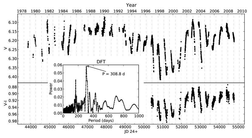
Figure 1: The photometric time series in $V$ from 1979–2009 and in $V-I$ from 1996–2009. The expected times of $V$ maxima are indicated with dashed lines. The inset shows the power spectrum from the period analysis (see Sect. 3.1).

The Wolfgang telescope was used on five dedicated nights 20–24 December 2007 to monitor the star with a cadence of 3.0 min to check for possible high-frequency photometric variations. The second night was lost due to poor weather, the third night was usable for about half of the night, the others were good. On the three nights 20th, 23rd and 24th, the target was observed for 7.5 hours continuously, on the 21st for 4.5 hours, and on the 22nd for 2 hours. The total time on target during these five nights was 29 hours of which the 2 hours on the 22nd were of poor quality and discarded. A total of 542 $y$ data points were acquired. Only Strömgren $y$ was employed. These data were calibrated to the standard Strömgren magnitudes. The external rms of the time-series is $\approx 1.2$ mmag in $y$.

2.2 Spectroscopy

We have been conducting ultra-stable radial velocity monitoring of EK Eri with HARPS (Mayor et al. 2003; Rupprecht et al. 2004) from September 2004 to April 2007, mostly with rather uneven spacing between data points. Typical exposure times were 480–600 s resulting in a typical peak S/N $\approx$ 300 for individual exposures, which translates to an intrinsic RV precision of better than 1 m s^-1 per exposure. The HARPS resolution is $R=100,000$.

Accurate radial velocities are derived by the HARPS pipeline using cross-correlation with line templates (masks). The high-precision comes from the use of a simultaneous Th-Ar calibration spectrum for accurate wavelength calibration and from the intrinsic high stability of the spectrograph. The resulting Cross-Correlation Function (CCF) is fitted with a Gaussian to obtain the RV.

In March 2007 we had three consecutive half-nights of continuous monitoring to search for oscillations and probe the asteroseismic parameters of the star. We used exposure times of 360–480 s which resulted in peak S/N $\approx$ 250–300 for individual exposures at a cadence of about 8 min. We observed for about three hours per night, obtaining a total of 70 spectra.

We have also retrieved archive data of EK Eri taken with the CES high-resolution spectrograph at ESO/La Silla Observatory. One 900 s spectrum at a central wavelength of 6155 Å was obtained on UT date 2004-09-03 and one 600 s spectrum at 6463 Å was obtained on UT date 2005-08-11. The spectra cover 39 Å and 43 Å, respectively. These data were reduced using the CES pipeline. The resolution is R $\approx 220,000$ with S/N $\approx 500$ in both spectra.

3 Results

In the following we will investigate the high-resolution spectroscopy and long-term photometric time-series data. The numerical results are summarized in Table 1.

Table 1: Summary of the properties of EK Eri.

Parameter	Value		Section
$T_{\mathrm{eff}}$	$5135$	$\pm 80$ K	3.3
$\log g$	$3.39$	$\pm 0.12$	3.3
[M/H]	$+0.02$	$\pm 0.04$	3.3
$\xi_{t}$	$1.15$	$\pm 0.03$ km s-1	3.3
$v_{\mathrm{macro}}$	$2.3$	$\pm 0.2$ km s-1	4.1
$v\sin i$ (measured)	$<1.6$	$\pm 0.4$ km s-1	4.1
$v\sin i$ (predicted)	$<0.40$ km s-1		4.1
$L/L_{\odot}$	$14.5$	$\pm 1.6$	3.4
$M/M_{\odot}$	$1.92$	$\pm 0.13$	3.4
$R/R_{\odot}$	$4.87$	$\pm 0.29$	3.4
Age	$1.1$	$\pm 0.2$ Gyr	3.4
$P_{\mathrm{rot}}$	$617.6$	$\pm 5.0$ d	4.2
$P_{\mathrm{phot}}$	$308.8$	$\pm 2.5$ d	3.1
Ephemeris	HJD$2,453,372.679+nP_{\mathrm{phot}}$		3.1

3.1 Photometric period and modulation

Strassmeier et al. (1999) determined the period of the long-term photometric variation of EK Eri based on the data obtained to that date. They also found that the period may have changed slightly when comparing the years 1978–1986 to the years 1992–1999, possibly due to distinct activity cycles. Here we derive the period using the full data set, using a variety of techniques summarized in Table 2. From these results we adopt a photometric period of $308.8\pm 2.5$ d (see inset of Fig. 1). Given the errors on the individual results and the obvious spot evolution, we cannot comfortably give the period with higher precision.

Table 2: Results from different methods of period analysis of the long-term photometry. The period has been found by a Gaussian fit to the peak, except for Period04 which uses a sinusoidal fit. The $\sigma$ is the error on the fitted peak position.

Method	Pphot [d]	$\sigma$ [d]
Period04	308.99	—
DFT	308.76	3.36
CLEAN	308.77	4.00
Lomb-Scargle	308.91	2.04
Lafler-Kinman	308.57	3.19
MSL	310.12	5.05
PDM	309.81	7.39
Adopted value	308.8	2.5

The corresponding ephemeris is given in Table 1 and is marked by dashed vertical lines in Fig. 1. As can be seen, the ephemeris can not always reproduce the data, indicating that the spots are changing size and configuration. From Fig. 1 it is clear that when the star is fainter, $V-I$ is higher (i.e., the star is redder) which points to cool spots as the cause of the variation. Since the period is likely much longer than typical spot lifetimes we cannot hope to extract any quantitative information on the amount of differential rotation.

We will now describe the methods used to derive the periods in Table 2. Both the Discrete Fourier Transform (DFT; e.g., Reegen 2007) and Period04 (Lenz & Breger 2005) were used, where we prewhitened with two long periods corresponding to long-term drifts. Period04 is developed for asteroseismic applications where the light curve can be assumed to be made up of sinusoidal components. This makes it inappropriate for our analysis of the long term variations which are changing in amplitude and possibly also in period. The usual formula for the period precision based on a mix of white and $1/f$ noise therefore has no physical meaning. The CLEAN algorithm (also known as iterative sine-wave fitting; e.g., Frandsen et al. 1995) revealed only one main peak in the resulting amplitude spectrum after pre-whitening with the long-term drifts. The Lomb-Scargle periodogram gives results similar to the DFT, but with slightly lower error. The Lafler-Kinman analysis (Lafler & Kinman 1965) gives a similar result, but the periodogram is not as convincing — a trait shared by the Minimum String Length (MSL) method. The Phase Dispersion Minimization (PDM) tend to generate higher period aliases, but even so the peak was clearly identified, although not very well determined.

3.2 Asteroseismic results

Figure 2: RV vs. BJD for the three nights of high-cadence spectra used for the asteroseismic analysis. The mean error bar is shown at the lower left corner. The three-night run displays clear variation, but with period variations from night-to-night, likely due to mode beating.

From its position in the HR diagram, EK Eri is expected to show p-mode oscillations that are stochastically excited and damped by near surface convection similar to what is observed in the Sun and other solar-like stars (Bedding & Kjeldsen 2003). We therefore carried out high-cadence ($\Delta t\approx 8\,$min) spectroscopic monitoring during three consecutive nights using HARPS as outlined in Sect. 2.2. In addition, five nights of high-cadence photometric monitoring was conducted as described in Sect. 2.1

3.2.1 Radial velocity frequency spectrum

The time series is shown in Fig. 2 and shows significant variability of a few metres per second (peak-to-peak) with periods of roughly 1 hour. The slight night-to-night offsets are likely due to slow variations in the overall activity level.

Figure 3: Fourier spectrum of the three nights of HARPS high-cadence radial velocity data. The inset shows the spectral window with the same frequency scale as the main panel.

In Fig. 3 we show the Fourier power spectrum of the time series, which shows the variability as an excess power in the frequency range 200–400$\leavevmode\nobreak\ \mu$Hz. This excess agrees with the expected frequency of maximum power estimated from scaling the solar value (Kjeldsen & Bedding 1995), which gives roughly 340 $\mu$Hz. The power at very low frequency ($\approx 50\,\mu$Hz) is predominantly caused by the slow linear trend seen on the third night and is probably not due to oscillations.

The frequency spectra of the Sun and other solar-like stars show an almost regular series of peaks. From this, one can extract the spacing between modes of successive radial order called the large separation, $\Delta\nu$, which provides a very precise measure of the mean density of the star. By scaling the solar value we find that the expected large separation of EK Eri (using the scaling formula from Kjeldsen & Bedding 1995) is around $20$ $\mu$Hz.

Due to the short and sparse coverage the present data set does not allow detection of the individual frequencies or the large separation. However, we are able to estimate the amplitude per mode from the excess power in the Fourier spectrum using the approach by Kjeldsen et al. (2005). First, the Fourier spectrum is converted into power density by dividing by the area under the spectral window. Then we convolve the spectrum with a Gaussian with a width of $4\Delta\nu$, to create just a single smooth hump of excess power and finally we multiply by $\Delta\nu/4.09$ (Kjeldsen et al. 2008) and take the square root to get the amplitude per radial mode.

Figure 4: Amplitude per radial mode. The amplitude is significantly lower than expected — compare e.g. with Fig. 8 of Kjeldsen et al. (2008). See text for explanation.

The result is shown in Fig. 4. The peak amplitude per radial mode is approximately $0.15$ m s^-1, but with a large variation from night-to-night, which is expected from the stochastic nature of the excitation mechanism. Still, this amplitude is significantly lower than expected (by at least a factor of $\approx 3$) based on results for stars with similar oscillation periods (Fig. 8 of Kjeldsen et al. 2008). Part of this discrepancy may be explained by mode beating in conjunction with the short time span of our observations. From this analysis we find the position of maximum power to be $\nu_{\rm max}=320\pm 32$ $\mu$Hz, where we have adopted a 10% uncertainty using simulated data: for this purpose we use the simulator described in Stello et al. (2004). The input mode frequencies were taken from a pulsation model of the star derived using the ADIPLS code (Christensen-Dalsgaard 2008). We calculated the individual mode amplitudes by scaling the shape of the solar excess power by the acoustic cut-off frequency and normalised to the peak amplitude found from Fig. 4. The input amplitude takes into account the different inertia of the modes and visibilities of whole-disk integrated observations. The simulations show a $\approx 10$% scatter in $\nu_{\rm max}$ and a $\approx 30$% scatter in amplitude with assumed mode lifetimes in the range 1–20 days. In addition, we tried to utilise the simulations to obtain a mode lifetime, but concluded that the data did not allow a robust estimate.

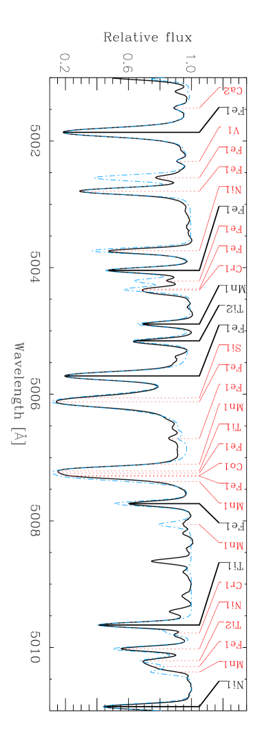
Figure 5: A section of the combined HARPS spectrum illustrating the high S/N. The observed and synthetic spectra are shown with solid and dot-dashed lines, respectively. The main lines contributing to the spectrum are marked by vertical lines. The solid vertical lines mark the least blended lines that are used in the abundance analysis.

3.2.2 Short-term photometric variations

We also searched for variability due to oscillations in the high-cadence photometric data. Of the three full nights obtained, a period analysis reveals no periodicity on two of the nights, while on a third night a single peak with a false alarm probability of 9.4% was detected at $f=26.016$ d^-1 ($301.11$ $\mu$Hz) or around 55 min at an amplitude of $\approx 5$ mmag. This frequency corresponds well to the envelope found from the spectroscopic time series. However, based on the scaling relations of Kjeldsen & Bedding (1995) and the observed RV amplitude, the photometric amplitude of EK Eri is expected to be $\approx 50$ ppm, which is a factor of 100 lower than the observed peak. Although this peak appears significant, we believe it to be an artifact.

3.3 Effective temperature, gravity, abundances

To determine the fundamental parameters of EK Eri we analysed a co-added spectrum with high S/N. This spectrum was made from the three consecutive nights of asteroseismic observations. We shifted the HARPS spectra by the individually measured velocity shifts and calculated the sum. The blue arm of the spectrum from 4402–5304 Å has S/N of 700 and the red arm from 5337–6905 Å has S/N of 1,300 in the continuum. We made a careful normalization by identifying continuum points in a synthetic spectrum with the same parameters as EK Eri. A small part of the co-added spectrum is shown in Fig. 5. Also plotted is a computed synthetic spectrum which shows some discrepancies, likely due to missing lines (e.g. 5008.7 Å) or erroneous $\log gf$ values (e.g. 5002.6 Å).

We analysed the normalized spectrum using the software package VWA (Bruntt et al. 2004, 2008). The software uses atmospheric models interpolated in the grid by Heiter et al. (2002) and atomic data from the VALD database (Kupka et al. 1999). The computation of abundances relies on synthetic spectra calculated with the SYNTH code (Valenti & Piskunov 1996).

We used VWA to automatically select 1019 of the least blended lines. However, as part of the analysis we corrected the oscillator strengths ($\log gf$) by measuring abundances for the same lines found in a spectrum of the Sun from the Atlas by Hinkle et al. (2000) (originally from Kurucz et al. 1984): 627 lines were found in common with the Sun and could be corrected, and only these lines were considered in the further analysis. This differential analysis leads to a significant improvement in the rms scatter of the abundances of Fe i and Fe ii from 0.12 to 0.06 dex. For other elements the improvement in the scatter is typically 30%.

The fundamental atmospheric parameters of EK Eri were determined by adjusting the microturbulence ($\xi_{t}$), $T_{\mathrm{eff}}$, and $\log g$ until no correlation was found between the abundances of Fe i and their equivalent width or the excitation potential and with the additional requirement that the mean Fe abundance is the same found from neutral and ionized lines. The resulting parameters are $T_{\rm eff}=5135\pm 60$ K, $\log g=3.39\pm 0.06$ and $\xi_{t}=1.15\pm 0.05$ km s^-1. We estimated the uncertainties by perturbing $\xi_{t}$, $T_{\mathrm{eff}}$  and $\log g$ in a grid around the derived values by $\pm 0.2$ km s^-1, $\pm 200$ K, and $\pm 0.2$ dex, respectively, and measuring the change in the correlations described above (see Bruntt et al. 2008). These uncertainties are “internal” errors since we assume the model atmosphere describe the actual star. We have added an addition systematic error of 50 K and 0.1 dex to $T_{\mathrm{eff}}$ and $\log g$ in Table 1.

The abundance pattern for $17$ elements is shown in Fig. 6 and listed in Table 3. The uncertainties on the abundances are the quadratic sum of the standard deviation of the mean value and the contribution due to the uncertainty on the model parameters ($\sigma_{\rm model}=0.035$ dex). Our estimate of the metallicity is based on the mean abundance of iron-peak elements with at least $10$ lines (Si, Ti, V, Cr, Fe and Ni) giving ${\rm[M/H]}=+0.02\pm 0.04$ for the combined spectrum.

From Fig. 6 we do not see evidence for peculiarities in the abundances, which might otherwise have hinted at an earlier phase as a chemically peculiar star. Any abundance peculiarities present initially in the photosphere seem to have been efficiently homogenized with the deeper layers as the star evolved off the main sequence.

Our results on the fundamental parameters and abundances are different from what we found in Paper I at a level that may seem incompatible with the uncertainties: $T_{\mathrm{eff}}$ is 100 K cooler and $\log g$ is 0.1 dex lower in our new analysis. The quality of the spectrum used in Paper I was lower and therefore only half as many lines could be used (${\rm S/N}\simeq 500$ near 6300 Å in Paper I compared to $1300$ in our new spectrum). Both analyses were done by measuring abundances differentially to the same lines in a spectrum of the Sun. In Paper I we used a sky spectrum as a proxy for the Sun, while in the current analysis we use the high-quality spectrum from Kurucz et al. (1984). This difference could introduce a systematic offset. It can be debated whether it is valid to use the differential approach since EK Eri is a more massive and evolved star compared to the Sun. In fact, the differences we find in $T_{\mathrm{eff}}$ and $\log g$ may reflect realistic uncertainties to be adopted for the star.

A more intriguing idea is that the lower $T_{\mathrm{eff}}$ we find is due to a higher amount of spot coverage at the time of observation. To investigate the evidence for changes in $T_{\mathrm{eff}}$ at different rotational epochs, we have constructed spectra by combining subsets of our new data. These four spectra, designated E1 to E4, are listed in Table 4 along with the parameters determined from them. The time intervals corresponding to these spectra are indicated in Fig. 8. Firstly, we do not see any significant abundance variation in the E1–E4 spectra. Secondly, $T_{\rm eff}$ seems to be systematically lower when the star is faint (which would be expected if it would be an effect of changes in spot coverage). However, we do not claim that the slight differences between the E1…E4 spectra are real, since the variation of $T_{\mathrm{eff}}$ and $\log g$ are only 40 K and 0.1 dex respectively, which are well within the uncertainties of the main analysis. Although the relative change in $T_{\mathrm{eff}}$ can be measured very precisely, we must consider that the model atmospheres have been interpolated from the relatively coarse grid of Heiter et al. (2002) which has a finite grid step size of 200 K in $T_{\mathrm{eff}}$ and 0.2 dex in $\log g$. This is the main argument that we do not claim the slight differences in $T_{\mathrm{eff}}$ to be a physical phenomenon.

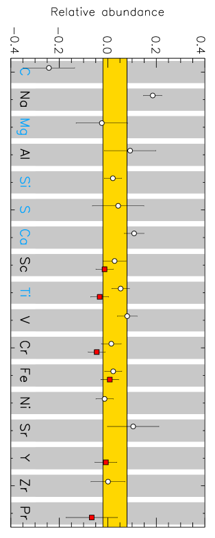
Figure 6: The abundance pattern of EK Eri measured relative to the Sun. Circles are mean abundances of neutral elements and squares are for singly ionized species.

Table 3: Abundances of 17 elements in EK Eri. The columns contain the element name and ionization stage, the mean abundance relative to the Sun, and the number of spectral lines used.

El.	$A$	$N$	El.	$A$	$N$
C i	$-0.24$	2	V i	$+0.08\pm 0.04$	15
Na i	$+0.19\pm 0.04$	3	Cr i	$+0.01\pm 0.04$	20
Mg i	$-0.02$	2	Cr ii	$-0.05\pm 0.04$	4
Al i	$+0.09$	2	Fe i	$+0.02\pm 0.04$	300
Si i	$+0.02\pm 0.04$	31	Fe ii	$+0.01\pm 0.04$	15
S i	$+0.04$	1	Ni i	$-0.01\pm 0.04$	63
Ca i	$+0.11\pm 0.04$	8	Sr i	$+0.10$	1
Sc i	$+0.03\pm 0.05$	5	Y ii	$-0.01\pm 0.04$	5
Sc ii	$-0.01\pm 0.04$	4	Zr i	$+0.00\pm 0.07$	3
Ti i	$+0.05\pm 0.04$	50	Pr ii	$-0.07$	1
Ti ii	$-0.03\pm 0.04$	11

Table 4: Results of the spectroscopic analysis using sub-sets E1–E4 of the HARPS spectra. $N$ is the number of spectra summed and S/N is for the red part of the spectrum. The photometric phase $\phi_{\mathrm{phot}}$ is relative to the ephemeris zero point given in Table 1. The phases are marked in Fig. 8. The results from the combined spectrum and from Paper I are listed for convenience.

	Time span	$\phi_{\mathrm{phot}}$	$N$	S/N	$T_{\mathrm{eff}}$ [K]	$\log g$	[Fe/H]
E1	2006-02-11 — 2006-04-02	0.31 – 0.47	5	700	$5150$	$3.34$	$+0.06$
E2	2006-07-17 — 2006-09-08	0.82 – 0.99	7	900	$5125$	$3.44$	$+0.09$
E3	2006-12-28 — 2007-01-03	0.35 – 0.37	5	530	$5165$	$3.37$	$+0.04$
E4	2007-03-29 — 2007-04-02	0.64 – 0.65	4	410	$5135$	$3.42$	$+0.06$
Comb.	2007-03-03 — 2007-03-05	0.56	70	1,300	$5135$	$3.39$	$+0.02$
Paper I	2004-10-01 — 2005-03-17		6	500	$5240$	$3.55$	$+0.09$

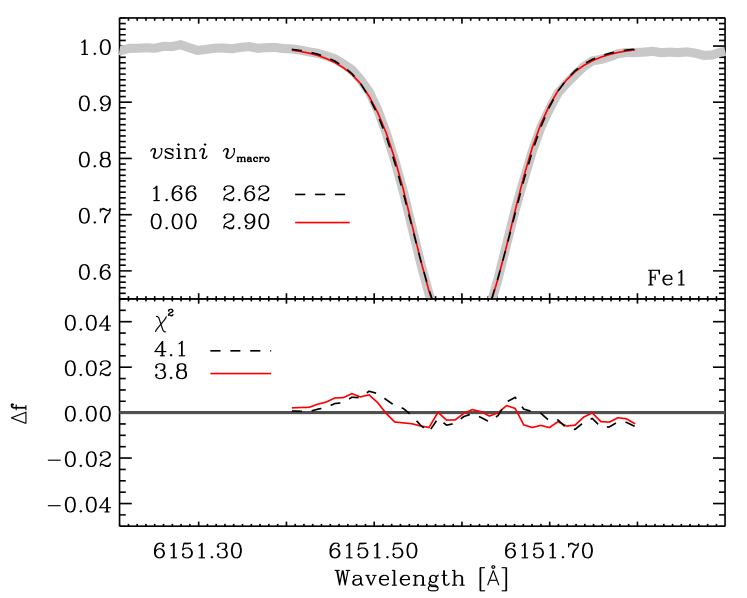
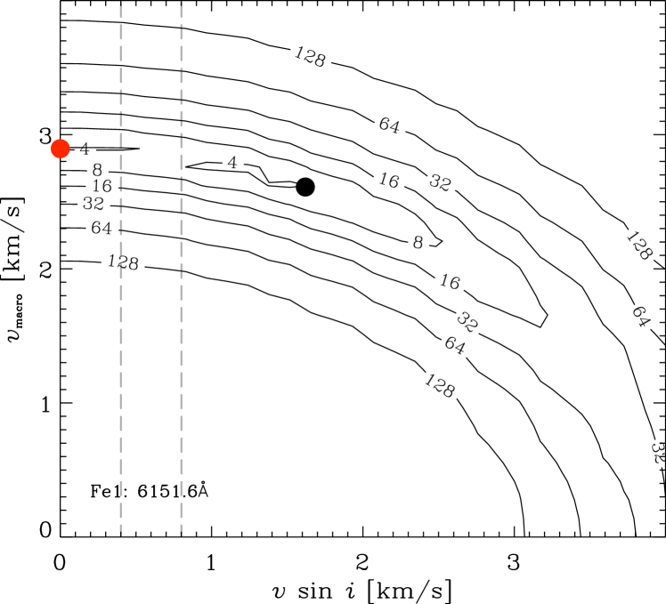
Figure 7: Synthetic profiles of the Fe i 6151.6 Å line fitted to the CES spectrum. The Upper panel shows the observed spectrum in grey, and two fits using the values of $v\sin i$ and $v_{\mathrm{macro}}$ listed. The residuals of the fits are plotted underneath. The lower panel shows the $\chi^{2}$ contours as a function of $v\sin i$ and $v_{\mathrm{macro}}$ for the same Fe line with the position of the two plotted fits marked by filled circles (red and black). Indicated with dashed vertical lines are the limits on $v\sin i$ imposed by the stellar radius and the $P_{\mathrm{rot}}=2P_{\mathrm{phot}}$ and $P_{\mathrm{rot}}=P_{\mathrm{phot}}$ alternatives.

3.4 Mass estimates

To estimate the mass of the star we followed the approach of Stello et al. (2008) by applying a scaling relation of $\nu_{\rm max}$, which includes the luminosity, effective temperature, and mass. To estimate the luminosity we use the $V$ magnitude, bolometric correction and the parallax. The magnitude $V\simeq 6.0$ is the brightest measured magnitude, hence we assume it corresponds to no or low spot activity. This value is probably only accurate to within $\pm 0.1$ mag. We adopted a bolometric correction from the tables in Bessell et al. (1998) for the $T_{\mathrm{eff}}$ and $\log g$ obtained from the spectroscopic analysis. Finally, we use the parallax $16.31\pm 0.47$ mas (van Leeuwen 2007) to get $L/L_{\odot}=14.5\pm 1.6$ and $M_{\mathrm{bol}}=1.952\pm 0.087$. To obtain the mass we use the observed value of $\nu_{\rm max}=320\pm 32$ $\mu$Hz, and get $M/M_{\odot}=2.1\pm 0.3$.

Another way to estimate the mass is to compare the location of the star in the HR diagram with theoretical isochrones or evolutionary tracks. Stello et al. (2009) compared different methods to estimate the fundamental parameters of stars from basic photometric indices. We adopted their SHOTGUN approach, which uses BASTI isochrones (Pietrinferni et al. 2004) and models without overshoot, taking as input the metallicity, effective temperature, and luminosity. The output from the program is the mass, radius and age of the star: $M/M_{\odot}=1.92\pm 0.13$, $R/R_{\odot}=4.87\pm 0.29$, and age $1.1\pm 0.2$ Gyr. From $M$ and $R$ we get $\log g=3.35\pm 0.06$, which is very similar to the value $\log g=3.39\pm 0.06$ from the spectral analysis in Sect. 3.3. Including overshoot in the BASTI models results in only slightly different values; $M/M_{\odot}=1.80\pm 0.10$, $R/R_{\odot}=4.84\pm 0.35$, age $1.5\pm 0.2$ Gyr, and $\log g=3.33\pm 0.07$. In Table 1 we list the results using the standard BASTI isochrones without overshoot.

These two independent mass estimates are in rough agreement. A seismologically determined mass estimate is potentially more accurate than isochrone fitting if one can measure the large separation $\Delta\nu$ or the position of maximum power $\nu_{\rm max}$ (Basu et al. 2009). Since our data do not allow us to measure $\Delta\nu$ and the error on $\nu_{\rm max}$ is rather large, we adopt the mass estimate based on the SHOTGUN approach.

4 Discussion

4.1 Rotation period, $v\sin i$, and radius

The rotational velocity of EK Eri is notoriously hard to measure due the the very slow rotation. The first accurate determination was done by Strassmeier et al. (1999) from $R=120,000$ spectra, from which they derived $v\sin i=1.5\pm 0.5$ km s^-1 with an adopted value of the macroturbulent velocity $v_{\mathrm{macro}}=5.0$ km s^-1, with a Fourier analysis of the line profile as a check of the validity of the adopted $v_{\mathrm{macro}}$. In Paper I we derived $v\sin i=1.0\pm 0.5$ km s^-1 by simple profile fitting to 1D atmospheric model spectra, assuming a similar value of the macroturbulence.

As we will argue in Sec. 4.2, we suggest that the rotational period of EK Eri could be twice the photometric period, i.e. close to 617 d. We have derived $4.87\pm 0.29$ R_⊙ (see Sect. 3.2), which is in good agreement with the value of $R=4.78$ R_⊙ we derive using Eq. 1 from Strassmeier et al. (1999). Adopting $P_{\mathrm{rot}}=2P_{\mathrm{phot}}$, this means that the radius of the star will be $R/R_{\odot}=12.2\,v\sin i$, where we assume that $i\simeq 90^{\circ}$. With the derived radius of $4.87$ R_⊙, this translates to an expectation for the measurement of $v\sin i$, namely $v\sin i<0.40$ km s^-1. If on the other hand $P_{\mathrm{rot}}=P_{\mathrm{phot}}$, then $v\sin i$ must be less than $0.80$ km s^-1, as already noted by Strassmeier et al. (1999), and this value can thus be regarded as a safe upper limit on $v\sin i$.

Using the high-resolution CES data, and our newly derived stellar parameters, we have attempted to derive $v\sin i$ and $v_{\mathrm{macro}}$. For this analysis we chose 7 lines from the two CES spectra, chosen to be non-blended based on the line list obtained from VALD (Kupka et al. 1999) and visual evaluation of the line symmetry. The synthetic spectrum is broadened with different values of $v\sin i$ and $v_{\mathrm{macro}}$ in a fine grid in the range 0–4 km s^-1 for both parameters, and the $\chi^{2}$ is calculated. At values of $v_{\mathrm{macro}}>4$ km s^-1 the fits start to deviate significantly and we thus note that a value of $v_{\mathrm{macro,RT}}=5$ km s^-1 (originally from Gray 1992, as a “typical” value) is inconsistent with our results.

There is a strong correlation between the broadening caused by rotation and by macroturbulence which is very difficult to separate even though their exact forms are slightly different. In general we find a continuum of solutions, as illustrated in Fig. 7, which shows the reduced $\chi^{2}$ surface for one spectral line for different values of $v\sin i$ and $v_{\mathrm{macro}}$. The $\chi^{2}$ surfaces for the other lines look very similar. We find that $v\sin i$ is so low that it cannot be determined reliably and only upper limits can be set. Note that we do not include Zeeman broadening, which in any case would contribute to an even lower limit on $v\sin i$.

4.2 Radial velocity and activity variations

It is well known that stellar magnetic activity affects the shape of spectral lines and thereby the apparent RV (Gray 1988, 2005), which again affects the ability to detect planets by the Doppler technique. The best direct measure of activity available in the HARPS spectra are the emission cores of the calcium H and K lines, and for each spectrum we have derived the activity index $R_{\mathrm{HK}}$ following the procedure of Paper I. It was shown by Queloz et al. (2001) that the Bisector Inverse Slope (BIS) of the CCF is a good qualitative measure of the distortion of the spectral lines caused by activity, and we have calculated the BIS for all CCFs following the procedure of Dall et al. (2006). The series of RV, BIS and $\log R_{\mathrm{HK}}$ are shown in Fig. 8 along with the corresponding part of the photometric light curve. In Figs. 9 and 10 we show the correlations of RV with activity index $\log R_{\mathrm{HK}}$ and BIS.

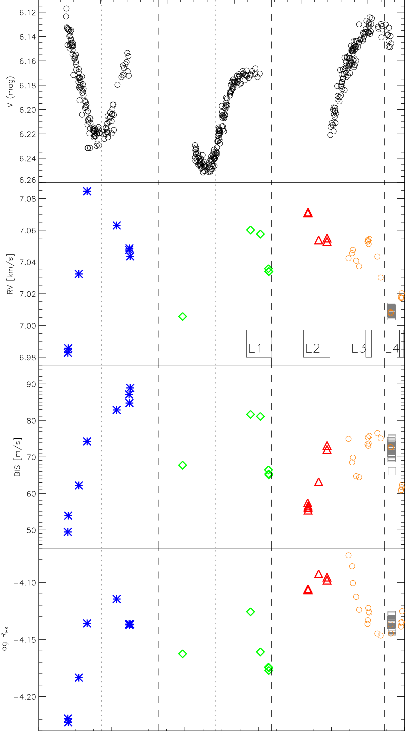
Figure 8: Comparison of the photometric and spectroscopic time series over the 3 years of simultaneous monitoring. The colors and the symbols in the 3 lower plots are: blue ($\ast$): 2004-09-30 — 2005-03-20, green ($\diamond$): 2005-08-10 — 2006-04-02, red ($\triangle$): 2006-07-17 — 2006-09-08, orange ($\circ$): 2006-11-06 — 2007-04-02 (except the three-night run in March 2007), and grey ($\Box$, at $\sim$2007.4): 2007-03-03 — 05 (3 nights of high-cadence data, cf. Fig. 2). The expected times of photometric minima (vertical dotted lines) and maxima (vertical dashed lines) are indicated. The data segments E1–E4 are marked (see Table 4 and Sect. 3.3).

Figure 9: Activity index $\log R_{\mathrm{HK}}$ vs. RV using the same symbols as in Fig. 8. The lines and arrows indicate the evolution with time. The small grey points inside the box are the 3 nights of high-cadence data. The change in activity level during these nights is only about 0.02 in $\log R_{\mathrm{HK}}$ which is much smaller than the long-term variations. The clear correlation between activity level and RV shows that the majority of the RV variations come from activity-related causes. The overall level seems to have increased between 2004-05 and 2006-07.

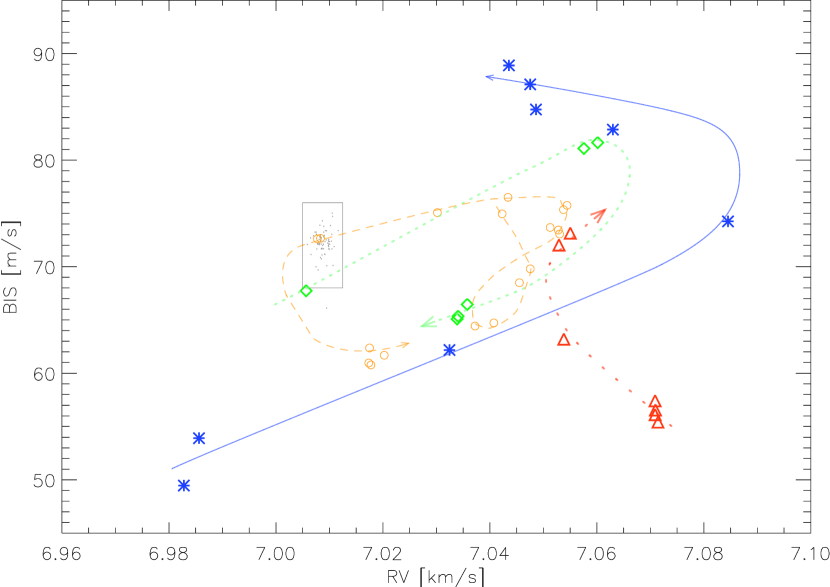
Figure 10: BIS vs. RV with the same symbols in Fig. 8 and 9. The night-to-night variation is very small and comparable with the single-night scatter. Thus, the larger scale variation in BIS, which correlates well with RV, is real and attributable to line profile variations.

From Figs. 8 and 9, it is clear that the large scale RV variations are very well correlated with the activity as measured by $\log R_{\mathrm{HK}}$. As the star gets dimmer, it gets redder (as noted by Strassmeier et al. 1999) and the chromospheric activity gets higher, both facts pointing to cool spots with overlaid plages as the cause of the variation. The variation of RV seems to be correlated with the photometric variation as well, although the correspondence is not always straightforward and the RV amplitude varies differently from the light amplitude.

The BIS shows in general a strong correlation with RV as does $\log R_{\mathrm{HK}}$. However, there seem to be significant deviations: the red points ($\triangle$ symbols), corresponding to about two months in late 2006 only, show a very distinct behavior in BIS, essentially reversing the sign of the RV-BIS correlation. This behavior is not seen in the direct activity measure $\log R_{\mathrm{HK}}$. The last observing period ($\circ$ symbols) exhibit variations in RV and $\log R_{\mathrm{HK}}$which is overall anti-correlated with the light variation, although much more complex. The BIS varies very little during this period, but like $\log R_{\mathrm{HK}}$ shows a quite complex behavior. This is in sharp contrast to the behavior of the blue points ($\ast$ symbols) where all parameters display large-amplitude, almost textbook-like behavior with $\log R_{\mathrm{HK}}$ in anti-correlation with the light variation, and the BIS and RV being phase shifted with respect to the light. Note that the internal precision on individual data points is very high as evidenced by the low scatter of the three-night run.

It is also worth noting that the obvious strong variation of bisector shape is in apparent contradiction to the finding of Saar & Donahue (1997) who found that the BIS loses its diagnostic power for extremely low $v\sin i$. Their model results were confirmed recently by Desort et al. (2007), who found that a $v\sin i$ less than the spectrograph resolution (which is certainly the case for EK Eri) should yield a constant bisector shape. This was confirmed by Bonfils et al. (2007) and Huélamo et al. (2008) who found negligible BIS-RV correlations for the slow ($v\sin i<1$ km s^-1) rotators GJ 674 and TW Hya, respectively. This is in contrast to our findings as evident from Fig. 10. Presently, we can offer no explanation of this.

Two other aspects are worth pointing out. First, while Desort et al. (2007) find the BIS-RV slope to be negative in all their simulations, we are clearly seeing mostly positive slopes, although with at least one period of negative slope as well. These authors however presented only a few models and only for main sequence stars. Secondly, while Bonfils et al. (2007) find a clear loop pattern in the plot of RV versus Ca ii H+K emission, which they interpret in terms of rotational modulation, our results are less clear, mostly due to the incomplete phase coverage. However, from the time evolution of the $\log R_{\mathrm{HK}}$–RV and BIS–RV relations as depicted in Figs. 9 and 10 we can see that there appears to be different segments of similar loop patterns for different observing seasons, which could mean that these segments of the loops are not associated with the same spot regions. Indeed, if the star is viewed equator-on, then one spot or spot group is not enough to produce a sinusoidal light curve, much less the radial velocity and activity variations.

One possible conceptual model of EK Eri is that of an oblique rotator seen close to $i=90^{\circ}$, with the magnetic axis of a dipolar field tilted with respect to the rotation axis. This assumes that we approximate the star as a single dipole, which we believe is a reasonable approximation, taking into account also the results of Aurière et al. (2008). Assuming that the magnetic poles are associated with the spots, we propose a model of EK Eri involving two large spots or spot-covered areas, located 180^∘ opposite each other. Although Aurière et al. (2008) observed no sign changes in the average longitudinal field over the photometric phase $0.21<\phi<0.83$, which would correspond to the hypothetical two spots gradually rotating into (respectively, out of) view, we note that their observations were performed during a period where EK Eri seemed to be undergoing another cycle change similar to the one of 1987–1992. During these periods the light amplitude is low, indicating that spots are small and possibly dominated by dynamo-related activity rather than by the large scale dipole field.

In this scenario, the light curve minima correspond to a spot facing the observer, which happens twice per rotation. Hence, the rotation period $P_{\mathrm{rot}}$ of the star is not equal to $P_{\mathrm{phot}}$, but rather twice that. This would mean that the true latitude-averaged rotation period of EK Eri is $P_{\mathrm{rot}}=617.6$ d. The possibility of $P_{\mathrm{rot}}$ being two or even three times the photometric period was also mentioned by Aurière et al. (2008) but not investigated further. Such a relationship has been observed for the Sun (e.g., Durrant & Schroeter 1983) where the rotation of active regions across the solar disk gives rise to a 13-day period, i.e., half the solar rotation period. The phenomenon of $P_{\mathrm{rot}}=2P_{\mathrm{obs}}$ has also been suggested for Procyon (Arentoft et al. 2008). Note that the period $2P_{\mathrm{obs}}$ would not show up in the period analysis unless the spots were of uneven size and stable over several rotations, which is clearly not the case.

Although simple, this would explain the differences seen in the $\log R_{\mathrm{HK}}$–RV loop patterns which seem to change direction for every second loop, while also qualitatively explaining the appearance of the light curve. Of course, we are assuming that the field is poloidal, that the spots are associated with the large scale field, and that the star is seen equator-on. We have however not been able to produce a spot model that could reproduce the light curve satisfactorily using this simple geometry, and the true structure of the magnetic field and the activity of EK Eri is likely far more complex.

4.3 Photometric period changes

As evident from the light curve (Fig. 1) and as noted by Strassmeier et al. (1999), the photometric period of EK Eri is not stable. In fact, based on the latest data, the star appears to be going through a phase similar to the period 1987–1992 where the light variations almost disappeared and the period changed significantly. While this may be explained by distinct magnetic cycles, other explanations have been proposed in view of the unusually long period. One possibility proposed hypothetically by Strassmeier et al. (1990) was that the star is seen pole-on and that the long period reflects activity cycles on a rapidly rotating star. Alternatively, they suggested a strong internal rotation gradient to explain the activity in terms of a classical $\alpha\Omega$ dynamo. Stȩpień (1993) proposed the elegant solution that EK Eri is the descendant of a magnetic Ap star. Up to 10% of Ap stars have rotation periods longer than 100 d (e.g., Mathys 2008), and a significant fraction of the field should be able to survive main sequence evolution (Moss 2003).

4.4 Magnetic field geometry, and low-amplitude stellar oscillations

Aurière et al. (2008) observed modulations of the magnetic field strength with rotational phase, but they were unable to relate it to the photometric period. In particular, they observed a peak in the field strength at one phase, which they assign as their phase zero point. From our ephemeris given in Table 1 we find that their zero phase corresponds to $\phi_{\mathrm{phot}}=0.21$ in our data i.e., very close to quarter photometric phase.

In our RV monitoring, we have covered the interval from time of photometric minimum ($\phi_{\mathrm{phot}}=0$) to first quarter phase on two segments of the light curve; in 2004–5 and 2006–7 (see Fig. 8). In the first segment, all parameters vary smoothly. As we noted, this is the classical textbook behavior. In the second segment, the activity level as inferred by $\log R_{\mathrm{HK}}$ is overall higher, with the maximum level likely to have been reached just before 2006-11-06, but after the time of light minimum, i.e. around $\phi_{\mathrm{phot}}=0.1$–$0.2$. It is likely then, that the high field strength measured by Aurière et al. (2008) corresponds to a similar high value of $\log R_{\mathrm{HK}}$ and vice versa. Furthermore, around $\phi_{\mathrm{phot}}=0.2$ in 2006–7, the BIS changes direction for a short while, which may indicate an additional contribution on top of the main spot (group), possibly a smaller bright spot, or the emergence of a short lived spot. If an $\alpha^{2}$ dynamo can work locally to augment a large scale seed field at small scales on the stellar disk (a mechanism proposed for AGB stars by Soker & Zoabi 2002), then this spike could be caused by spots with completely different characteristics in terms of size and temperature, appearing alongside the semi-static fossil field-induced spots responsible for the main light modulation.

The magnetic field geometry suggested by Aurière et al. (2008) is close to a dipole, which makes intuitive sense for a remnant static field. One may expect a large scale magnetic field to have a stabilizing effect on the overall shape of the star, i.e., resisting deformations caused by the oscillations. As noted by Braithwaite (2009), a dominantly poloidal field tends to align the magnetic axis perpendicular to the rotation axis, thereby contributing to making the star oblate, even for very slow rotation. With this in mind, the surprisingly low oscillation amplitude-per-radial-mode (cf. Sect. 3.2.1) may have a logical explanation. In most stars, the $l=1$ modes are expected to have the highest amplitudes, but if the low-degree modes are suppressed, then the bulk of the oscillations will be higher degree modes. Assuming an expected amplitude per mode of $\approx 0.5$ m s^-1 (Fig. 8 of Kjeldsen et al. 2008) we find a spatial response scaling factor $S_{l}/S_{0}=0.3$. Comparing with Table 1 of Kjeldsen et al. (2008) we then propose that the bulk of the oscillations in EK Eri could be higher degree modes of $l=3,4$. Coincidentially, for the rapidly oscillating magnetic Ap stars (roAp), which are possible progenitors of EK Eri, there is emerging evidence for interaction between the magnetic field and the oscillation driving mechanism (e.g., Saio et al. 2009, and references therein).

Of course our time coverage is very poor and the discrepancy may very well be due to mode beating and the stochastic nature of mode excitation. Obviously, longer observing runs are required to test this scenario. It is interesting to note that the magnetic field measurement of Aurière et al. (2008) as well as our asteroseismic results were obtained while the star was apparently entering another “bright” phase akin to the 1987–1992 period. In order to test the interaction between the magnetic field and the oscillations it would be highly desirable to conduct asteroseismic measurements in periods of high field strength as well as in periods of relatively low field strength.

5 Conclusions

We have presented results from an intensive monitoring of the active sub-giant star EK Eri. We have used photometric data covering 30 years and spectroscopic data probing long-term variation in activity during 3 years and high-cadence radial-velocity monitoring from 3 nights. From the photometry we have refined the rotation period and the ephemeris as listed in Table 1. Also, from 3 half-nights of high-cadence RV monitoring we have detected solar-like oscillations in a late-type spotted sub-giant star for the first time. While oscillations have been detected in a number of late-type giants (e.g., Hekker et al. 2009; Hatzes & Zechmeister 2008) and for mildly active solar-type stars (e.g., Pollux: Hatzes & Zechmeister 2007; Aurière et al. 2009), this is the first detection for a sub-giant hosting a strong magnetic field. Unfortunately our data do not allow us to resolve individual frequencies. We measure an amplitude per radial mode of $\approx 0.15$ m s^-1 at a position of maximum power $\nu_{\mathrm{max}}=320\pm 32$ $\mu$Hz. This amplitude is at least a factor of 3 lower than expected and, if confirmed, may mean that the magnetic field has a strong stabilizing effect on the stellar geometry, essentially favoring high-degree oscillation modes in the presence of a near-dipole magnetic field. In that case, the interpretation of the asteroseismic data may become more difficult for this and other sub-giant stars with similar magnetic properties. A longer time series is required in order to obtain quantitative results. For reference purposes, having accurate oscillation data for a non-active star at the position in the HR diagram of EK Eri would be highly desirable. Unfortunately, neither CoRoT nor Kepler apparently covers this.

Based on the roughly sinusoidal shape of the light curve, the likely very high inclination, the field geometry suggested by Aurière et al. (2008), and the behavior of the activity indicators as function of RV, we suggest a conceptual model of EK Eri with two large low-latitude spot covered areas approximately $180^{\circ}$ apart on a star viewed equator-on. In this scenario, the rotational period is twice the photometric period, thus $P_{\mathrm{rot}}=2P_{\mathrm{phot}}=617.6$ d. We note however, that a simple two-spot model is not able to account for all the seasonal light variations observed, mostly due to the unknown spot lifetimes, sizes and longitudes.

Regardless of the rotation period, the measured values of $v\sin i$ both from this work and from the literature are inconsistent with the derived radius of the star. Both the radius derived from asteroseismology and from the spectral analysis set strict upper limits on $v\sin i$ which are lower than previous estimates. We thus conclude that the $v\sin i$ is too low to be reliably measured with available spectrographs.

Based on high-quality HARPS spectra we have derived the atmospheric parameters of EK Eri to very high precision. The abundance pattern for 17 analysed elements is very similar to the Sun, and we detect no anomalies that could otherwise be attributed to an earlier evolutionary state as a magnetic Ap star. However, in order to argue for or against EK Eri being a descendant of a magnetic Ap star, stronger constraints on the mass and evolutionary state are needed. Further seismic studies, preferably at varying rotational phases, may deliver such constraints in terms of accurate asteroseismic mass and radius measurements, and are also needed to probe the possible link between solar-like oscillations and the magnetic field.