Free Energy Methods for Bayesian Inference: Efficient Exploration of Univariate Gaussian Mixture Posteriors

Abstract

Because of their multimodality, mixture posterior distributions are difficult to sample with standard Markov chain Monte Carlo (MCMC) methods. We propose a strategy to enhance the sampling of MCMC in this context, using a biasing procedure which originates from computational Statistical Physics. The principle is first to choose a “reaction coordinate”, that is, a “direction” in which the target distribution is multimodal. In a second step, the marginal log-density of the reaction coordinate with respect to the posterior distribution is estimated; minus this quantity is called “free energy” in the computational Statistical Physics literature. To this end, we use adaptive biasing Markov chain algorithms which adapt their targeted invariant distribution on the fly, in order to overcome sampling barriers along the chosen reaction coordinate. Finally, we perform an importance sampling step in order to remove the bias and recover the true posterior. The efficiency factor of the importance sampling step can easily be estimated a priori once the bias is known, and appears to be rather large for the test cases we considered.

A crucial point is the choice of the reaction coordinate. One standard choice (used for example in the classical Wang-Landau algorithm) is minus the log-posterior density. We discuss other choices. We show in particular that the hyper-parameter that determines the order of magnitude of the variance of each component is both a convenient and an efficient reaction coordinate.

We also show how to adapt the method to compute the evidence (marginal likelihood) of a mixture model. We illustrate our approach by analyzing two real data sets.

Keywords: Adaptive Biasing Force; Adaptive Biasing Potential; Adaptive Markov chain Monte Carlo; Importance sampling; Mixture models.

1 Introduction

Mixture modeling is presumably the most popular and the most flexible way to model heterogeneous data; see e.g. Titterington et al. (1986), McLachlan and Peel (2000) and Frühwirth-Schnatter (2006) for an overview of applications of mixture models. Due to the emergence of Markov chain Monte Carlo (MCMC), interest in the Bayesian analysis of such models has sharply increased in recent years, starting with Diebolt and Robert (1994). However, MCMC analysis of mixtures poses several problems (Celeux et al., 2000; Jasra et al., 2005). In this paper, we focus on the difficulties arising from the multimodality of the posterior distribution.

For the sake of exposition, we concentrate our discussion on univariate Gaussian mixtures, but we explain in the conclusion (Section 6) how our ideas may be extended to other mixture models. The data vector $y=(y_{1},\ldots,y_{n})$ contains independent and identically distributed (i.i.d.) real random variables with density

$$p(y|\theta)=\prod_{i=1}^{n}p(y_{i}|\theta),\qquad p(y_{i}|\theta)=\sum_{k=1}^{K}q_{k}\,\varphi(y_{i};\mu_{k},\lambda_{k}^{-1}),$$ (1)

where the vector $\theta$ contains all the unknown parameters, i.e. the mixture weights $q_{1},...,q_{K-1}$, the means $\mu_{1},\ldots,\mu_{K},$ the precisions $\lambda_{1},\ldots,\lambda_{K}$, and possibly hyper-parameters, and $\varphi(\cdot;\mu,\lambda^{-1})$ denotes the Gaussian density with mean $\mu$ and variance $\lambda^{-1}$.

This model is not identifiable, because both the likelihood and the posterior density are invariant by permutation of components, provided the prior is symmetric. This is the root of the aforementioned problems. By construction, any local mode of the posterior density admits $K!-1$ symmetric replicates, while a typical MCMC sampler recovers only one of these $K!$ copies. A possible remedy is to introduce steps that permute randomly the components (Frühwirth-Schnatter, 2001). However, mixture posterior distributions are often “genuinely multimodal”, following the terminology of Jasra et al. (2005): The number of sets of $K!$ equivalent modes is often larger than one; see also Marin and Robert (2007, Chap. 6) for an example of a multimodal posterior distribution generated by an identifiable mixture model, and Section 2.2 of this paper for an example based on real data. Therefore, and following Celeux et al. (2000) and Jasra et al. (2005), we consider that a minimum requirement of convergence for a MCMC sampler is to visit all possible labelling of the parameter, without resorting to random permutations.

Inspired by techniques used in molecular dynamics (Lelièvre et al., 2010), our aim is to develop samplers that meet this requirement, using an importance sampling strategy where the importance sampling function is the marginal distribution of a well chosen variable. The principle of the method is (i) to choose a “reaction coordinate”, namely a low-dimensional function of the parameters $\theta$; (ii) to compute the marginal log-density of this reaction coordinate (minus this log-density is called the “free energy” in the molecular dynamics literature); and (iii) to use the free energy to build a bias for the target of the MCMC sampler, in order to move more freely between the different modal regions of the initial target distribution. More precisely, the biased log-density is obtained by adding the free energy to the target log-density; this changes the marginal distribution of the reaction coordinate into a uniform distribution (within chosen bounds). At the final stage of the algorithm, the bias can be removed by performing a simple importance sampling step from the biased posterior distribution to the original unbiased posterior distribution. Expectations with respect to the posterior distribution may be computed from the weighted sample. We also derive a method for computing the evidence (marginal likelihood).

If the reaction coordinate is well chosen, it is likely that a MCMC sampler targeted at the biased posterior converges to equilibrium much faster than a standard MCMC sampler, see Lelièvre et al. (2008). Two questions are then in order: How to choose the reaction coordinate? And how to compute the free energy?

Concerning the choice of the reaction coordinate, the application of free energy based methods to mixture models is not straightforward. In many cases, samplers targeting a mixture posterior distribution are metastable: This term means that the trajectory generated by the algorithm remains stuck in the vicinity of some local attraction point for very long times, before moving to a different region of the accessible space where it again remains stuck. We show that the degree of metastability of a sampler targeting a mixture posterior distribution is strongly determined by certain hyper-parameters, typically those that calibrate in the prior the spread of each Gaussian component. We show that such hyper-parameters are good reaction coordinates, in the sense that (i) it is possible to efficiently compute the associated free energy (by adaptive algorithms, see below), (ii) the corresponding free energy biased dynamics explores quickly the (biased) posterior distribution, and (iii) the points sampled from the biased distribution have non-negligible importance weights with respect to the original target posterior distribution. Other reaction coordinates are discussed, such as the posterior log-density, which is also a good reaction coordinate (with the problem however that an appropriate range of variation for this reaction coordinate, which is needed for the method, is difficult to determine a priori). This reaction coordinate is the standard choice for the Wang-Landau algorithm, see for instance Atchadé and Liu (2010), Liang (2005) and Liang (2010) for related works in Statistics.

To compute the free energy, we resort to adaptive biasing algorithms (Darve and Pohorille, 2001; Hénin and Chipot, 2004; Marsili et al., 2006; Lelièvre et al., 2007). In contrast with the adaptive MCMC algorithms usually considered in the statistical literature (see the review of Andrieu and Thoms (2008) and references therein), these adaptive algorithms modify sequentially the targeted invariant distribution of the Markov chain, instead of the parameters of the Markov kernel. Such algorithms were initially designed to compute the free energy in molecular dynamics; see also Lelièvre et al. (2010) for a recent review of alternative standard techniques in molecular dynamics for computing the free energy, such as e.g. thermodynamic integration.

It is of course possible to combine our approach with other strategies aimed at overcoming multimodality, such as tempering methods; see e.g. Iba (2001); Neal (2001) and Celeux et al. (2000).

The paper is organized as follows. Section 2 presents the univariate Gaussian mixture model, and the difficulties encountered with classical MCMC algorithms. Section 3 describes the method we propose, which is based on free energy biased dynamics. Section 4 explains how to apply this method to Bayesian inference on Gaussian mixture models. Section 5 illustrates our approach with two real data-sets. Section 6 discusses further research directions, in particular how our approach may be extended to other Bayesian models.

2 Scientific context

2.1 Gaussian mixture posterior distribution

As explained in the introduction, we focus on the univariate Gaussian mixture model (1), associated with the following prior, taken from Richardson and Green (1997), which is symmetric with respect to the components $k=1,\ldots,K$:

$$\mu_{k} \sim \mathrm{N}(m,\kappa^{-1}),$$

$$\lambda_{k} \sim \mathrm{Gamma}(\alpha,\beta),$$

$$\beta \sim \mathrm{Gamma}(g,h),$$

$$(q_{1},\ldots,q_{K-1}) \sim \mathrm{Dirichlet}_{K}(1,\ldots,1).$$

In our examples, we take $m=M$, $\kappa=4/R^{2}$, $\alpha=2$, $g=0.2$, $h=100g/\alpha R^{2}$, where $R$ and $M$ are respectively the range and the mean of the observed data, as in Jasra et al. (2005). The posterior density reads

$$p(\theta|y) = \frac{1}{Z_{K}}p(\theta)p(y|\theta)$$

$$= \frac{\kappa^{K/2}g^{h}\beta^{K\alpha+g-1}}{Z_{K}\Gamma(\alpha)^{K}\Gamma(g)(2\pi)^{\frac{n+K}{2}}}\left(\prod_{k=1}^{K}\lambda_{k}\right)^{\alpha-1}\exp\left\{-\frac{\kappa}{2}\sum_{k=1}^{K}(\mu_{k}-M)^{2}-\beta\left(h+\sum_{k=1}^{K}\lambda_{k}\right)\right\}$$

$$\times\prod_{i=1}^{n}\left[\sum_{k=1}^{K}q_{k}\lambda_{k}^{1/2}\exp\left\{-\frac{\lambda_{k}}{2}(y_{i}-\mu_{k})^{2}\right\}\right].$$

In this expression, $\theta$ is the vector

$$\theta=(q_{1},\ldots,q_{K-1},\mu_{1},\ldots,\mu_{K},\lambda_{1},\ldots,\lambda_{K},\beta)\in\Omega=\mathcal{S}_{K}\times{\mathbb{R}}^{K}\times({\mathbb{R}}_{+})^{K+1},$$ (3)

the set

$$\mathcal{S}_{K}=\left\{(q_{1},\ldots,q_{K-1})\in({\mathbb{R}}_{+})^{K-1},\ \ \sum_{i=0}^{K-1}q_{i}\leq 1\right\}$$

is the probability simplex, and

$$Z_{K}=\int_{\Omega}p(\theta)p(y|\theta)\,d\theta$$ (4)

is the normalizing constant (namely the marginal likelihood in $y$), which depends on $K$ and $y$.

The sampling of the posterior distribution with density (2.1) is the focus of the paper.

2.2 Metastability in Statistical Physics

In this section, we draw a parallel between the problem of sampling (2.1) and the problem of sampling Boltzmann-Gibbs probability measures that arise in computational Statistical Physics; see for instance (Balian, 2007). We take this opportunity to introduce some of the concepts and terms of computational Statistical Physics that are relevant in our context.

In computational Statistical Physics, one is often interested in computing average thermodynamic properties of the system under consideration. This requires sampling a Boltzmann-Gibbs (probability) measure

$$\pi(\theta)=\frac{1}{Z}\exp\left\{-V(\theta)\right\},\qquad Z=\int_{\Omega}\exp\left\{-V(\theta)\right\}\,d\theta,$$ (5)

where $\theta\in\Omega\subset{\mathbb{R}}^{d}$, and $V$ is the potential of the system, assumed to be such that $Z<\infty$. From now on, the term potential refers to the logarithm of a given (possibly unnormalized) probability density: e.g. $V(\theta)=-\log\{p(\theta)p(y|\theta)\}$ for the posterior density (2.1).

Probability densities such as the posterior density (2.1) for mixture models, or the Boltzmann-Gibbs density (5) for systems in Statistical Physics, are often multimodal. Standard sampling strategies, for instance the Hastings-Metropolis algorithm (Metropolis et al., 1953; Hastings, 1970) generate samples which typically remain stuck in a small region around a local maximum (also called local mode) of the sampled distribution (or, equivalently, a local minimum of the potential $V$). The sequences of samples generated by these algorithms are said to be metastable.

Figure 1 illustrates this phenomenon, in the Bayesian mixture context, for the posterior (2.1), with $K=3$ components, and for two datasets (Fishery data, see Section 5.1, and Hidalgo stamps data, see Section 5.2). The posterior density admits at least $K!=6$ equivalent modes, but very few mode switchings (if any) are observed in the MCMC trajectories. A simple Gaussian random walk Hastings-Metropolis is used, but we obtained the same type of plots (not shown) with Gibbs sampling.

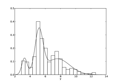
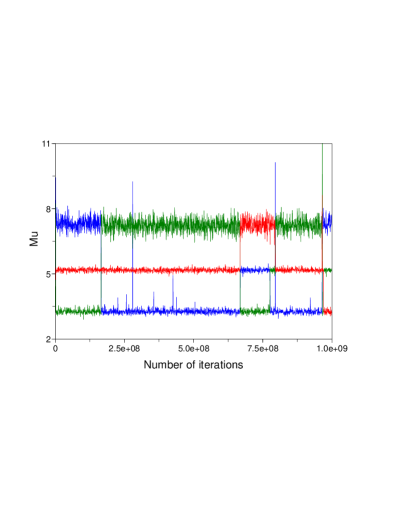
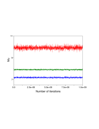
Figure 1: Left (resp. right) hand side corresponds to Fishery (resp. Hidalgo stamps) dataset. Top row: histograms of the data and an estimated 3-component Gaussian mixture probability density function (solid line). The dashed line corresponds to a local mode of the posterior density. Bottom row: random walk Hastings-Metropolis trajectories of $(\mu_{1},\mu_{2},\mu_{3})$ as a function of the number of iterations. See Section 5 for more details on the data and the sampler.

The top right plot of Figure 1 also represents a Gaussian mixture probability density (in dashed line) which corresponds to a negligible (in terms of posterior probability) local mode of the posterior density for the Hidalgo dataset. In numerical tests not reported here, when this local mode is used as a starting point, the Hastings-Metropolis sampler used needs about $T=10^{5}$ iterations to leave the attraction of this meaningless mode. It is easy to make this problem worse by slightly changing the data. For instance, $T$ is increased to $10^{7}$ by adding 2 to the three largest $y_{i}$’s (while this local mode remained of very small posterior probability). This local mode illustrates the typical “genuine multimodality” of mixture posteriors mentioned in the introduction – multimodality which cannot be cured by label permutation.

3 Free-energy biased sampling

Consider a generic probability density $\pi(\theta)$, with $\theta\in\Omega\subset{\mathbb{R}}^{d}$ as defined in (5). The principle of free energy biased sampling (described more precisely in Section 3.1) is to change the original density $\pi$ to the biased density:

$$\pi_{A}(\theta)\propto\pi(\theta)\exp\left\{(A\circ\xi)(\theta)\right\},$$

where $\xi$ is some real-valued function

$$\xi\,:\Omega\to[z_{\rm min},z_{\rm max}]$$

where $[z_{\rm min},z_{\rm max}]\subset\mathbb{R}$ is a bounded interval, $(A\circ\xi)(\theta)=A(\xi(\theta))$, and the so-called free energy $A$ (see definition (6) below) is such that the distribution of $\xi(\theta)$ when $\theta$ is distributed according to $\pi_{A}$ is uniform over the interval $[z_{\min},z_{\max}]$. By sampling $\pi_{A}(\theta)\,d\theta$ rather than $\pi(\theta)\,d\theta$, the aim is to remove the metastability in the direction of $\xi$. Averages with respect to the original distribution of interest $\pi(\theta)\,d\theta$ are finally obtained by standard importance sampling (see Section 3.3). We assume first that $\xi(\theta)$ takes values in a bounded interval $[z_{\rm min},z_{\rm max}]$, (think of $\xi(\theta)=q_{1}$ and $[z_{\rm min},z_{\rm max}]=[0,1]$ for the mixture posterior distribution case), and postpone the discussion of how to treat reaction coordinates with values in an unbounded domain to Section 3.4.

An important part of the algorithm is to compute (an approximation of) the free energy $A$. There are many ways to this end. We describe a class of methods which are very efficient in the field of computational Statistical Physics (see Section 3.2) and which, to our knowledge, have not been used so far in Statistics.

3.1 Principle of the method

Consider the conditional probability measures associated with $\xi$:

$$\pi^{\xi}(d\theta\mid\xi(\theta)=z)=\frac{\displaystyle\exp\{-V(\theta)\}\,\delta_{\xi(\theta)-z}(d\theta)}{\displaystyle\int_{\Sigma(z)}\exp\{-V(\theta^{\prime})\}\,\delta_{\xi(\theta^{\prime})-z}(d\theta^{\prime})},$$

where $\delta_{\xi(\theta)-z}(d\theta)$ is a measure with support

$$\Sigma(z)=\Big{\{}\theta\in\Omega\ \Big{|}\ \xi(\theta)=z\Big{\}},$$

defined by the formula: for all smooth test functions $\varphi$ and $\psi$,

$$\int_{\Omega}\psi(\xi(\theta))\varphi(\theta)\,d\theta=\int\psi(z)\int_{\Sigma(z)}\varphi(\theta)\,\delta_{\xi(\theta)-z}(d\theta)\,dz.$$

The main assumption underlying free-energy biased methods is that the function $\xi$ is chosen so that the sampling of $\pi^{\xi}(d\theta\mid\xi(\theta)=z)$ is significantly “easier” than the sampling of $\pi(\theta)\,d\theta$, at least for some values of $z$. In other words, $\pi^{\xi}(d\theta\mid\xi(\theta)=z)$ should be much less multimodal than $\pi(\theta)\,d\theta$, at least for some values of $z$, see the discussion in Section 4.2 below.

To give a concrete example, consider the choice $\xi(\theta)=q_{1}$. In this case, $\pi^{\xi}(d\theta\mid\xi(\theta)=z)$ is the conditional posterior distribution of all variables except $q_{1}$, conditionally on $q_{1}=z$.

The function $\xi$ is called a reaction coordinate in the physics literature, because of its physical interpretation: this function $\xi$ parameterizes the progress of some chemical event at a coarser scale (chemical reaction or change of conformation for example). Given the trajectory $\{\theta_{t}\}_{t\geq 0}$ of a Markov chain, $\xi(\theta_{t})$ is typically a metastable trajectory, and varies on timescales much larger than the typical microscopic fluctuations of the system around its metastable configurations. Of course, in our Bayesian mixture context, this physical interpretation is not very useful. For the moment, we stick with the more generic (and informal) understanding mentioned at the beginning of this paragraph, i.e. the sampling of $\pi^{\xi}(d\theta\mid\xi(\theta)=z)$ should be “easier” than the sampling of $\pi(\theta)\,d\theta$. We defer the important discussion on how to interpret and choose this “reaction coordinate” in our specific context to Section 4.2. We also refer the readers to Lelièvre et al. (2008); Lelièvre and Minoukadeh (2011) for a precise quantification of this concept in a functional analysis framework. Finally, although we consider only one-dimensional reaction coordinates in this paper, we mention that extensions to reaction coordinates with values in $\mathbb{R}^{m}$ with $m\geq 2$ are possible (Lelièvre et al., 2010; Chipot and Lelièvre, 2010). Some algorithms allowing to switch between different reaction coordinates have also been developed (Piana and Laio, 2007).

The free energy $A(z)$ is defined as

$$\exp\left\{-A(z)\right\}=\int_{\Sigma(z)}\exp\left\{-V(\theta)\right\}\,\delta_{\xi(\theta)-z}(d\theta),$$ (6)

see for instance Section 5.6 in Balian (2007). In other words, the free energy is minus the marginal log-density of the reaction coordinate. As above, let us again consider the simple example when the reaction coordinate is $\xi(\theta)=q_{1}$. Then, the free-energy is simply, up to an additive constant, equal to

$$A(q_{1})=-\log\left(\int_{\mathcal{S}_{K-1}(q_{1})\times{\mathbb{R}}^{K}\times({\mathbb{R}}_{+})^{K+1}}\exp\left\{-V(\theta)\right\}\,dq_{2}\ldots dq_{K-1}\,d\mu_{1}\dots d\mu_{K}\,d\lambda_{1}\dots d\lambda_{K}\,d\beta\right),$$

where

$$\mathcal{S}_{K-1}(q_{1})=\left\{(q_{2},\dots,q_{K-1})\in({\mathbb{R}}_{+})^{K-2},\ \ \sum_{i=2}^{K-1}q_{i}=1-q_{1}\right\}.$$

In words, the free energy is in this case the opposite of the log-marginal density of $q_{1}$.

The free energy can be used to bias the target density $\pi$ as follows:

$$\pi_{A}(\theta)=\frac{1}{Z_{A}}\exp\left\{-V(\theta)+(A\circ\xi)(\theta)\right\}.$$

We refer to densities of this form as free energy-biased densities. The essential property of $\pi_{A}(\theta)$ is that, by construction, the corresponding marginal distribution of $\xi$ is uniform on the interval $[z_{\min},z_{\max}]$. A sampler targeting $\pi_{A}(\theta)\,d\theta$ is thus much less likely to be metastable (namely to get stuck around a local minimum of the density) than a sampler targeting $\pi(\theta)\,d\theta$, because (i) the former sampler should move freely along the direction $\xi(\theta)$ defined by the reaction coordinate, since the marginal distribution of $\xi(\theta)$ is uniform, and (ii) we have assumed that the reaction coordinate $\xi(\theta)$ is such the conditional probability distributions $\pi_{A}^{\xi}(d\theta\mid\xi(\theta)=z)=\pi^{\xi}(d\theta\mid\xi(\theta)=z)$ are easy to sample, at least for some values of $z$ (namely that they do not have very separated modes).

Therefore, free energy-based methods aim at sampling $\pi_{A}(\theta)$, in order to move freely across the sampling space. Then, $\pi$ is eventually recovered through an importance sampling step, from $\pi_{A}$ to $\pi$: for any test function $\varphi$,

$$\mathbb{E}^{\pi}(\varphi)=\int_{\Omega}\varphi(\theta)\,\pi(\theta)\,d\theta=\frac{\displaystyle\int_{\Omega}\varphi(\theta)\exp\left\{-A\circ\xi(\theta)\right\}\,\pi_{A}(\theta)\,d\theta}{\displaystyle\int_{\Omega}\exp\left\{-A\circ\xi(\theta)\right\}\,\pi_{A}(\theta)\,d\theta}=\frac{\displaystyle\mathbb{E}^{\pi_{A}}\Big{(}\varphi\exp\left\{-A\circ\xi\right\}\Big{)}}{\displaystyle\mathbb{E}^{\pi_{A}}\Big{(}\exp\left\{-A\circ\xi\right\}\Big{)}}.$$ (7)

We refer to Section 3.3 for further precisions. Note that for (7) to hold, $A$ only needs to be defined up to an additive constant.

3.2 Computing the free energy by adaptive methods

In most cases, the free energy $A$ defined in (6) does not admit a closed-form expression, and must be estimated. There are nowadays many techniques to this end, with various degrees of efficiencies and conceptual complexities. We present in this section some powerful algorithms, namely adaptive biasing methods, which are not so well known in the statistical literature. Of course, any other standard method such as thermodynamic integration could be used (see the book (Lelièvre et al., 2010) for a precise presentation of standard methods for free energy computations in the framework of computational Statistical Physics, as well as Gelman and Meng (1998) for a review from the viewpoint of Statistics).

3.2.1 General structure of adaptive methods

In adaptive biasing Markov chain Monte Carlo methods, a time-varying biasing potential $A_{t}(z)$ is considered. The biasing potential $A_{t}$ is sequentially updated in order to converge to the free energy $A$ in the limit. As already mentioned in the introduction, the term “adaptive” refers in this paper to the dynamic adaptation of the targeted probability measure, and not of the parameters of a Markov kernel used in the simulations. Specifically, at iteration $t$, the time-varying targeted density is

$$\pi_{A_{t}}(\theta)=\frac{1}{Z_{A_{t}}}\exp\left\{-V(\theta)+(A_{t}\circ\xi)(\theta)\right\}.$$ (8)

An adaptive MCMC algorithm simulates a non-homogeneous Markov chain $(\theta_{t})$, $t=1,2,\ldots$, using the two following steps at iteration $t$:

1. a MCMC move according to the current target $\pi_{A_{t}}$ defined in (8),

   $$\theta_{t}\sim K_{t}(\theta_{t-1},\cdot),$$

   where $K_{t}$ is a Markov kernel leaving $\pi_{A_{t}}$ invariant;

2. the update of the bias to $A_{t+1}$, using a trajectory average, see Section 3.2.2 below.

The first step may be done using a Hastings-Metropolis kernel for instance, see Figure 2.

Before explaining the second step, let us mention how the discretization of the reaction coordinate values for the biasing potential $A_{t}$ is done in practice. A simple strategy, which we adopt in this paper, is to use predefined bins, and approximate the biasing potential $A_{t}$ or its derivative $A_{t}^{\prime}$ (with respect to $z$) by piecewise constant functions. Specifically, we consider $N_{z}$ bins of equal sizes $\Delta z$,

$$[z_{\rm min},z_{\rm max}]=\bigcup_{i=0}^{N_{z}-1}[z_{i},z_{i+1}],\quad z_{i}=z_{\rm min}+i\Delta z,\quad\Delta z=\frac{z_{\rm max}-z_{\rm min}}{N_{z}}.$$

Other discretizations may of course be used, but this is not the focus of this paper.

3.2.2 Strategies for updating the bias

Recall that the bottom line of adaptive methods is that $A_{t}$ should converge to $A$. Adaptive biasing methods can be classified into two categories, depending on whether it is the free energy $A_{t}(z)$, or its derivative $A^{\prime}_{t}(z)$ with respect to $z$, which is updated. Instances of the first strategy, called adaptive biasing potential (ABP) methods, include nonequilibrium metadynamics (Bussi et al., 2006; Raiteri et al., 2006), the Wang-Landau algorithm (Wang and Landau, 2001b, a) and Self-Healing Umbrella Sampling (Marsili et al., 2006). The adaptive biasing force (ABF) methodology (Darve and Pohorille, 2001; Hénin and Chipot, 2004; Lelièvre et al., 2007), which is the main adaptive method used in this paper, is an instance of the second. From now on, we focus on two particular strategies, one belonging to the ABP class, and another to ABF class.

The ABP strategy we choose is based on Marsili et al. (2006). In particular, we do not use the Wang-Landau algorithm, which is, to our knowledge, the only ABP method discussed before in the Statistical literature; see e.g. Atchadé and Liu (2010), Liang (2005) and Liang (2010). Indeed, a delicate point with the Wang-Landau approach is how to choose the vanishing rate of the “gain factor”; see e.g. Liang (2005). On the other hand, Self-Healing Umbrella Sampling does not involve such an additional parameter to be tuned. It consists in updating $A_{t}$ as follows. The biasing potential for $z\in(z_{i},z_{i+1})$ is initially set to $\exp\{-A_{0}(z)\}=1/N_{z}$ (for all $i\in\{0,\ldots,N_{z}-1\}$), and then updated for all $i\in\{0,\ldots,N_{z}-1\}$ and for $t\geq 1$ as

$$\forall z\in(z_{i},z_{i+1}),\qquad\exp\{-A_{t}(z)\}=\frac{1}{Z_{t}}\left(1+\sum_{j=1}^{t-1}\mathbf{1}_{\{z_{i}\leq\xi(\theta_{j})<z_{i+1}\}}\exp\big{[}-A_{j}\circ\xi(\theta_{j})\big{]}\right),$$ (9)

the normalization factor $Z_{t}$ being such that

$$\Delta z\,\sum_{i=0}^{N_{z}-1}\exp\left\{-A_{t}\left(\frac{z_{i}+z_{i+1}}{2}\right)\right\}=1.$$

The method may be understood as follows: If $\theta_{j}$ was indeed distributed according to $\pi_{A_{j}}$ at all times $j$, then the weight $\exp\big{[}-A_{j}(\xi(\theta_{j}))\big{]}$, proportional to $\pi(\theta_{j})/\pi_{A_{j}}(\theta_{j})$, would correct for the bias introduced at iteration $j$, and $\exp\{-A_{t}(z)\}$ would indeed be an estimator of the probability that $\xi(\theta)\in(z_{i},z_{i+1})$ when $\theta$ is distributed according to the unbiased density $\pi$, that is $\exp\{-A(z)\}$. Of course, since $A_{t}$ is varying in time, it is not exactly true that $\theta_{j}$ is distributed according to $\pi_{A_{j}}$, but this reasoning yields at least an intuition on the way the method is built. It is easy to check that, provided the method converges, the only possible limit for the biasing potential $A_{t}$ is the free energy $A$ (up to the discretization error introduced by the binning of the reaction coordinate values). Generalizations of the update equation (9) leading to higher efficiencies have recently been proposed in (Dickson et al., 2010).

Alternatively, the ABF strategy (Darve and Pohorille, 2001; Hénin and Chipot, 2004; Lelièvre et al., 2007) is based on the following formula for the derivative of $A$ (called the mean force):

$$A^{\prime}(z)=F(z)={\mathbb{E}}^{\pi}\Big{(}f(\theta)\,\Big{|}\,\xi(\theta)=z\Big{)},$$ (10)

where $f$ admits an analytic expression in terms of $\xi$ and $V$:

$$f=\frac{\nabla V\cdot\nabla\xi}{|\nabla\xi|^{2}}-{\rm div}\left(\frac{\nabla\xi}{|\nabla\xi|^{2}}\right),$$ (11)

where $\nabla$ is the gradient operator, and ${\rm div}$ is the divergence operator. As shown in (Lelièvre et al., 2010), formulas (10)-(11) may be derived from the definition (6) of the free energy using the co-area formula (Evans and Gariepy, 1992; Ambrosio et al., 2000). In the simple case $\xi(\theta)=q_{1}$, it is easy to prove that (10)-(11) hold, and that $f=\partial V/\partial q_{1}$. As mentioned above, the conditional measure of $\pi$ with respect to $\xi(\theta)=z$ is the same as the conditional measure of $\pi_{A_{t}}$ with respect to $\xi(\theta)=z$. Thus, a natural ABF updating strategy is to compute at iteration $t$ the following approximation of the mean force: for all $i\in\{0,\ldots,N_{z}-1\}$ and for $t\geq 1$,

$$\forall z\in(z_{i},z_{i+1}),\qquad F_{t}(z)=\frac{\displaystyle\sum_{j=1}^{t-1}f(\theta_{j})\,\mathbf{1}_{\{z_{i}\leq\xi(\theta_{j})\leq z_{i+1}\}}}{\displaystyle\sum_{j=1}^{t-1}\mathbf{1}_{\{z_{i}\leq\xi(\theta_{j})\leq z_{i+1}\}}}.$$ (12)

From this approximation of $F$, an approximation $A_{t}$ of the free energy $A$ can be recovered by integrating $F_{t}(z)$ in $z$. The consistency of the method may be understood as follows: If $\theta_{j}$ was distributed according to $\pi_{A_{j}}$ at all times $j$, then we would have $F_{t}=F$ and hence $A_{t}=A$ (up to an additive constant). Besides, as above, it can be shown that, provided the method converges, the biasing potential $A_{t}$ converges to (a discretized version of) the free energy $A$, up to an additive constant.

The interest of ABP compared to ABF is that it does not require computing $f$ given by (11), which may be cumbersome for some $\xi$ such as $\xi=V$ (minus the log posterior density). On the other hand, it is observed that the ABF method yields very good results since the derivative of the free energy is approximated, so that after integration, the adaptive biasing potential is smoother in $z$ for ABF than for ABP. In the following, we use the ABF method, except when we consider as a reaction coordinate the potential $V$. In this case, the ABP method is used.

The convergence of the adaptive biasing force method (for a slightly different dynamics), has been studied in (Lelièvre et al., 2008), and its associated discretization using many replica of the simulated Markov chain has been considered in Jourdain et al. (2010). For refinements concerning the implementation of such a strategy, we refer to Lelièvre et al. (2007).

3.2.3 Practical implementation of adaptive algorithms

To summarize the method, we give in Figure 2 the details of the ABF algorithm. A similar algorithm is used in the ABP case. In practice, we stop the algorithm when the bias $A_{t}$ is no longer significantly modified from $t=n$ to $t=n+N_{\rm cvg}$, where $N_{\rm cvg}$ is a fixed number of iterations between two convergence checks. See Section 5.1.1 for an illustration of this strategy.

The so-obtained bias is then considered as a good approximation of the free energy, and used in the subsequent importance sampling step, as explained in Section 3.3. A perfect convergence is not required, in the sense that the bias does not need to be estimated very accurately, as it is removed in the final importance sampling step. Moreover, note that the biasing potential $A_{t}$ needs to be computed only up to an additive constant which does not play any role in the overall procedure.

Figure 2: The Markov chain Monte-Carlo adaptive biasing force algorithm.

Algorithm 1.

Consider a reaction coordinate $\xi$. Starting from some initial configuration $\theta_{0}$ and the biasing potential $A_{0}=0$, iterate on $t\geq 1$:  (a) Propose a move from $\theta_{t-1}$ to $\theta^{\prime}_{t}$ according to the transition kernel $\mathscr{T}(\theta_{t-1},\theta^{\prime}_{t})\,d\theta^{\prime}_{t}$;  (b) Compute the acceptance rate $$\alpha_{t}=\min\left(\frac{\pi_{A_{t}}(\theta^{\prime}_{t})\,\mathscr{T}(\theta^{\prime}_{t},\theta_{t-1})}{\pi_{A_{t}}(\theta_{t-1})\,\mathscr{T}(\theta_{t-1},\theta^{\prime}_{t})},\,1\right),$$ where the biased probability density $\pi_{A_{t}}$ is defined as $$\pi_{A_{t}}(\theta)\propto\pi(\theta)\exp\big{[}A_{t}\circ{\xi}(\theta)\big{]};$$  (c) Draw a random variable $U_{t}$ uniformly distributed in $[0,1]$ ($U_{t}\sim{\cal U}[0,1]$);  (i) if $U_{t}\leq\alpha_{t}$, accept the move and set $\theta_{t}=\theta^{\prime}_{t}$;  (ii) if $U_{t}>\alpha_{t}$, reject the move and set $\theta_{t}=\theta_{t-1}$.  (d) Following (12), update the biasing force, hence the biasing potential $A_{t+1}$.  (e) Go to Step (a).

3.3 Reweighting free-energy biased simulations

Upon stabilization of the adaptive algorithm at iteration $T$, an estimate $\widehat{A}=A_{T}$ of the biasing potential $A$ is obtained, from which one defines the biased density

$$\widetilde{\pi}(\theta)=\pi_{\widehat{A}}(\theta)=\frac{1}{\widetilde{Z}}\,\pi(\theta)\exp\left\{\widehat{A}\circ\xi(\theta)\right\}.$$ (13)

To sample the true posterior $\pi$, we use the following simple strategy. We simulate a standard MCMC algorithm, e.g. a random walk Hastings-Metropolis algorithm, targeted at the biased posterior density $\widetilde{\pi}$, and then perform an importance sampling step from $\widetilde{\pi}$ to $\pi$, based on the importance sampling weights:

$$w(\theta)=\exp\left\{-\widehat{A}\circ\xi(\theta)\right\}\propto\frac{\pi(\theta)}{\widetilde{\pi}(\theta)}.$$ (14)

From the MCMC chain $(\theta_{t})_{t\geq 1}$ targeted at $\widetilde{\pi}$, the expectation with respect to$~{}\pi$ of a test function $h$ can thus be estimated as (see (7)):

$$\mathbb{E}^{\pi}(h)=\frac{\mathbb{E}^{\widetilde{\pi}}(hw)}{\mathbb{E}^{\widetilde{\pi}}(w)}\simeq\frac{\displaystyle\sum_{t=1}^{t_{\rm max}}h(\theta_{t})w(\theta_{t})}{\displaystyle\sum_{t=1}^{t_{\rm max}}w(\theta_{t})},$$ (15)

where $t_{\rm max}$ is the number of iterations of the MCMC chain.

3.4 Reaction coordinates with unbounded values

There are many cases when the reaction coordinate takes values in an unbounded interval $\mathscr{I}$. Here $\mathscr{I}$ should be understood as the support of the distribution of the random variable $\xi(\theta)$ when $\theta\sim\pi(\theta)\,d\theta$. One may think of $\xi(\theta)=\mu_{1}$ as an example for the mixture posterior distribution case (in which case $\mathscr{I}=\mathbb{R}$), and see Section 4.2 for more examples.

It is not possible to apply the above procedure on the whole interval $\mathscr{I}$. Some truncation is required for at least two reasons. First, numerically, it would be difficult to discretize in space a function defined on an unbounded domain. Second (and more importantly) the use of the full free energy over $\mathscr{I}$ would lead to a density $\pi_{A}$ which is not integrable (since the uniform law over $\mathscr{I}$ is not well defined as a probability distribution).

We therefore resort to the following strategy. First, we choose some truncation interval $[z_{\min},z_{\max}]$. Then, in the adaptive MCMC algorithm (which calculates the free energy), we reject any point $\theta$ such that $\xi(\theta)$ fall outside of this interval. This is tantamount to restricting the sampling space with the constraint $z_{\min}\leq\xi(\theta)\leq z_{\max}$. In this way, one obtains an estimate $\widehat{A}(z)$ of the free energy $A(z)$, but only for $z\in[z_{\min},z_{\max}]$.

When $\widehat{A}$ is obtained, we simply extend its definition outside $z\in[z_{\min},z_{\max}]$ as follows: $\widehat{A}(z)=\widehat{A}(z_{\min})$, for $z\leq z_{\min}$, $\widehat{A}(z)=\widehat{A}(z_{\max})$, for $z\geq z_{\max}$. Finally, we run a standard MCMC sampler targeting the distribution $\widetilde{\pi}=\pi_{\widehat{A}}$, as described in the previous section. Note that the biased distribution $\widetilde{\pi}$ is defined over the whole parameter space $\Omega$ (in particular, no additional rejection step is needed in the sampling of this distribution).

In practice, one should choose an interval $[z_{\min},z_{\max}]$ which is not too large, but at the same time such that the probability (with respect to $\pi$) of the event $z_{\min}\leq\xi(\theta)\leq z_{\max}$ is close to one:

$$\frac{\displaystyle\int_{z_{\rm min}}^{z_{\rm max}}\,\exp(-A(z))\,dz}{\displaystyle\int_{\mathscr{I}}\,\exp(-A(z))\,dz}\simeq 1,$$ (16)

so that $\mathscr{I}\setminus[z_{\rm min},z_{\rm max}]$ is barely visited (see also Section 4.1.2). This is one of the practical difficulties that we shall discuss in the next section.

4 Bayesian inference from free energy biased dynamics

In this section, we explain how to perform Bayesian inference for the univariate Gaussian mixture model described Section 2.1, that is, how to compute quantities such as posterior expectations and ratios of marginal likelihoods (equal to ratios of normalizing constants $Z_{K}$ defined in (4)), using the free energy associated to a given reaction coordinate to build an importance function. The Gaussian mixture model corresponds, in the notation of Section 3, to $\pi(\theta)=p(\theta|y)\propto p(\theta)p(y|\theta)$, hence $V(\theta)=-\log\{p(\theta)p(y|\theta)\}$. For a given reaction coordinate, and a given estimate $\widehat{A}$ of the free energy $A$, the free-energy biased probability distribution is

$$\widetilde{p}(\theta|y)\propto p(\theta|y)/w(\theta)\propto p(\theta|y)\exp\left(\widehat{A}\circ\xi\right),$$

where $w$ is defined by (14).

We start by listing the criteria we use to assess the quality of the importance sampling procedure in Section 4.1. As mentioned in the introduction, the strategy to sample the posterior distribution (2.1) consists of three steps: choosing a reaction coordinate, computing (an approximation of) the free energy associated to this reaction coordinate, and using the free energy to build an importance sampling proposal distribution according to (13). The previous section was devoted to the second and third steps. We discuss the first step in Section 4.2 for the mixture model at hand. Section 4.3 presents an extension of the method to the computation of the ratio of normalizing constants associated to different values of the number of components $K$, in order to perform model choices between models corresponding to different number of components. Note that we discuss in this section the theoretical efficiency of the whole approach. These discussions are supported by numerical experiments in Section 5.

4.1 Criteria for choosing the reaction coordinate

4.1.1 General criteria

We consider the following criteria for evaluating the practical efficiency of the whole procedure, for a given choice of the reaction coordinate $\xi$:

1. In the execution of the (either ABF or ABP) adaptive algorithm, how fast does the approximate free energy $A_{t}$ converge to its limit $A$?

2. How efficient is the importance sampling step from the biased distribution to the originally targeted posterior distribution? Actually, this criterion is twofold:

   1. How efficient is the MCMC sampling of the biased density $\widetilde{p}(\theta|y)$?

   2. How representative are the points simulated from the biased distribution with respect to the target posterior distribution? (i.e. how many of these points are assigned non-negligible importance weights?)

3. A more practical criterion is (in the case of a reaction coordinate with values in an unbounded domain): How difficult is it to determine, a priori, an interval $[z_{\min},z_{\max}]$ for the reaction coordinate values, which ensures good performance with respect to Criteria (a) and (b) and which satisfies (16) ?

Criterion (b2) is discussed in the next section. Criteria (a) and (b1) can actually be shown to be closely related, at least for some family of adaptive methods, see Lelièvre et al. (2008). Roughly speaking, an adaptive algorithm yields quickly an estimate of the free energy, if and only if the free energy is indeed a good biasing potential, in the sense that the dynamics driven by the biased potential converges quickly to a limiting distribution. Theoretically and as mentioned above, a sufficient condition for an efficient sampling is that the conditional probability distributions $\pi^{\xi}(dx\mid\xi(x)=z)$ are easy to sample, at least for some values of $z$ (namely they do not have very separated modes). We refer to Lelièvre et al. (2008); Lelièvre and Minoukadeh (2011) for precise mathematical results.

Numerically, to assess the convergence of adaptive methods, we recommend the following two basic checks: (i) that the output of the adaptive algorithm has explored the full range $[z_{\min},z_{\max}]$ and has a distribution which is close to uniform; and (ii) using the criterion mentioned in the introduction, and specifically for mixture posterior distributions, that the algorithm has visited the $K!$ symmetric replicates of any significant local mode. The same convergence checks can be applied to the MCMC dynamics targeted at $\widetilde{\pi}$.

4.1.2 Efficiency of the importance sampling step

We give here a way to quantify Criterion (b2). To evaluate the performance of the importance sampling step, we compute the following efficiency factor

$$\mathrm{EF}=\frac{\displaystyle\left(\sum_{t=1}^{T}w(\theta_{t})\right)^{2}}{\displaystyle T\sum_{t=1}^{T}w(\theta_{t})^{2}}$$

where $w(\theta)$ is defined in (14), and where $\{\theta_{t}\}_{t\geq 0}$ denotes the MCMC sample targeting the biased posterior $\widetilde{p}(\theta|y)$, as described in Section 3.3. The efficiency factor is the Effective Sample Size of Kong et al. (1994) divided by the number of sampled values. This quantity lies in $[0,1]$. It is close to one (resp. to zero) when the random variable $w(\theta)$ has a small (resp. a large) variance. Indeed, it is easy to check that

$$\mathrm{EF}=\left(\frac{{\rm Var}_{T}(w)}{({\rm E}_{T}(w))^{2}}+1\right)^{-1},\qquad{\rm Var}_{T}(w)=\frac{1}{T}\sum_{t=1}^{T}w(\theta_{t})^{2}-\Big{[}{\rm E}_{T}(w)\Big{]}^{2},$$

where the latter quantity is the empirical variance of the sample $\{w(\theta_{t})\}_{1\leq t\leq T}$, and ${\rm E}_{T}(w)=\sum_{t=1}^{T}w(\theta_{t})/T$ its empirical average.

We now propose an estimate of the efficiency factor in terms of the converged bias $\widehat{A}$ only, which may therefore be computed before the MCMC algorithm targeting the biased posterior is run, and the importance sampling step is performed. This estimate is based on the fact that, with respect to $\widetilde{p}(\theta|y)$, the marginal distribution of $\xi$ is approximately uniform over $[z_{\min},z_{\max}]$. For well chosen $z_{\rm min}$ and $z_{\rm max}$, $\xi(\theta_{t})$ hardly visits values out of the interval $[z_{\rm min},z_{\rm max}]$ (see (16) above) and thus

$$\frac{{\rm Var}_{T}(w)}{({\rm E}_{T}(w))^{2}}\simeq\frac{\displaystyle\frac{1}{z_{\rm max}-z_{\rm min}}\int_{z_{\rm min}}^{z_{\rm max}}\left(\exp\left\{-\widehat{A}(z)\right\}-\frac{1}{z_{\rm max}-z_{\rm min}}\int_{z_{\rm min}}^{z_{\rm max}}\exp\left\{-\widehat{A}\right\}\right)^{2}\,dz}{\displaystyle\left(\frac{1}{z_{\max}-z_{\min}}\int_{z_{\rm min}}^{z_{\rm max}}\exp\left\{-\widehat{A}(z)\right\}\,dz\right)^{2}},$$

which provides a justification for the following “theoretical” efficiency factor:

$$\mathrm{EF}_{\mathrm{theoretical}}=\frac{\displaystyle\left(\int_{z_{\rm min}}^{z_{\rm max}}\exp\left\{-\widehat{A}(z)\right\}\,dz\right)^{2}}{\displaystyle(z_{\rm max}-z_{\rm min})\int_{z_{\rm min}}^{z_{\rm max}}\exp\left\{-2\widehat{A}(z)\right\}\,dz}.$$ (17)

The agreement between theoretical and numerically computed efficiency factors in our simulations is very good, see Tables 1, 2 and 4 in Section 5.1.3. Thus, the theoretical efficiency factor allows for a quick check that the subsequent importance sampling is reasonably efficient.

From the expression (17), it is seen that the efficiency factor is close to one when $A$ is close to a constant. Thus, Criterion (b2) mentioned in the previous section is likely to be satisfied if the free energy associated to $\xi$ has a small amplitude, i.e. $\max A-\min A$ is as small as possible.

4.2 Practical choice of the reaction coordinate

We now discuss the practical choice of the reaction coordinate $\xi:\theta\rightarrow{\mathbb{R}}$ in the mixture posterior sampling context, with respect to the criteria listed above. We discuss successively the following four possible choices: $\xi(\theta)=\mu_{1}$, $\xi(\theta)=V(\theta)=-\log\{p(\theta)p(y|\theta)\}$, $\xi(\theta)=q_{1}$ and $\xi(\theta)=\beta$. This discussion is also illustrated numerically in Section 5.1.2.

The requirement that the multimodality of the target measure conditional on $\xi(\theta)=z$ is much less noticeable than the multimodality of the original target measure rules out the choice of $\mu_{1}$ as a good reaction coordinate since, conditionally on $\mu_{1}$, the posterior density still has at least $(K-1)!$ modes, as the components $2$ to $K$ remain exchangeable. Numerical tests indeed support these considerations, see below.

A more natural reaction coordinate is minus the posterior log-density $\xi(\theta)=-\log\{p(\theta)p(y|\theta)\}$, in the spirit of the original Wang-Landau algorithm (Wang and Landau, 2001b, a). Indeed, exploring regions of low posterior density should help to escape more easily from local modes. Unfortunately, determining a range $[z_{\min},z_{\max}]$ of “likely values” (with respect to the posterior distribution) for such functions of $\theta$ is not straightforward; see Criterion (c) above. Moreover, since the posterior density is expected to be multimodal and difficult to explore, there seems to be little point in performing MCMC pilot runs in order to determine $[z_{\min},z_{\max}]$. A conservative approach is to choose a very wide interval $[z_{\min},z_{\max}]$, but this makes the subsequent importance sampling step quite inefficient. In our simulations, we report satisfactory results for this reaction coordinate, but with the caveat that our choice for $[z_{\min},z_{\max}]$ was facilitated by our different simulation exercises, based on several reaction coordinates. Another practical difficulty we observed in one case is that the estimated bias is quite inaccurate in the immediate vicinity of the posterior mode, because the free energy tends to increase very sharply in this region, see Section 5.2 for more details.

The choice $\xi(\theta)=q_{1}$ is satisfactory with respect to Criterion (c): The range on which it can vary, namely $[0,1]$, is clearly known. With respect to (a), this choice looks appealing as well, since forcing $q_{1}$ to get close to 1 should empty the $K-1$ other components, which then may swap more easily. Unfortunately, we observe in some of our experiments that the dynamics biased by the free-energy associated with this reaction coordinate is not very successful in terms of mode switchings, see Figures 6 and 13.

Finally, $\xi(\theta)=\beta$ appears to be a good trade-off with respect to our criteria, at least in the examples we consider below. Concerning the determination of the interval $[z_{\rm min},z_{\rm max}]$ (Criterion (c)), since $\beta$ determines the order of magnitude of the component variances $\sigma_{k}^{2}=\lambda_{k}^{-1}$, there should be high posterior probability that $\beta$ is a small fraction of $R^{2}$, where $R$ is the range of the data. For instance, we obtain satisfactory results in all our experiments with $[z_{\min},z_{\max}]=[R^{2}/2000,R^{2}/20]$. Concerning Criterion (a), we observe that the choice $\xi=\beta$ performs well (see the numerical results below).

We propose the following explanation. Since the $\lambda_{k}$’s have a $\mathrm{Gamma}(\alpha,\beta)$ prior, large values of $\beta$ penalize large values for the component precisions $\lambda_{k}$, or equivalently penalize small values for the component standard deviations $\sigma_{k}=\lambda_{k}^{-1/2}$. If $\beta$ is large enough, the Gaussian components are forced to cover the complete range of the data, and thus can switch easily. This interesting phenomenon is illustrated by Figure 8, see below for further precisions. In other words, a “good” reaction coordinate $\xi$ should be such that the conditional probability distributions $\pi^{\xi}(dx\mid\xi(x)=z)$ are less multimodal than $\pi$, at least for some values of $z$. For a theoretical result supporting this interpretation, we refer to Lelièvre and Minoukadeh (2011).

4.3 Computing normalizing constants and model choice

In this section, we discuss an extension of the method to perform model choice between models with different numbers of components. The principle is to compute the normalizing constant $Z_{K}$ of the posterior density for different values of $K$, see (4) for a definition of $Z_{K}$. More precisely, it is sufficient to evaluate $Z_{K}/Z_{K-1}$ for a given range of $K$ (see (Robert and Casella, 2004, Chap. 7) for a review on Bayesian model choice).

We propose the following strategy. The estimation of $Z_{K}/Z_{K-1}$ can be performed by first estimating $Z_{K}/\widetilde{Z}$, then estimating $Z_{K-1}/\widetilde{Z}$, and finally dividing the two quantities. A simple estimator of $Z_{K}/\widetilde{Z}$ (where $\widetilde{Z}$ is the normalizing constant in (13)) is given by

$$\widehat{I}_{K}=\frac{1}{T}\sum_{t=1}^{T}w(\theta_{t}),$$

where $\{\theta_{t}\}_{t\geq 0}$ is a sample distributed according to the biased probability $\widetilde{p}(\theta|y)$ (with $K$ normal components). This formula is based on the fact that the expectation of $w(\theta)=\exp\{-\widehat{A}\circ\xi(\theta)\}$ with respect to $\widetilde{p}(\theta|y)$ is $Z_{K}/\widetilde{Z}$.

Let $\theta_{-k}$ denote the parameter vector obtained by removing in $\theta$ the parameters attached to a given component $k$, and replacing the probabilities $q_{l}$ (for $l\neq k$) by $\widetilde{q}_{l}=q_{l}/(1-q_{k})$. Let $p(y|\theta_{-k})$ denote the likelihood of the model with $K-1$ components, and parameter $\theta_{-k}$. Then the following quantity

$$\widehat{I}_{K-1}=\frac{1}{K}\sum_{k=1}^{K}\widehat{I}_{K-1,k},\qquad\widehat{I}_{K-1,k}=\frac{1}{T}\sum_{t=1}^{T}w_{-k}(\theta_{t}),$$

where $\{\theta_{t}\}_{t\geq 0}$ is the same Markov chain as above, and

$$w_{-k}(\theta)=\frac{p(y|\theta_{-k})}{p(y|\theta)}\exp\left\{-\widehat{A}\circ\xi(\theta)\right\},$$ (18)

is an estimator of $Z_{K-1}/\widetilde{Z}$.

The estimators $\widehat{I}_{K}$ and $\widehat{I}_{K-1}$ are reminiscent of the birth and death moves of the reversible jump algorithm of Richardson and Green (1997), where a new model is proposed by adding or removing a component chosen at random. The difference is that the biased posterior $\widetilde{p}(\theta|y)$ acts as an intermediate state between the posterior with $K$ components, $p(\theta|y)$ and the posterior with $K-1$ components (or more precisely, the posterior with $K-1$ components times the prior of a $K$-th “non-acting” component, in order to match the dimensionality of both $p(\theta|y)$ and $\widetilde{p}(\theta|y)$).

In our numerical experiments, the estimator of $Z_{K}/Z_{K-1}$ obtained from this strategy performs well, see Section 5 (in particular Table 3).

5 Numerical examples

In our experiments and as explained above, we use the following approach. First, we run an adaptive algorithm (ABF, except for $\xi(\theta)=V(\theta)=-\log\{p(\theta)p(y|\theta)\}$, in which case we use ABP), for a given choice of the reaction coordinate $\xi$, and a given interval $[z_{\min},z_{\max}]$, until a converged bias $\widehat{A}$ is obtained. Second, we run a MCMC algorithm, with $\widetilde{p}(\theta|y)$ given by (13) as invariant density. Third, we perform an importance sampling step from $\widetilde{p}(\theta|y)$ to $p(\theta|y)$, the unbiased posterior density. See the introduction of Section 4 for the notation.

The quality of the biasing procedure is assessed using the criteria mentioned in Sections 4.1. This consists in: (i) checking that the reaction coordinate values are uniformly sampled over $[z_{\min},z_{\max}]$, (ii) checking that the output is symmetric with respect to labellings, and many switchings between the modes are observed and (iii) computing the efficiency factor (a good indicator being the estimator (17) defined in terms of $\widehat{A}$).

In the first step of the method (approximation of the free energy using adaptive algorithm), we deliberately use the simplest exploration strategy, namely a Gaussian random walk Hastings-Metropolis update, with small scales (see below for the precise values). This is to illustrate that the ability of adaptive algorithms to approximate the free energy does not crucially depend on a finely tuned updating strategy.

In the second step, we run a Hastings-Metropolis algorithm targeted at the biased posterior, using Cauchy random walk proposals, and the following scales: $\tau_{\mu}=R/1000$, $\tau_{v}=2/R^{2}$, $\tau_{\beta}=2\times 10^{-5}\alpha R^{2}$, where $R$ is the range of the data, which leads to acceptance rates between $10\%$ and $30\%$ in all cases.

5.1 A first example : the Fishery data

We first consider the Fishery data of Titterington et al. (1986) (see also Frühwirth-Schnatter (2006)), which consist of the lengths of 256 snappers, and a Gaussian mixture model with $K=3$ components; see Figure 1 for a histogram.

5.1.1 Convergence of the adaptive algorithms

In the adaptive algorithm, we use Gaussian random walk proposals with scales $\tau_{q}=5\times 10^{-4}$, $\tau_{\mu}=0.025$, $\tau_{v}=0.05$ and $\tau_{\beta}=5\times 10^{-3}$. These parameters were also used to produce the unbiased trajectory in Figure 1. We illustrate here the convergence process in the case $\xi(\theta)=\beta$, using the ABF algorithm described in Section 3.2, with $z_{\rm min}=0.05$, $z_{\rm max}=4.0$ and $\Delta z=0.01$.

First, we plot on Figure 3 the trajectory of $(\mu_{1},\mu_{2},\mu_{3})$ and $\beta$ for $T=10^{8}$ iterations. With the ABF algorithm, the values visited by $\beta$ cover the whole interval $[z_{\min},z_{\max}]$, and the applied bias enables a frequent switching of the modes (observed here on the parameters $(\mu_{1},\mu_{2},\mu_{3})$). The trajectories for $(\mu_{1},\mu_{2},\mu_{3})$ should be compared with the ones given on Figure 1, where no adaptive biasing force is applied (note that the $x$-axis scale is not the same on both plots).

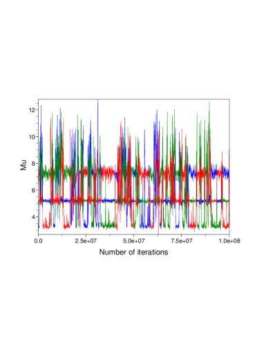
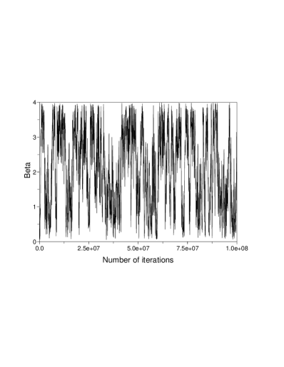
Figure 3: Trajectories over the $10^{8}$ first iterations of the ABF algorithm for the choice $\xi(\theta)=\beta$, for $(\mu_{1},\mu_{2},\mu_{3})$ (left) and for the $\beta$ variable (right).

Second, we monitor the convergence of the biasing potential. To this end, we run a simulation for a total number of iterations $T=10^{9}$, and store the biasing potential every $N_{\rm cvg}=10^{6}$ iterations. The distance between the current bias and the bias at iteration $t-N_{\rm cvg}$ is measured by

$$\delta_{t}=\sqrt{\inf_{c\in{\mathbb{R}}}\sum_{i=0}^{N_{z}-1}\left(A_{t,i}-A_{t-N_{\rm cvg},i}-c\right)^{2}},$$ (19)

where $A_{t,i}$ denotes the value of the bias in bin $i$, i.e. $A_{t}(z)=A_{t,i}$ if $z\in(z_{i},z_{i+1})$. Since the potential is defined only up to an additive constant, we consider the optimal shift constant $c$ which minimizes the mean-squared distance between the two profiles. An elementary computation shows that this constant is equal to the difference between the averages of $A_{t}$ and $A_{t-N_{\rm cvg}}$. We finally renormalize this distance as

$$\varepsilon_{t}=\frac{\delta_{t}}{\sqrt{\sum_{i=0}^{N_{z}-1}A_{t,i}^{2}}}.$$

The relative distance $\varepsilon_{t}$ as a function of the iteration index $t$ is plotted in Figure 4. Correct approximations of the bias are obtained after a few multiples of $N_{\rm cvg}$ iterations (the relative error being already lower than 0.1 at the first convergence check). We emphasize again that we did not optimize the proposal moves in order to reach the fastest convergence of the bias. It is very likely that better convergence results could be obtained by carefully tuning the parameters of the proposal function, or resorting to proposals of a different type.

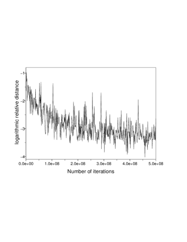
Figure 4: Convergence of the logarithmic relative distance $\log(\varepsilon_{t})/\log(10)$ (see (19)), as a function of the number of iterations.

On Figure 5, we plot the free energies associated to the four reaction coordinates mentioned above, as estimated by adaptive algorithms. We recall that, for $\xi(\theta)=\beta$, $z_{\rm min}=0.05$, $z_{\rm max}=4.0$ and $\Delta z=0.01$. For $\xi(\theta)=-\log\{p(\theta)p(y|\theta)\}$, we used an ABP algorithm, with $z_{\rm min}=500$, $z_{\rm max}=540$ and $\Delta z=0.1$. For $\xi(\theta)=q_{1}$ and $\xi(\theta)=\mu_{1}$, we used ABF, with respectively $z_{\rm min}=0$, $z_{\rm max}=1$, $\Delta z=0.005$ and $z_{\rm min}=\min y_{i}=2.5$, $z_{\rm max}=\max y_{i}=13$, $\Delta z=0.05$. Recall that the so-obtained bias is minus the marginal posterior log-density of $\xi$. This is why the three important modes in the $\mu$ parameter can be read from the corresponding bias in Figure 5. Note also that there is a lower bound on the admissible values of minus the log-posterior density, hence the plateau value of the corresponding bias for low values of the reaction coordinate corresponding to unexplored regions.

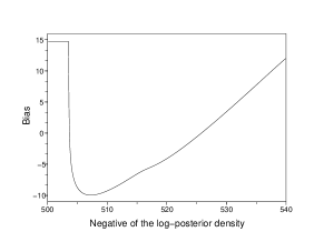
Figure 5: The fishery data. Free energies obtained for the reaction coordinates: $\xi(\theta)=\mu_{1}$ (top left), $\xi(\theta)=q_{1}$ (top right), $\xi(\theta)=\beta$ (bottom left) and $\xi(\theta)=-\log\{p(\theta)p(y|\theta)\}$ (bottom right).

5.1.2 Efficiency of the biasing procedure

We now discuss the results of the MCMC algorithm targeted at the biased posterior distribution, using the free energies computed above. In Figure 6, we observe that all the biased dynamics are much more successful in terms of mode switchings than the unbiased dynamics (see Figure 1). More precisely, the dynamics biased by the free energy associated with $\xi(\theta)=-\log\{p(\theta)p(y|\theta)\}$ is the most successful in terms of switchings, but the dynamics with $\xi(\theta)=\beta$ performs correctly as well. The dynamics with $\xi(\theta)=q_{1}$ seems to be less successful. In the case $\xi(\theta)=\mu_{1}$, one value of the parameters $\mu$ is forced to visit the whole range of values. The lowest mode (around $\mu=3$) is not very well visited here.

The efficiency factors are presented in Table 1. They are rather large, which shows that the importance sampling procedure does not yield a degenerate sample. The choice $\xi(\theta)=q_{1}$ is the best one, but $\xi(\theta)=\beta$ and $\xi(\theta)=-\log\{p(\theta)p(y|\theta)\}$ give comparable and satisfactory results as well. The choice $\xi(\theta)=\mu_{1}$ on the other hand is a poor choice in this case.

In view of these results, it seems that $\xi(\theta)=-\log\{p(\theta)p(y|\theta)\}$ is the best choice, with the problem however that we had to slightly modify the bias for the lowest values of the reaction coordinate because of the too sharp variations of the bias in this region. (Our numerical experience is indeed that the bias obtained from minus the log-posterior density is sometimes difficult to use directly.) On the other hand, the procedure is more automatic for $\xi(\theta)=q_{1}$ and $\beta$, the latter reaction coordinate being a much better choice when it comes to mode switchings.

Reaction coordinate	$\beta$	$-\log\{p(\theta)p(y|\theta)\}$	$q_{1}$	$\mu_{1}$
EF (numerical)	0.17	0.16	0.48	0.04
EF (theoretical)	0.179	0.178	0.454	0.079

Table 1: Efficiency factor for various choices of reaction coordinates, in the case $K=3$.

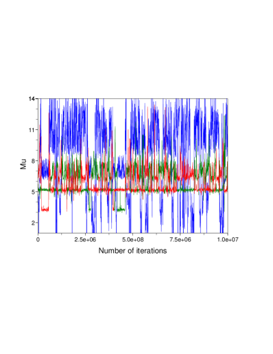
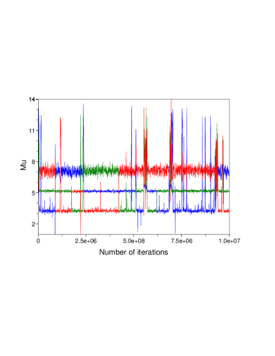
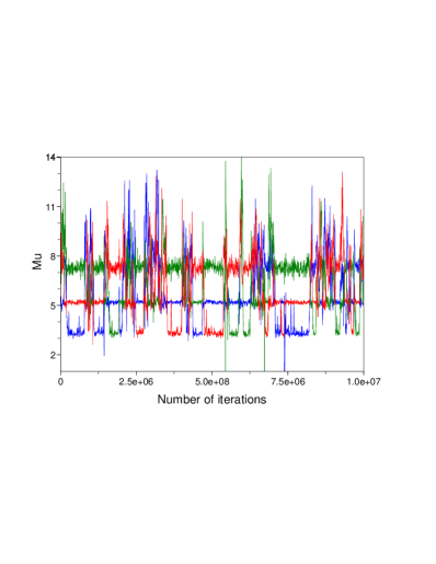
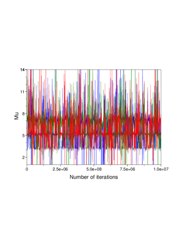
Figure 6: The fishery data. Trajectories of $(\mu_{1},\mu_{2},\mu_{3})$ for the biased dynamics for different reaction coordinates. Top left: $\xi(\theta)=\mu_{1}$. Top right: $\xi(\theta)=q_{1}$. Bottom left: $\xi(\theta)=\beta$. Bottom right: $\xi(\theta)=-\log\{p(\theta)p(y|\theta)\}$.

We now focus on $\xi(\theta)=\beta$. As explained in the introduction, a good sampler should visit all the possible labellings of the parameter space. This implies in particular that the marginal posterior distributions of the simulated component parameters should be nearly identical. This is clearly the case here, see the scatter plots of the 1-in-$10^{4}$ sub-sample of the simulated pairs $(\mu_{i},\log\lambda_{i})$, $i=1,\ldots,3$ in Figure 7. The top left picture in Figure 7 also demonstrates that the biased dynamics indeed samples uniformly the values of $\beta$ over the chosen interval $[z_{\rm min},z_{\rm max}]$.

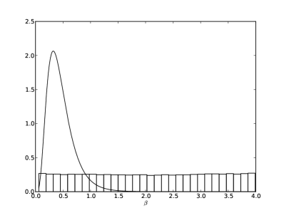
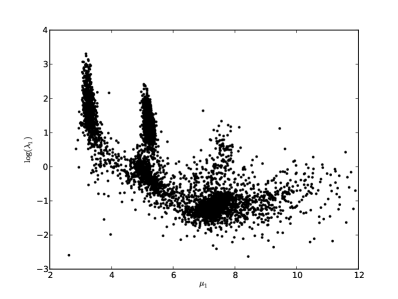
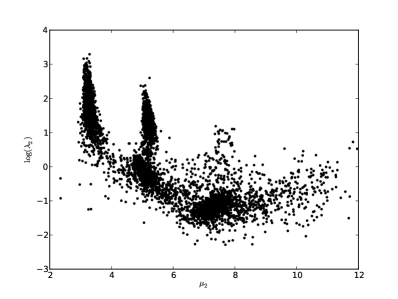
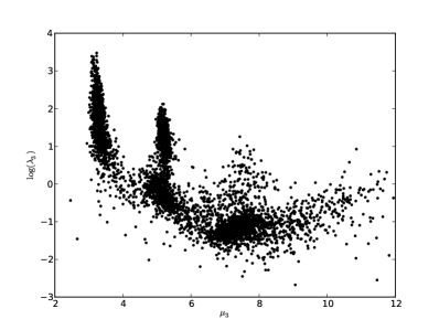
Figure 7: Top left: Histogram of simulated $\beta$’s and estimated marginal posterior density of $\beta$. Remaining pictures: Scatter plots of simulated values for $(\mu_{i},\log\lambda_{i})$, for $i=1,2,3$ when $\beta$ is used as a reaction coordinate.

Finally, Figure 8 illustrates why the reaction coordinate $\xi(\theta)=\beta$ allows for escaping from local modes; see the discussion in Section 4.2. Each plot represents a sub-sample of the simulated pairs $(\mu_{k,t},\log\lambda_{k,t})$ (where the subscript $t$ denotes the iteration index while the subscript $k$ labels the components), restricted to $\beta_{t}$ being in intervals, from left to right, $[0,0.5]$, $[1.5,2]$ and $[3.5,4]$. Since the bias function depends only on $\beta$, these plots are rough approximations of the posterior distribution conditional on $\beta=0.25$ (its posterior expectation), $\beta=1.75$ and $\beta=3$. In the leftmost plot of Figure 8, $\beta$ is fixed to its posterior expectation and the three modes are well separated. As $\beta$ is forced to take artificially large values (in the sense that the posterior probability density of such values is very small), the three modes get closer and eventually merge.

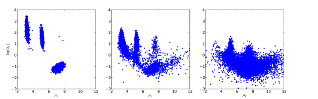
Figure 8: Simulated pairs $(\mu_{1},\log\lambda_{1})$ conditional on, from left to right, $\beta\in[0,0.5]$, $\beta\in[1.5,2]$ and $\beta\in[3.5,4]$, see Section 5.1.3 for more details.

5.1.3 Larger values of $K$ and model choice

We apply our approach to other values of $K$, namely $K=4$ to 6, in the case $\xi(\theta)=\beta$. Table 2 reports the efficiency factor as a function of $K$. These factors remain quite satisfactory, which is related to the fact that the amplitude of the free energy (difference between the maximum and the minimum values) associated to this reaction coordinate is not too large over the chosen interval $[z_{\rm min},z_{\rm max}]$, and does not change dramatically, see the profiles obtained for different values of $K$ in Figure 9.

$K$	3	4	5	6
EF (numerical)	0.17	0.18	0.17	0.16
EF (theoretical)	0.179	0.195	0.180	0.171

Table 2: Efficiency factors, for various values of the number of components considered in the mixture, with the choice $\xi(\theta)=\beta$.

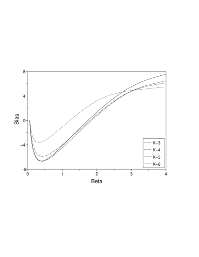
Figure 9: Estimated bias (free energy), for $K=3,\ldots,6$, and $\xi(\theta)=\beta$.

Figure 10 represents the marginal posterior distribution of $(\mu_{1},\log\lambda_{1})$, for $K=4,5,6$. These plots are obtained by resampling 2000 points from the output of the MCMC targeting the biased posterior, with probability proportional to the importance sampling weight defined in (14). In each case, we checked that the MCMC output is symmetric with respect to label permutations.

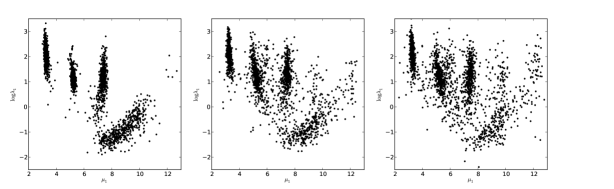
Figure 10: Marginal posterior distribution of $(\mu_{1},\log\lambda_{1})$, from left to right, for $K=4$, 5 and 6, as represented by 2000 points resampled from the MCMC output.

Table 3 reports, for $K=3,\ldots,6$, the estimated log-Bayes factor for choosing a mixture model with $K$ components against a mixture model with $K-1$ components, which equals $\log Z_{K}/Z_{K-1}$, assuming equal prior probability for different values of $K$. The reported error levels in Table 3 correspond to $90\%$ confidence intervals, which are deduced from repeated independent runs of $T=10^{7}$ iterations from the same MCMC algorithm targeting the biased posterior. The estimation error is quite small, despite being based on importance sampling steps in high dimensional spaces.

$K$	$\log Z_{K}/Z_{K-1}$	error
3	7.1	$\pm$ 0.2
4	4.2	$\pm$ 0.1
5	1.5	$\pm$ 0.1
6	0.9	$\pm$ 0.1

Table 3: Log Bayes factors for comparing model with $K$ components against $K-1$ components, for $K=3,...,6$; estimation error as evaluated from independent MCMC runs.

5.2 A second example: the Hidalgo stamps data

Another well-known benchmark for mixtures is the Hidalgo stamps dataset, first studied by Izenman and Sommer (1988) (see also e.g. Basford et al. (1997)), which consists of the thickness (in mm) of $n=485$ stamps from a given Mexican stamp issue; see Figure 1 for a histogram. (For convenience we multiplied the observations by 100.) We focus our presentation on the challenging case $K=3$. For other values of $K$ between 4 and 7 our approach performs better than for $K=3$. For the sake of space the corresponding results are not reported.

This example is more challenging than the previous one, presumably because the number of observations is larger, which makes the likelihood more peaked. A clear sign of the increasing metastability is the increase in the free-energy barriers. For the reaction coordinates $\xi(\theta)=q_{1}$, $\xi(\theta)=\beta$, $\xi(\theta)=-\log\{p(\theta)p(y|\theta)\}$, we had to run the adaptive algorithm for $T=10^{9}$ iterations in order to obtain a converged bias and recover a biased posterior sample which is symmetric by labelling. Again, a more elaborate proposal strategy for the Hastings-Metropolis step in the adaptive algorithm would be likely to stabilize the bias faster. As an illustration, Figure 11 presents the trajectories of $(\mu_{1},\mu_{2},\mu_{3})$ sampled by the adaptive algorithm, with random walk scales: $\tau_{q}=0.001$, $\tau_{\mu}=0.05$, $\tau_{v}=0.1$ and $\tau_{\beta}=0.005$. The trajectories should be compared to the ones depicted in Figure 1, which are obtained with the same proposal, but without any biasing procedure.

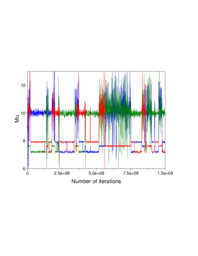
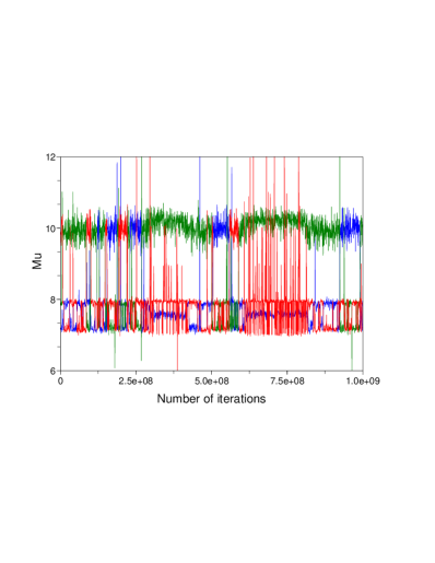
Figure 11: Sampled trajectories for $(\mu_{1},\mu_{2},\mu_{3})$ during the adaptive biasing procedure. Left: ABF trajectory when the reaction coordinate is $\beta$. Right: ABP trajectory when the reaction coordinate is minus the log-posterior density.

In Figure 12, we represent the biases obtained with various choices of the reaction coordinate. In the case $\xi(\theta)=\beta$, we set $z_{\rm min}=0.005$, $z_{\rm max}=2.5$ and $\Delta z=0.005$. For $\xi(\theta)=q_{1}$, we consider $z_{\rm min}=0$, $z_{\rm max}=1$ and $\Delta z=0.005$. Finally, for $\xi(\theta)=-\log\{p(\theta)p(y|\theta)\}$, we choose $z_{\rm min}=720$, $z_{\rm max}=780$ and $\Delta z=0.1$.

Figure 12: Hidalgo stamps problem. Free energies obtained for the reaction coordinates: $\xi(\theta)=q_{1}$ (top left), $\xi(\theta)=\beta$ (top right) and $\xi(\theta)=-\log\{p(\theta)p(y|\theta)\}$ (bottom).

Biased trajectories are presented in Figure 13 for $\xi(\theta)=q_{1}$, $\xi(\theta)=\beta$, and $\xi(\theta)=-\log\{p(\theta)p(y|\theta)\}$. Efficiency factors are reported in Table 4. The results show that, in terms of mode switching, $\xi(\theta)=-\log\{p(\theta)p(y|\theta)\}$ is the best choice. The choice $\xi(\theta)=q_{1}$, although it leads to the highest efficiency factor, is a poor choice since very few switchings are observed; in particular, the mode starting around 7.5 does not change during the first $2.5\times 10^{7}$ iterations. Such transitions are observed in the case $\xi(\theta)=\beta$.

Reaction coordinate	$\beta$	$-\log\{p(\theta)p(y|\theta)\}$	$q_{1}$
EF (numerical)	0.02	0.24	0.23
EF (theoretical)	0.06	0.13	0.18

Table 4: Efficiency factor for various choices of reaction coordinates, in the case $K=3$.

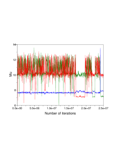
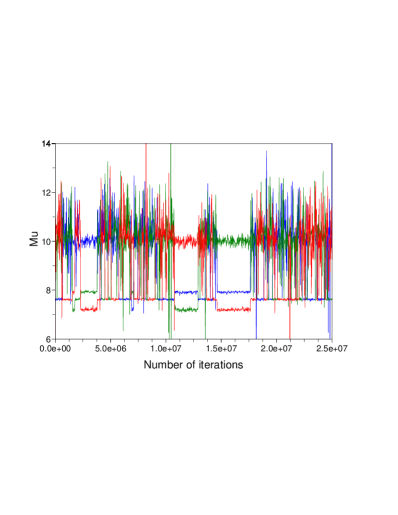
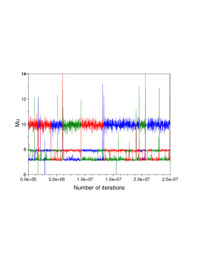
Figure 13: Hidalgo stamps problem. Trajectories of $(\mu_{1},\mu_{2},\mu_{3})$ of the biased dynamics. Top left: reaction coordinate $\xi(\theta)=q_{1}$. Top right: $\xi(\theta)=\beta$. Bottom: $\xi(\theta)=-\log\{p(\theta)p(y|\theta)\}$.

6 Conclusion

We showed in this paper how to sample efficiently posteriors of univariate Gaussian mixture models, using a free energy biasing approach, which can be summarized as follows:

1. We choose a reaction coordinate (a function $\xi$ of $\theta$).

2. We run an adaptive MCMC sampler, in order to compute an estimation of the free energy $A$ associated to $\xi$.

3. From the estimated free energy $\widehat{A}$ (the output of the previous step), we define the biased density $\widetilde{\pi}=\pi_{\widehat{A}}$. We run a standard MCMC sampler that targets $\widetilde{\pi}$ (say a Gaussian random-walk Hastings-Metropolis algorithm).

4. We do an importance sampling step, from $\widetilde{\pi}$ to $\pi$ to remove the bias and recover the true posterior $\pi$.

In the particular case of univariate Gaussian mixture models, a good choice for the reaction coordinate is $\xi=\beta$ or $\xi(\theta)=-\log\{p(\theta)p(y|\theta)\}$. When $\beta$ is chosen, it is easy to estimate an interval of typical values for $\beta$ as $[c_{1}R^{2},c_{2}R^{2}]$ (with $R$ the range of the data, and $c_{1}<c_{2}$ small constants, say $c_{1}=1/2000$ and $c_{2}=1/20$), while the determination of such an interval for $-\log\{p(\theta)p(y|\theta)\}$ does not seem to be straightforward.

We think that the same ideas may be applied to other mixture models. For instance, Figure 14 plots the posterior density of a two-component Poisson mixture model, conditional on different values for the hyper-parameters. Specifically, $p(y_{i}|\theta)=q_{1}\mathrm{Poisson}(y_{i};\lambda_{1})+(1-q_{1})\mathrm{Poisson}(y_{i};\lambda_{2})$ for $i=1,\ldots,n$, where $\mathrm{Poisson}(\cdot;\lambda)$ denotes the probability density function of a Poisson distribution of parameter $\lambda$. We use a $\mathrm{Gamma}(\beta\bar{y},\beta)$ prior for the $\lambda_{k}$’s, and a uniform prior for $q_{1}$. The $n=100$ observations are simulated from this model with parameters $(q_{1},\lambda_{1},\lambda_{2})=(0.7,3,10)$. It can be seen again that biasing the posterior distribution towards larger values of $\beta$ makes it possible to reduce the distance between the different modes. We also obtained interesting preliminary results for multivariate Gaussian mixtures.

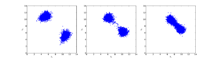
Figure 14: Scatter plots of 1000 simulated pairs $(\lambda_{1},\lambda_{2})$ from the posterior distribution of a two-component Poisson mixture model, and $n=100$ simulated data points, with a $\mathrm{Gamma}(\beta\bar{y},\beta)$ prior for the $\lambda_{k}$, and, from left to right, $\beta=1$, 10, 20.

We would like to highlight some practical advantages of our approach. First, it requires little tuning: The main tuning parameters are the scales of the random walks in both algorithms (adaptive, and MCMC), and we obtained satisfactory results without trying to optimize these scales. Second, it is easy to check that the final results are correct: If the free energy has been well estimated, and the MCMC algorithm for the biased posterior has converged, then a nearly uniform marginal distribution for the reaction coordinate is observed, and the marginal distributions for the $(\mu_{k},\lambda_{k},q_{k})$ are nearly identical, because of the symmetry of the true posterior, and the numerous mode switchings in the MCMC trajectories.

Finally, one natural question is how to extend such an approach to other classes of Bayesian models. As we have made clear already, the choice of the reaction coordinate is the crucial point. If the reaction coordinate is poorly chosen, a free energy biasing approach will bring no benefit. As for applications in computational Statistical Physics, there is no general recipe for choosing this reaction coordinate. Nonetheless, the following simple remarks may be considered as some guidelines. First, it seems worth investigating alternatives to the reaction coordinate usually chosen in Statistics, namely the negative of the posterior log-density. Second, in doing so, one may keep in mind the interpretation we proposed for $\xi(\theta)=\beta$ in Section 4.2, i.e. a particular parameter that fixes to some extent the size of the energy barriers between the different modes. In particular, in a given Bayesian hierarchical model, the hyper-parameters at the highest level of the hierarchy could be interesting candidates, because their values strongly influence the typical values of the other components of the system. More research in this direction is however required to draw more definite conclusions.

Acknowledgements

Part of this work was done while the two last authors were participating to the program “Computational Mathematics” at the Haussdorff Institute for Mathematics in Bonn, Germany. Support from the ANR grants ANR-008-BLAN-0218 and ANR-09-BLAN-0216 of the French Ministry of Research is acknowledged. The authors thank Julien Cornebise, Arnaud Doucet, Peter J. Green, Pierre Jacob, Christian P. Robert, Gareth Roberts, and the referees for insightful remarks.

References

- Ambrosio et al. (2000) L. Ambrosio, N. Fusco, and D. Pallara. Functions of Bounded Variation and Free Discontinuity Problems. Oxford Science Publications, 2000.
- Andrieu and Thoms (2008) C. Andrieu and J. Thoms. A tutorial on adaptive MCMC. Statist. Comput., 18(4):343–373, 2008.
- Atchadé and Liu (2010) Y. F. Atchadé and J. S. Liu. The Wang-Landau algorithm for Monte-Carlo computation in general state spaces. Stat. Sinica, 20(1):209–233, 2010.
- Balian (2007) R. Balian. From Microphysics to Macrophysics. Methods and Applications of Statistical Physics, volume I - II. Springer, 2007.
- Basford et al. (1997) K. E. Basford, G. J. Mclachlan, and M. G. York. Modelling the distribution of stamp paper thickness via finite normal mixtures: The 1872 Hidalgo stamp issue of Mexico revisited. J. Appl. Stat., 24(2):169–180, 1997.
- Bussi et al. (2006) G. Bussi, A. Laio, and M. Parrinello. Equilibrium free energies from nonequilibrium metadynamics. Phys. Rev. Lett., 96(9):090601, 2006.
- Celeux et al. (2000) G. Celeux, M. Hurn, and C. P. Robert. Computational and inferential difficulties with mixture posterior distributions. J. Am. Statist. Assoc., 95:957–970, 2000.
- Chipot and Lelièvre (2010) C. Chipot and T. Lelièvre. Enhanced sampling of multidimensional free-energy landscapes using adaptive biasing forces. arXiv preprint, 1008.3457, 2010.
- Darve and Pohorille (2001) E. Darve and A. Pohorille. Calculating free energies using average force. J. Chem. Phys., 115(20):9169–9183, 2001.
- Dickson et al. (2010) B.M. Dickson, F. Legoll, T. Leli vre, G. Stoltz, and P. Fleura-Lessard. Free energy calculations: An efficient adaptive biasing potential method. J. Phys. Chem. B, 114(17):5823–5830, 2010.
- Diebolt and Robert (1994) J. Diebolt and C. P. Robert. Estimation of finite mixture distributions through Bayesian sampling. J. R. Statist. Soc. B, 56:363–375, 1994.
- Evans and Gariepy (1992) L. C. Evans and R. F. Gariepy. Measure Theory and Fine Properties of Functions. Studies in Advanced Mathematics. CRC Press, 1992.
- Frühwirth-Schnatter (2006) S. Frühwirth-Schnatter. Finite Mixture and Markov Switching Models. Springer, 2006.
- Frühwirth-Schnatter (2001) S. Frühwirth-Schnatter. Markov chain Monte Carlo estimation of classical and dynamic switching and mixture models. J. Am. Statist. Assoc., 96(453):194–209, 2001.
- Gelman and Meng (1998) A. Gelman and X. L. Meng. Simulating normalizing constants: from importance sampling to bridge sampling to path sampling. Stat. Sci., 13(2):163–185, 1998.
- Hastings (1970) W. K. Hastings. Monte Carlo sampling methods using Markov chains and their applications. Biometrika, 57:97–109, 1970.
- Hénin and Chipot (2004) J. Hénin and C. Chipot. Overcoming free energy barriers using unconstrained molecular dynamics simulations. J. Chem. Phys., 121(7):2904–2914, 2004.
- Iba (2001) Y. Iba. Extended ensemble Monte Carlo. Int. J. Modern Phys. C, 12(5):623–656, 2001.
- Izenman and Sommer (1988) A. J. Izenman and C. J. Sommer. Philatelic mixtures and multimodal densities. J. Am. Stat. Assoc., 83(404):941–953, 1988.
- Jasra et al. (2005) A. Jasra, C. C. Holmes, and D. A. Stephens. Markov chain Monte Carlo methods and the label switching problem in Bayesian mixture modeling. Statist. Science, pages 50–67, 2005.
- Jourdain et al. (2010) B. Jourdain, T. Lelièvre, and R. Roux. Existence, uniqueness and convergence of a particle approximation for the Adaptive Biasing Force process. ESAIM-Math. Model. Num., 44(5):831–865, 2010.
- Kong et al. (1994) A. Kong, J. S. Liu, and W. H. Wong. Sequential imputation and bayesian missing data problems. J. Am. Statist. Assoc., 89:278–288, 1994.
- Lelièvre and Minoukadeh (2011) T. Lelièvre and K. Minoukadeh. Longtime convergence of an adaptive biasing force method: The bi-channel case. Arch. Ration. Mech. Anal., accepted, 2011.
- Lelièvre et al. (2007) T. Lelièvre, M. Rousset, and G. Stoltz. Computation of free energy profiles with parallel adaptive dynamics. J. Chem. Phys, 126:134111, 2007.
- Lelièvre et al. (2008) T. Lelièvre, M. Rousset, and G. Stoltz. Long-time convergence of an adaptive biasing force method. Nonlinearity, 21:1155–1181, 2008.
- Lelièvre et al. (2010) T. Lelièvre, M. Rousset, and G. Stoltz. Free Energy Computations: A Mathematical Perspective. Imperial College Press, 2010.
- Liang (2005) F. Liang. A generalized Wang-Landau algorithm for Monte-Carlo computation. J. Am. Stat. Assoc., 100(472):1311–1327, 2005.
- Liang (2010) F. Liang. Trajectory averaging for stochastic approximation MCMC algorithms. Ann. Stat., 38(5):2823–2856, 2010.
- Marin and Robert (2007) J. M. Marin and C. P. Robert. Bayesian core: a practical approach to computational Bayesian statistics. Springer Verlag, 2007.
- Marsili et al. (2006) S. Marsili, A. Barducci, R. Chelli, P. Procacci, and V. Schettino. Self-healing Umbrella Sampling: A non-equilibrium approach for quantitative free energy calculations. J. Phys. Chem. B, 110(29):14011–14013, 2006.
- McLachlan and Peel (2000) G.J. McLachlan and D. Peel. Finite mixture models. Wiley New York, 2000.
- Metropolis et al. (1953) N. Metropolis, A. W. Rosenbluth, M. N. Rosenbluth, A. H. Teller, and E. Teller. Equations of state calculations by fast computing machines. J. Chem. Phys., 21(6):1087–1091, 1953.
- Neal (2001) R. M. Neal. Annealed importance sampling. Statist. Comput., 11:125–139, 2001.
- Piana and Laio (2007) S. Piana and A. Laio. A bias-exchange approach to protein folding. J. Phys. Chem. B., 111(17):4553–4559, 2007.
- Raiteri et al. (2006) P. Raiteri, A. Laio, F. L. Gervasio, C. Micheletti, and M. Parrinello. Efficient reconstruction of complex free energy landscapes by multiple walkers metadynamics. J. Phys. Chem. B, 110(8):3533–3539, 2006.
- Richardson and Green (1997) S. Richardson and P. J. Green. On Bayesian analysis of mixtures with an unknown number of components. J. R. Statist. Soc. B, 59(4):731–792, 1997.
- Robert and Casella (2004) C. P. Robert and G. Casella. Monte Carlo Statistical Methods, 2nd ed. Springer-Verlag, New York, 2004.
- Titterington et al. (1986) D. M. Titterington, A. F. Smith, and U. E. Makov. Statistical Analysis of Finite Mixture Distributions. Wiley, 1986.
- Wang and Landau (2001a) F. G. Wang and D. P. Landau. Determining the density of states for classical statistical models: A random walk algorithm to produce a flat histogram. Phys. Rev. E, 64(5):056101, 2001a.
- Wang and Landau (2001b) F. G. Wang and D. P. Landau. Efficient, multiple-range random walk algorithm to calculate the density of states. Phys. Rev. Lett., 86(10):2050–2053, 2001b.