Abstract

In this paper we determine the velocity, the energy and estimate writhe and twist helicity contributions of vortex filaments in the shape of torus knots and unknots (toroidal and poloidal coils) in a perfect fluid. Calculations are performed by numerical integration of the Biot-Savart law. Vortex complexity is parametrized by the winding number $w$, given by the ratio of the number of meridian wraps to that of the longitudinal wraps. We find that for $w<1$ vortex knots and toroidal coils move faster and carry more energy than a reference vortex ring of same size and circulation, whereas for $w>1$ knots and poloidal coils have approximately same speed and energy of the reference vortex ring. Helicity is dominated by the writhe contribution. Finally, we confirm the stabilizing effect of the Biot-Savart law for all knots and unknots tested, that are found to be structurally stable over a distance of several diameters. Our results also apply to quantized vortices in superfluid ⁴He.

1 Introduction

The study of vortex filament motion in an ideal fluid, and in particular of vortex rings in presence or absence of periodic displacements of the vortex axis from the circular shape (Kelvin waves), dates back to the late 1800s [39, 38]. Despite its long history, this study is still an active area of research [20, 18, 15]. For example, the fact that upon large amplitude Kelvin waves vortex rings can slow down and even reverse their translational motion has been recognised only recently [22, 7]. Alongside the traditional interest for problems in classical fluid mechanics, additional interest is motivated by current work on superfluid helium [42, 9, 17, 13] and atomic Bose-Einstein condensates [41, 27, 19].

Here we shall be concerned with slightly more complex vortex structures; namely vortex filaments in the shape of torus knots and unknots in an ideal fluid. Since these vortices are closely related to circular vortex filaments with small-amplitude distortions lying on a mathematical torus, like vortex rings they propagate in the fluid by self-induction along the central axis of the torus, and they also rotate in their meridian plane (the poloidal plane of the torus) as their vortex core spins around the local center of mass, inducing an additional twisting motion of the vortex on itself, that cannot be neglected.

Among all possible knot types, torus knots constitute a special family of knots amenable to particularly simple mathematical description. These knots can be described by closed curves wound on a mathematical torus a number of times in the longitudinal direction of the torus and a number of times in the meridian direction. If these two numbers are co-prime integers greater than one, then we have standard torus knots (see Figure 1), whereas if the curve winds the torus only once in one of the two directions, then the curve is simply unknotted (see Figure 2), reducing to the standard circle when both numbers coincide with one. Even though torus unknots have trivial topology, their geometry may be rather complex, taking the shape of toroidal or poloidal coil, depending along which direction the curve is multiply wound.

Vortex torus knots and unknots provide a good example of structures that are relatively complex in space, but still amenable to study relationships between dynamical properties, like velocity and energy, and geometric and topological features, a step further towards the study of more complex structures present in turbulent flows. The aim of this paper is thus to continue and extend previous work [35, 26] to more complex vortex structures. Here we shall investigate the propagation velocity and the kinetic energy of vortex torus knots and unknots in some generality, by comparing results to a standard vortex ring of same size. Since superfluid ⁴He has zero viscosity, thus providing a realistic example of an Euler fluid, we shall choose circulation and vortex core radius as physically realistic quantities for quantized vortices in superfluid helium, and we shall carry out the research by direct numerical integration of the Biot-Savart law. Unlike previous vortex dynamics calculations of quantized vorticity [37, 1, 6, 40], however, we shall assume that no friction force [10] acts on the superfluid vortices; thus our results will apply to superfluid helium at temperatures below $1\leavevmode\nobreak\ \rm K$, where the dissipative effects of the normal fluid are truly negligible.

2 Mathematical background

2.1 Vortex motion under Biot-Savart and LIA law

We consider vortex motion in an ideal, incompressible fluid, in an unbounded domain. The velocity field ${\bf u}={\bf u}({\bf x},t)$, smooth function of the vector position ${\bf x}$ and time $t$, satisfies

$$\nabla\cdot{\bf u}=0\quad\textrm{in}\ {\hbox{I\kern-1.4pt{R}}}^{3}\ ,\qquad{\bf u}\to 0\quad\textrm{as}\ {\bf x}\rightarrow\infty\ ,$$ (1)

with vorticity $\omega$ defined by

$${\mbox{\boldmath$\omega$}}=\nabla\times{\bf u}\ ,\qquad\nabla\cdot{\mbox{\boldmath$\omega$}}=0\quad\textrm{in}\ {\hbox{I\kern-1.4pt{R}}}^{3}\ .$$ (2)

In absence of viscosity, fluid evolution is governed by the Euler equations and vortex motion obeys Helmholtz’s conservation laws [36]. Transport of vorticity is given by

$$\frac{\partial{\mbox{\boldmath$\omega$}}}{\partial t}=\nabla\times\left({\bf u}\times{\mbox{\boldmath$\omega$}}\right)\ ,$$ (3)

admitting formal solutions in terms of the Cauchy equations

$$\omega_{i}({\bf x},t)=\omega_{j}({\bf a},0)\frac{\partial x_{i}}{\partial{\rm a}_{j}}\ .$$ (4)

From this expression we can see how both convection of vorticity from the initial position ${\bf a}$ to the final position ${\bf x}$, and the simultaneous rotation and distortion of the vortex elements by the deformation tensor $\partial x_{i}/\partial{\rm a}_{j}$ are combined together. Since this tensor is associated with a continuous deformation of the vortex elements (by the diffeomorphism of the flow map), vorticity is thus mapped continuously from its initial configuration ${\mbox{\boldmath$\omega$}}({\bf a},0)$ to the final state given by ${\mbox{\boldmath$\omega$}}({\bf x},t)$; hence the Cauchy equations establish a topological equivalence between initial and final configuration by preserving vorticity topology. In absence of dissipation, physical properties such as kinetic energy, helicity and momenta are therefore conserved along with topological quantities such as knot type, minimum crossing number and self-linking number [33].

The kinetic energy per unit density $E$ is given by

$$E=\frac{1}{2}\int_{V}\|{\bf u}\|^{2}\,\rm d^{3}{\bf x}=constant\ ,$$ (5)

where $V=V$ is the fluid volume, and the kinetic helicity $H$ by

$$H=\int_{V}{\bf u}\cdot{\mbox{\boldmath$\omega$}}\,\rm d^{3}{\bf x}=constant\ .$$ (6)

Here we assume to have only one vortex filament ${\cal F}$ in isolation, where ${\cal F}$ is centred on the curve ${\cal C}$ of equation ${\bf X}={\bf X}(s)$ ($s$ being the arc-length of ${\cal C}$). The filament axis ${\cal C}$ is given by a smooth (that is at least $C^{2}$), simple (i.e. without self-intersections), space curve ${\cal C}$. The filament volume is given by $V({\cal F})=\pi a^{2}L$, where $L=L({\cal C})$ is the total length of ${\cal C}$ and $a$ is the radius of the vortex core, assumed to be uniformly circular all along ${\cal C}$ and much smaller than any length scale of interest in the flow (thin-filament approximation); this assumption is relevant (and particularly realistic) in the context of superfluid helium vortex dynamics, where typically $a\approx 10^{-8}\rm cm$.

Vortex motion is governed by the Biot-Savart law (BS for short) given by

$${\bf u}({\bf x})=\frac{\Gamma}{4\pi}\oint_{{\cal C}}\frac{{\hat{\bf t}}\times({\bf x}-{\bf X}(s))}{\|{\bf x}-{\bf X}(s)\|^{3}}\,\rm ds\ ,$$ (7)

where $\Gamma$ is the vortex circulation due to ${\mbox{\boldmath$\omega$}}=\omega_{0}{\hat{\bf t}}$, where $\omega_{0}$ is a constant and ${\hat{\bf t}}={\hat{\bf t}}(s)=\rm d{\bf X}/\rm ds$ the unit tangent to ${\cal C}$. Since the Biot-Savart integral is a global functional of vorticity and geometry, analytical solutions in closed form other than the classical solutions associated with rectilinear, circular and helical geometry are very difficult to obtain. Considerable analytical progress, however, has been done by using the Localized Induction Approximation (LIA for short) law. This equation, first derived by Da Rios [14] and independently re-discovered by Arms & Hama [4] (see the review by Ricca [30]), is obtained by a Taylor’s expansion of the Biot-Savart integrand from a point on ${\cal C}$ (see, for instance, the derivation by Batchelor [11]). By neglecting the rotational component of the self-induced velocity (that in any case does not contribute to the displacement of the vortex filament in the fluid) and non-local terms, the LIA equation takes the simplified form

$${\bf u}_{\rm LIA}=\frac{\Gamma c}{4\pi}\ln{\delta}\,{\hat{\bf b}}\propto c{\hat{\bf b}}\ ,$$ (8)

where $c=c(s)$ is the local curvature of ${\cal C}$, $\delta$ is a measure of the aspect ratio of the vortex, given by the radius of curvature divided by the vortex core radius) and ${\hat{\bf b}}={\hat{\bf b}}(s)$ the unit binormal vector to ${\cal C}$.

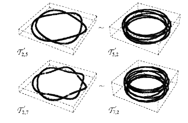
Figure 1: Examples of torus knots with winding number $w>1$ (left column) and $w<1$ (right column). Note that for given $p$ and $q$, torus knot ${\cal T}_{p,q}$ is topologically equivalent to the knot ${\cal T}_{q,p}$, and we write ${\cal T}_{p,q}\sim{\cal T}_{q,p}$. The tube centred on each knot is only for visualization purposes.

2.2 Torus knots

We consider a particular family of vortex configurations in the shape of torus knots in ${\hbox{I\kern-1.4pt{R}}}^{3}$. These are given when the curve ${\cal C}$ takes the shape of a torus knot ${\cal T}_{p,q}$ ($\{p,q\}$ co-prime integers with $p>1$ and $q>1$), given by a closed curve wound on a mathematical torus $p$ times in the longitudinal (toroidal) direction and $q$ times in the meridian (poloidal) direction (see Figure 1). When one of the integers is equal to one and the other is equal to $m$ the curve is no longer knotted, thus forming an unknot homeomorphic to the standard circle ${\cal U}_{0}$, but with a more complex geometry. Depending on which index takes the value $m$, the curve takes the shape of a toroidal coil ($p=m$) ${\cal U}_{m,1}$, or a poloidal coil ($q=1$) ${\cal U}_{1,m}$ (see Figure 2). When $\{p,q\}$ are both rational, ${\cal T}_{p,q}$ is no longer a closed knot, the curve covering the toroidal surface completely. Here we shall consider only curves given by $\{p,q\}$ integers. The ratio $w=q/p$ denotes the winding number and $Lk=pq$ the self-linking number, two topological invariants of ${\cal T}_{p,q}$. Note that for given $p$ and $q$ the knot ${\cal T}_{p,q}$ is topologically equivalent to ${\cal T}_{q,p}$, that is ${\cal T}_{p,q}\sim{\cal T}_{q,p}$, i.e. they are the same knot type, even though their geometry is completely different: toroidal coils resemble thick vortex rings with one full turn of twist of vorticity (internal swirl flow), whereas poloidal coils may recall circular jet flow generated by helicoidal distribution of vorticity on circular central axis.

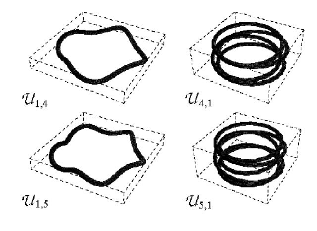
Figure 2: Examples of torus unknots with winding number $w>1$ (poloidal coils; left column) and $w<1$ (toroidal coils; right column). All these unknots are topologically equivalent to the standard circle. The tube centred on each unknot is shown only for visualization purposes.

A useful measure of geometric complexity of ${\cal C}$ is given by the writhing number [16] defined by

$$Wr\left({\cal C}\right)\equiv\frac{1}{4\pi}\oint_{{\cal C}}\oint_{{\cal C}}\frac{{\hat{\bf t}}(s)\times{\hat{\bf t}}(s^{\ast})\cdot[{\bf X}(s)-{\bf X}(s^{\ast})]}{\|{\bf X}(s)-{\bf X}(s^{\ast})\|^{3}}\,\rm ds\ \rm ds^{\ast}\ ,$$ (9)

where ${\bf X}(s)$ and ${\bf X}(s^{\ast})$ denote two points on the curve ${\cal C}$ for any pair $\{s,s^{\ast}\}\in\left[0,L\right]$, the integration being performed twice on the same curve ${\cal C}$. The writhing number provides a direct measure of coiling and distortion of the filament in space. This information can be related to the total twist $Tw$ and, by knowing the self-linking number $Lk$ of each knot, to the helicity $H$ of the vortex, that can be estimated to be $H=\Gamma Lk=\Gamma(Wr+Tw)$ [34], without resorting to direct calculation of the integral (6).

Now, let us identify each knot ${\cal T}_{p,q}$ with the vortex filament (we shall hereafter refer to ${\cal T}_{p,q}$ as the vortex torus knot), and consider dynamics and energy by using the BS (7) and the LIA law (8) to determine the effects of different geometries and topologies on dynamical properties and kinetic energy.

The existence of torus knot solutions to LIA were found by Kida [21] in terms of elliptic integrals. By re-writing LIA in cylindrical polar coordinates $(r,\alpha,z)$, and by using standard linear perturbation techniques, small-amplitude torus knot solutions (asymptotically equivalent to Kida’s solutions) were derived by Ricca [28]. These latter give solution curves explicitly in terms of the arc-length $s$, given by

$$\left\{\begin{array}[]{lcl}r=r_{0}+\epsilon\sin(w\phi)\ ,\\[5.69054pt] \alpha=\displaystyle{\frac{s}{r_{0}}+\frac{\epsilon}{wr_{0}}\cos(w\phi)}\ ,\\[5.69054pt] z=\displaystyle{\frac{t}{r_{0}}+\epsilon\left(1+\frac{1}{w^{2}}\right)^{1/2}\cos(w\phi)}\ ,\end{array}\right.$$ (10)

where $r_{0}$ is the radius of the torus circular axis and $\epsilon\ll 1$ is the inverse of the aspect ratio of the vortex. Since the LIA is related [30] to the one-dimensional Non-Linear Schrödinger Equation (NLSE), torus knot solutions (10) correspond to helical travelling waves propagating along the filament axis, with wave speed $\kappa$ and phase $\phi=(s-\kappa t)/r_{0}$. Vortex motion is given by a rigid body translation and rotation, with translation velocity $u=\dot{z}=u$ along the torus central axis and a uniform helical motion along the circular axis of the torus given by radial and angular velocity components $\dot{r}$ and $\dot{\alpha}$. In physical terms, these waves provide an efficient mechanism for the transport of kinetic energy and momenta throughout the fluid.

By using eqs. (10), Ricca [29] proved the following linear stability result:

Theorem 1

Let ${\cal T}_{p,q}$ be a small-amplitude vortex torus knot under LIA. Then ${\cal T}_{p,q}$ is steady and stable under linear perturbations if and only if $q>p$ ($w>1$).

This result provides a criterium for LIA stability of vortex knots, and it can be easily extended to inspect stability of torus unknots (i.e. toroidal and poloidal coils). This stability result has been confirmed for the knot types tested by numerical experiments [35]. Interestingly, LIA unstable torus knot were found to be stable under the BS law, due to the global induction effects of the vortex. This unexpected result has motivated further work and some current research which is still in progress.

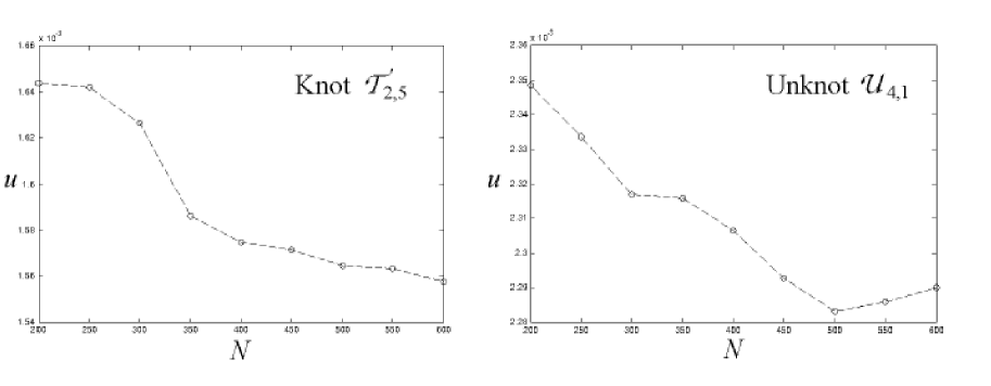
Figure 3: Examples of convergence test given by plots of the translational velocity $u$ against the number of discretization points $N$ on the vortex axis. Similar results have been found for the other knots/unknots tested. Broken lines are for visualization purposes only.

3 Numerical method

Dynamical quantities of vortex knots and unknots are evaluated by direct numerical integration of the BS law (7) and direct numerical calculation of the other properties. The numerical code is described in detail elsewhere [2] and it has been used also to study interaction and reconnection of vortex bundles [3]. The vortex axis is discretized into $N$ segments and the Biot-Savart integral is de-singularized by application of a standard cut-off technique [37, 1, 2]. The time evolution is realized by using a $4^{th}$ order Runge-Kutta algorithm. Convergence has been tested in space and time as usual by modifying the number of discretization points and the size of the time step.

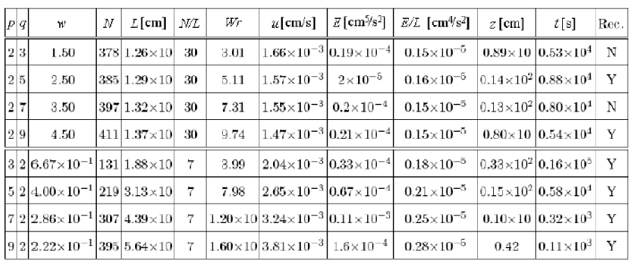
Figure 4: Vortex knots: numerical values of the calculated quantities. Entries in the last column report whether (Y) or not (N) a reconnection event has taken place on or before time $t$.

In all calculations, the initial condition is given by (10). We set $r_{0}=1\leavevmode\nobreak\ \rm cm$, $\epsilon=0.1$, $\Gamma=10^{-3}\leavevmode\nobreak\ \rm cm^{2}/s$, (the value expected for superfluid ⁴He), $\delta=2\times 10^{8}/e^{1/2}\gg 1$ (typical of a superfluid helium vortex core radius $a=10^{-8}\rm cm$). To analyse unknots we replace in eqs. (10) $(1-1/w^{2})$ with $|1-1/w^{2}|$. It is useful to compare these results with the dynamics of a vortex ring ${\cal U}_{0}$ of same size and vorticity. Thus we take a reference vortex ring with radius $r_{0}=1\leavevmode\nobreak\ \rm cm$. Typical time-step value in our calculations is $10^{-2}\leavevmode\nobreak\ \rm s$. Convergence in time has been tested by ranging the time-step from $10^{-3}\leavevmode\nobreak\ \rm s$ to $5\times 10^{-2}\leavevmode\nobreak\ \rm s$. Examples of convergence in space are shown in Figure 3 for torus knot $\mathcal{T}_{2,5}$ and unknot $\mathcal{U}_{4,1}$. The calculations are performed using constant mesh density $N/L$ chosen following convergence tests similar to those shown in Figure 3. We set $N/L=50$ for poloidal unknots $\mathcal{U}_{1,m}$ ($m=2,3,\ldots,7$), $N/L=20$ for toroidal unknots $\mathcal{U}_{m,1}$ ($m=2,3,\ldots,7$), $N/L=30$ for knots $\mathcal{T}_{2,q}$ ($q=3,5,7,9$) and $N/L=7$ for knots $\mathcal{T}_{p,2}$ ($p=3,5,7,9$). Typical errors in computing the velocity and the energy are approximately $10^{-5}\leavevmode\nobreak\ \rm cm/s$ and $10^{-7}\leavevmode\nobreak\ \rm cm^{5}/s^{2}$, respectively. For the reference vortex ring we set the winding number $w=1$ and $N=313$; then $L=6.26\leavevmode\nobreak\ \rm cm$, thus $N/L=50$, translational velocity $u_{0}=1.38\times 10^{-3}\leavevmode\nobreak\ \rm cm/s$, kinetic energy $E_{0}=8.77\times 10^{-6}\leavevmode\nobreak\ \rm\leavevmode\nobreak\ cm^{5}/s^{2}$ and obviously $H=0\leavevmode\nobreak\ \rm cm^{4}/s^{2}$.

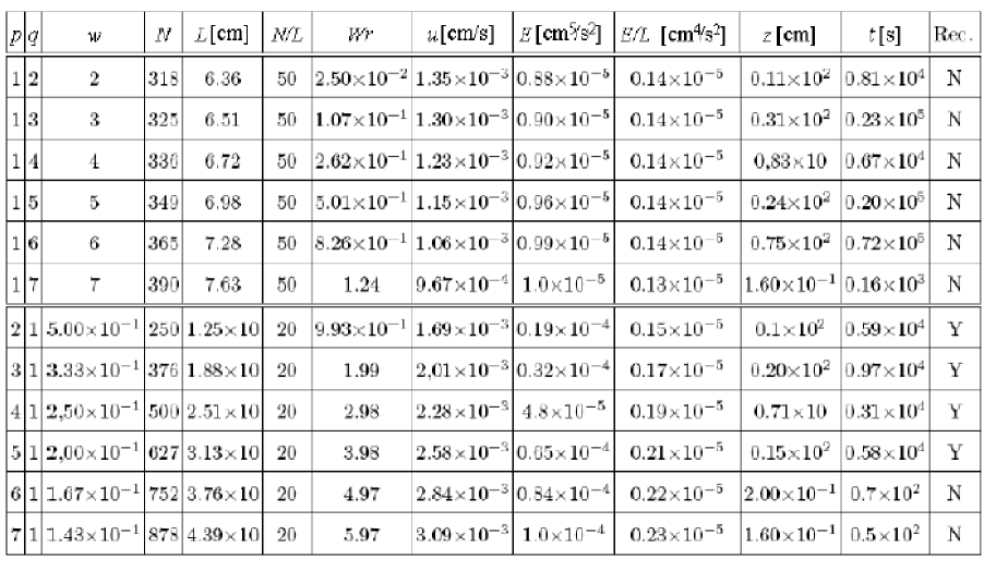
Figure 5: Vortex unknots: numerical values of the calculated quantities. Entries in the last column report whether (Y) or not (N) a reconnection event has taken place on or before time $t$.

4 Results: velocity, energy and helicity

Numerical values of calculated quantities are reported in the tables of Figure 4 and 5. Let us consider first purely geometric information, that will be useful to understand the following results on velocity, energy and helicity.

4.1 Total length and writhing number

Diagrams of total length and writhing of knots and unknots are shown in Figure 6. From diagrams of total length (left column), we see that these plots reflect the elementary fact that longitudinal wraps contribute to total length more than meridian wraps. The marked difference in the slope of the two plots in each diagram is just due to the dominant contribution to $L$ by the longitudinal wraps compared to the modest one of the meridian wraps. This behavior will be reflected in the relative kinetic energy of the system.

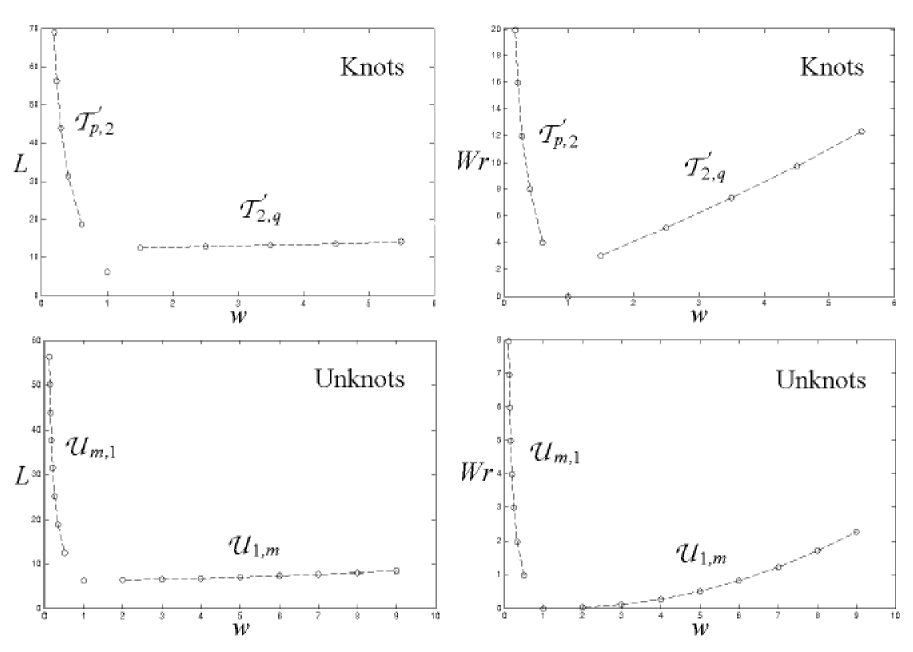
Figure 6: Total length $L$ and writhing number $Wr$ plotted against the winding number $w$ of the torus knots and unknots calculated ($p=3,5,7,9$; $q=3,5,7,9$; $m=2,3,\ldots,7$). The isolated circle denotes the reference vortex ring value. Broken lines are for visualization purposes only.

Similarly for the amount of coiling and distortion of the filament axis in relation to the dynamics and helicity of the vortex. As we can see from the diagrams on the right of Figure 6, meridian wraps contribute modestly (if not at all appreciably to our degree of accuracy) to the total writhing of the filament, the dominant contribution coming from the longitudinal wraps present. Moreover, since the self-linking of the vortex filament is a topologically conserved quantity [34] given by $Lk=Wr+Tw$, where $Tw$ denotes total twist of the filament, then information on writhing provides direct information on total twist, by taking $Tw=Lk-Wr$. Furthermore, being the number of meridian wraps directly proportional to total twist, we have an immediate estimate of the relative contributions to helicity (see the discussion in the sub-section below).

4.2 Translation velocity

The translational velocity $u=\dot{z}$ along the central axis of knots and unknots is calculated by using the Biot-Savart law. Absolute values are reported in the tables of Figure 4 and 5. The diagrams of Figure 7 show the normalized velocity $u/u_{0}$ of knots and unknots plotted against the winding number. The velocity is greatly influenced by the relative number of longitudinal wraps, which contribute greatly to the total curvature of the vortex. In general the velocity decreases with increasing winding number. Fastest vortex systems are thus torus knots with highest number of longitudinal wraps. In the case of unknots we can see that meridian wraps actually slow down poloidal coils ${\cal U}_{1,m}$, making them traveling slower than the corresponding vortex ring. At very high winding number, torus knots and poloidal coils seem to reverse their velocity, thus traveling backward in space. This curious phenomenon has been observed independently [22, 7], and it can be justified on theoretical grounds by information based on structural complexity analysis [31, 32].

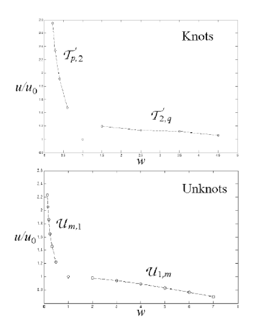
Figure 7: Translational velocity $u$ normalized with respect to the velocity $u_{0}$ of a reference vortex ring plotted against the winding number $w$ of the torus knots and unknots calculated ($p=3,5,7,9$; $q=3,5,7,9$; $m=2,3,\ldots,7$). The isolated circle denotes the reference vortex ring value. Broken lines are for visualization purposes only.

An estimate of the relationship between normalized velocity $u/u_{0}$ and winding number $w$ of torus knots is obtained by a linear regression, given by:

$$u/u_{0}=\left\{\begin{array}[]{l}4.41-9.13w+7.09w^{2}\ ,\qquad(w<1)\ ,\\[2.84526pt] 1.25-0.04w\ ,\qquad(w>1)\ ,\end{array}\right.$$ (11)

with standard deviation of 0.031.

In the limit $w\to 0$, the knot covers the toroidal surface completely with an infinite number of longitudinal wraps, and vorticity becomes a sheet of toroidal vorticity, with the induced velocity, purely poloidal in the interior and exterior region of the torus, that jumps across the sheet in opposite directions. The regression (11) suggests a theoretical limit value $u/u_{0}=4.41$ that seems to be independent of the aspect ratio of the torus. In the other limit, $w\to\infty$, the knot covers the torus with an infinite number of meridian wraps, and in this case vorticity induces a toroidal jet in the interior region.

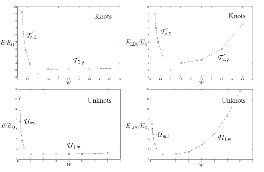
Figure 8: Left column: kinetic energy $E$ calculated by using the Biot-Savart law and normalized with respect to the energy $E_{0}$ of the reference vortex ring, plotted against the winding number $w$ of the knots and unknots calculated ($p=3,5,7,9$; $q=3,5,7,9$; $m=2,3,\ldots,7$). Right column: kinetic energy $E_{\rm LIA}$ calculated by using the LIA law and normalized with respect to the energy $E_{0}$ plotted against $w$. The isolated circle denotes the reference vortex ring value. Broken lines are for visualization purposes only.

4.3 Kinetic energy

The diagrams of the normalized kinetic energy per unit density $E/E_{0}$ (Figure 8, left column) of the knots and unknots calculated by using the Biot-Savart law, and the normalized energy calculated by the LIA law $E_{\rm LIA}/E_{0}$ (Figure 8, right column), plotted against the winding number $w$, show trends dictated by the behavior of total length $L=L(w)$ (cf. the diagrams of Figure 6). Here the calculation of the volume integral (5) is replaced by the more economical line integral [8]

$$E=\frac{\Gamma}{2}\oint_{{\cal C}}{\bf u}\cdot{\bf X}\times{\hat{\bf t}}\,\rm ds\ .$$ (12)

An estimate of the relationship between the normalized energy $E/E_{0}$ of torus knots and their winding number $w$ is given by a non-linear regression based on least squares:

$$E/E_{0}=2.35+67.03e^{-6.44w}\ ,\qquad(w<1)\ ,$$ (13)

with root mean square deviation of 0.218.

Different trends and values are obtained by calculating the normalized energy by using the LIA law; in this case, by using (8), we have

$$E_{\rm LIA}=\frac{1}{2}\int_{V}\|{\bf u}_{\rm LIA}\|^{2}\,\rm d^{3}{\bf x}=\left(\frac{\Gamma\ln\delta}{4\pi}\right)^{2}\oint_{{\cal C}}c^{2}\,\rm ds\ ,$$ (14)

that is one of the conserved quantities associated with the LIA law [28]. Direct comparison between the diagrams of the two energies reveals two distinct trends: for $w<1$ the LIA law under-estimates the actual energy of the vortex (knotted or unknotted), whereas for $w>1$ the LIA provides much higher energy values. The importance of non-local effects is evident: the LIA energy of ${\cal T}_{9,2}$ and ${\cal U}_{7,1}$, for example, is about 40% less than the corresponding BS energy, whereas ${\cal T}_{2,9}$ and ${\cal U}_{1,7}$ under LIA have 3 and 14 times more energy than their corresponding BS counterparts. These differences are essentially due to the contributions from the induction effects of nearby strands, captured by the BS law, but completely neglected under LIA.

Another quantity of interest is the kinetic energy per unit length $E/L$. From the tables of Figures 4 and 5 we see that for $w<1$ $E/L$ can vary by up to 100%. This result has interesting implications for the interpretation of experiments on superfluid turbulence, particularly at low temperatures, a regime that is dominated by Kelvin waves [24]. What is measured in the experiments is the total vortex length per unit volume $\Lambda$, and the turbulence energy per unit volume is deduced by multiplying the observed vortex length per volume times the energy per unit length; by integrating the velocity field of a straight vortex filament, the energy per unit length is estimated as $E/L\approx\Gamma^{2}/(4\pi^{2})\ln{(b/a)}$, where $b\approx\Lambda^{-1/2}$ is the typical distance between vortices. Our results show that for highly bent vortex filaments (as in the case of superfluid turbulence, where vorticity is even fractal [23]), $E/L$ is certainly not constant.

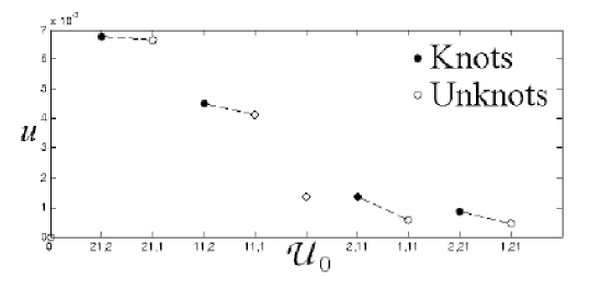
Figure 9: Translational velocity $u$ of some knots and related unknots reported here for comparison. In general knots travel faster than their corresponding unknots. The isolated circle denotes the reference vortex ring value. Broken lines are for visualization purposes only.

4.4 Helicity

It is interesting to investigate the effects of topology on the velocity and kinetic helicity, by exploring the interplay of geometric and topological aspects on the dynamics. For this let us consider Figure 9, where the velocities of a torus knot and that of the corresponding unknot with same number of longitudinal or meridian wraps are shown for comparison. As we see in general vortex knots travel faster than their corresponding unknots, and the higher the number of longitudinal wraps the faster is the motion, whereas the higher the number of meridian wraps the slower is the propagation speed.

As far as helicity is concerned, we have $H=\Gamma Lk$ [34] and for torus knots we can set $Lk=pq$, that is invariant for each knot type ($Tw$ being the total twist) and it increases with knot complexity. Since $Lk=Wr+Tw$ from the $Wr$-values of the table of Figure 4 we can compute $Tw$ for each knot. In general twist helicity is larger for knots with higher number of meridian wraps. For the unknots we can set $Lk=Wr+Tw=0$ (for the reference vortex ring we have zero writhe and zero twist); thus from the values of the table of Figure 5, we have $Tw=-Wr$ and therefore we can estimate writhe and twist helicity contributions.

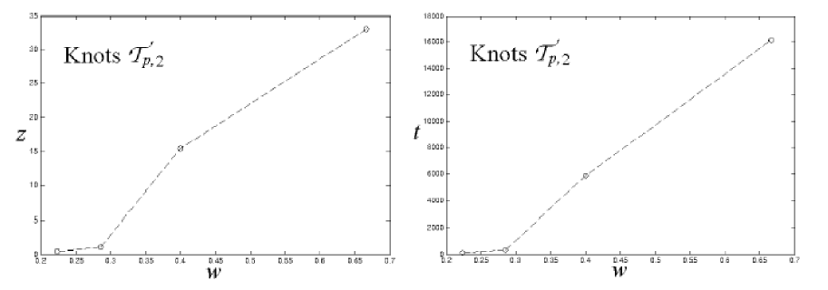
Figure 10: Plots of space travelled ($z$) and time elapsed ($t$) before a reconnection event takes place for torus knots ${\cal T}_{p,2}$ ($p=3,5,7,9$) plotted against the winding number $w$. Calculations are based on the Biot-Savart law. Broken lines are for visualization purposes only.

4.5 Structural stability considerations

Aspects of structural stability of vortex knots and unknots based on permanence of knot signature and occurrence of a reconnection event are explored. In previous work we noticed the stabilizing effect of the BS law on LIA-unstable knots [35]. Here we extend this comparison to the knots and unknots considered so far. In general a vortex structure is said to be stable if it evolves under signature-preserving flows that conserve topology, geometric signature and vortex coherency. Let us consider results reported in the tables of Figure 4 and 5 and shown in Figure 10.

Since our results concern both Euler’s and superfluid dynamics, it is important to remark that superfluid vortices can reconnect with each other in absence of dissipation [25, 12], whereas in the Euler context vortex topology is conserved; this important difference has been recently reviewed by Barenghi [5]. Here we adopt the following criterium: when, during the evolution, a vortex reconnection takes place, then we stop the calculation, and deem the structure to be unstable. The last column of the table of Figure 4 and 5 refers to the occurrence of a reconnection at instant $t$. In the absence of reconnection, we report the distance $z$ travelled by the vortex during the computational time $t$. If $z$ is much larger than the typical vortex size, the knot/unknot tested is said to be structurally stable.

From the last two columns of Figure 4 we see that for $w<1$ the space travelled tends to decrease with increasing knots complexity; for example, $t({\cal T}_{3,2})\gg t({\cal T}_{9,2})$. The effect is also shown in Figure 10. Note that these knots would be LIA-unstable. Thus, the stabilizing effect due to the BS law is confirmed: these knots can indeed travel a distance which is larger than their size before unfolding and reconnecting.

5 Conclusions

In this paper we examined the effect of several geometric and topological aspects on the dynamics and energetics of vortex torus knots and unknots (i.e. toroidal and poloidal coils). This study is carried out by numerically integrating the Biot-Savart law, and by comparing results for several knots and unknots at different winding numbers $w$. Generic behaviors are found for the class of knots/unknots tested, and main results are presented by normalizing velocity and energy by the corresponding value of a standard vortex ring (${\cal U}_{0}$) of same size and circulation.

In general, for $w<1$ (where the number of longitudinal wraps is larger than that of meridian wraps) the more complex the vortex structure is, the faster it moves, and both torus knots and toroidal coils move faster than ${\cal U}_{0}$. For $w>1$ (where the relative number of meridian wraps dominates) all vortex structures move essentially as fast as ${\cal U}_{0}$, almost independently from their total twist. Therefore, for all the structures tested total twist provides only a second-order effect on the dynamics.

We have also found that for $w<1$ vortex structures carry more kinetic energy than ${\cal U}_{0}$, whereas for $w>1$ knots and poloidal coils have almost the same energy as ${\cal U}_{0}$. The LIA law (an approximation often used to replace the Biot-Savart law, more computationally demanding) under-estimates the energy of knots with $w<1$ and over-estimate the energy for $w>1$.

Kinetic helicity, that is naturally decomposed in writhe and twist contributions, is evidently determined by the relative number of longitudinal and meridian wraps present, the latter contributing to twist helicity rather modestly (relatively).

Finally, we can extend previous results and confirm that for $w<1$ the Biot-Savart law has a stabilizing effect on knots that are LIA-unstable: all vortex structures tested have been found to be structurally stable regardless of the value of $w$, being able to travel in the fluid for several diameters before eventually unfolding and reconnecting.

References

- [1] R.G.K. Aarts & A.T.A.M. deWaele, Phys. Rev. B 50, 10069 (1994).
- [2] S.Z. Alamri, Ph.D. Thesis, Newcastle University (2009).
- [3] S.Z. Alamri, A.J. Youd & C.F. Barenghi, Phys. Rev. Lett. 101, 215302 (2008).
- [4] R.J. Arms. & F.R. Hama, Phys. Fluids 8, 553 (1965).
- [5] C.F. Barenghi, Physica D 237, 2195 (2008).
- [6] C.F. Barenghi, G.G. Bauer, D.C. Samuels & R.J. Donnelly, Phys. Fluids 9, 2631 (1997).
- [7] C.F. Barenghi, R. Hanninen & M. Tsubota, Phys. Rev. E 74, 046303 (2006).
- [8] C.F. Barenghi, R.L. Ricca & D.C. Samuels, Physica D 157, 197 (2001).
- [9] C.F. Barenghi & Y.A. Sergeev, Phys. Rev. B 80, 024514 (2009).
- [10] C.F. Barenghi, W.F. Vinen & R.J. Donnelly, J. Low Temp. Physics 52, 189 (1982).
- [11] G.K. Batchelor, An Introduction to Fluid Dynamics, Cambridge University Press (1967).
- [12] G.P. Bewley, M.S. Paoletti, K.R. Sreenivasan & D.P. Lathrop, Proc. Nat. Acad. Sci., 105, 13707 (2008).
- [13] G.P. Bewley & K.R. Sreenivasan, J. Low Temp. Phys. 156, 1573 (2009).
- [14] L.S. Da Rios, Rend. Circ. Mat. Palermo 22, 117 (1905).
- [15] Y. Fukumoto & H.K. Moffatt, Physica D 237, 2210 (2008).
- [16] F.B. Fuller, Proc. Nat. Acad. Sci. U.S.A. 68, 815 (1971).
- [17] A.I. Golov & P.M. Walmsley, J. Low Temp. Physics 156, 51 (2009).
- [18] Y. Hattori & Y. Fukumoto, Phys. of Fluids 21, 014104 (2009).
- [19] T.-L. Horng, C.-H. Hsueh, & S.-C. Gou, Phys. Rev. A 77, 063625 (2008).
- [20] F. Kaplanski, S.S. Sazhin & Y. Fukumoto, J. Fluid Mech. 662, 233 (2009).
- [21] S. Kida, J. Fluid Mech. 112 397 (1981).
- [22] L. Kiknadze & Yu. Mamaladze, J. Low temp. Phys. 124, 321 (2002).
- [23] D. Kivotides, C.F. Barenghi & D.C. Samuels, Phys. Rev. Lett. 87, 155301 (2001).
- [24] D. Kivotides, J.C. Vassilicos, D.C. Samuels & C.F. Barenghi, Phys. Rev. Lett. 86, 3080 (2001).
- [25] J. Koplik & H. Levine, Phys. Rev. Lett. 71, 1375 (1993).
- [26] F. Maggioni, S.Z. Alamri, C.F. Barenghi & R.L. Ricca, Il Nuovo Cimento C 32 133 (2009).
- [27] P.M. Mason & N.G. Berloff, Phys. Rev. A 79, 043620 (2009).
- [28] R.L. Ricca, Chaos 3, 83 (1993). [Also Erratum, Chaos 5, 346 (1995).]
- [29] R.L. Ricca, in Small-Scale Structures in Three-Dimensional Hydro and Magnetohydrodynamics Turbulence edited by M. Meneguzzi et al., 99 (1995), Lecture Notes in Physics 462. Springer-Verlag, Berlin.
- [30] R.L. Ricca, Fluid Dyn. Res. 18, 245 (1996).
- [31] R.L. Ricca, Physica D 237, 2223 (2008).
- [32] R.L. Ricca, in Lectures on Topological Fluid Mechanics edited by R.L. Ricca, 169 (2009), Springer-CIME Lecture Notes in Mathematics 1973. Springer-Verlag, Berlin.
- [33] R.L. Ricca & M.A. Berger, Phys. Today 12, 28 (1996).
- [34] R.L. Ricca & H.K. Moffatt, in Topological Aspects of the Dynamics of Fluids and Plasmas edited by H.K. Moffatt et al., 225 (1992), Kluwer, Dordrecht.
- [35] R.L. Ricca, D.C. Samuels & C.F. Barenghi, J. Fluid Mech. 29, 391 (1999).
- [36] P.G. Saffman, Vortex Dynamics Cambridge University Press (1992).
- [37] K.W. Schwarz, Phys. Rev. B 38, 2398 (1988).
- [38] J.J. Thomson, A treatise on the motion of vortex rings, MacMillan and Co. London (1883).
- [39] W. Thomson, Phil. Mag. 10 155 (1880).
- [40] M. Tsubota, C.F. Barenghi & T. Araki, J. Low Temp. Phys. 134, 471 (2004).
- [41] M. Tsubota & M. Kobayashi, J. Low Temp. Phys. 150, 402 (2008).
- [42] P.M. Walmsley, A.I. Golov, H.E. Hall, A.A. Levchenko & W.F. Vinen, Phys. Rev. Lett. 99, 265302 (2007).