RANDOM WALKS ESTIMATE LAND VALUE IN CITIES

Abstract

Expected urban population doubling calls for a compelling theory of the city. Random walks and diffusions defined on spatial city graphs spot hidden areas of geographical isolation in the urban landscape going downhill. First–passage time to a place correlates with assessed value of land in that. The method accounting the average number of random turns at junctions on the way to reach any particular place in the city from various starting points could be used to identify isolated neighborhoods in big cities with a complex web of roads, walkways and public transport systems.

1 The problem of massive urbanization

Multiple increases in urban population that had occurred in Europe at the beginning of the $20^{\mathrm{th}}$ century made urban agglomerations suffer from the problems of urban decay such as wide-spread poverty, high unemployment, and rapid changes in the racial composition of neighborhoods. Riots and social revolutions happened in response to conditions of urban decay in many European countries established regimes affecting immigrants and certain population groups de facto alleviating the burden of the haphazard urbanization by increasing its deadly price.

More than half of world’s population, 3.3 billion people, is now living in cities, and the figure is about to double by 2030 [1]. Urban sprawl in US covered $41,000$ $\mathrm{km}^{2}$ in 20 years, the area that equals that of the state of Switzerland [2]. In Europe, urban sprawl has covered $8,000$ $\mathrm{km}^{2}$ in 10 years the area that equals the territory of Luxembourg [3]. Unsustainable pressure on resources causes the increasing loss of fertile lands through degradation and climate changes through the increasing carbon emissions warming the earth’s atmosphere. City development planners will face great challenges in preventing cities from unlimited expansion.

Global poverty is in flight becoming a primarily urban phenomenon in the developing world. 2 billion new urban settlers in the next 20 years will live in slums on no more than $1 a day, adding to 1 billion already living there [4]. Faults in urban planning, poverty, redlining, immigration restrictions and clustering of minorities dispersed over the spatially isolated pockets of streets trigger urban decay, a process by which a city falls into a state of disrepair. The speed and scale of urban growth in that require urgent global actions to help cities prepare for growth and to avoid them of being the future epicenters of poverty and human suffering.

2 The scope of study and conclusions

In the present paper, we investigate spatial graphs of several compact urban patterns: the city canal networks of Venice and Amsterdam, as well as the almost regular array of streets in Manhattan.

In the next section (Sec. 3), we briefly discuss the principles which is are used for encoding urban environments into geometrical graphs. In Sec. 4, we develop the theory of linear automorphisms for undirected graphs and demonstrate that they can be interpreted as random walks on graphs. By the way, many geometrical properties of graph may acquire probabilistic interpretations. In particular, we are interested in first–passage times to the nodes of graphs – the expected number of steps required for random walkers starting from an arbitrary node of the graph to reach the given node for the first time. The first-passage time is the important characteristic of the node quantifying its isolation in the complex graph structure.

Sociologists think that isolation worsens an area’s economic prospects by reducing opportunities for commerce, and engenders a sense of isolation in inhabitants, both of which can fuel poverty and crime. It is well known that many social variables demonstrate striking spatial distribution patterns, and therefore may be detected and predicted by a structural analysis. In the last Sec. 5, we discuss two examples of such a type: the spatial isolation of Venetian Ghetto, the small area of Venice in which Jewish people were compelled to live under the Venetian Republic, and the value of land in the urban pattern of Manhattan. In particularly, we compare the tax assessment rates of places in Manhattan with first-passage times to them. The data positively relate the geographic accessibility of places in Manhattan with their ’unearned increments’ quantifying the level of appreciation in value of the site.

The proposed method could be used to identify isolated neighborhoods in big cities with a complex web of roads, walkways and public transport systems.

3 Spatial networks of urban environments

In traditional urban researches, the dynamics of an urban pattern come from the landmasses, the physical aggregates of buildings delivering place for people and their activity. The relationships between certain components of the urban texture are often measured along streets and routes considered as edges of a planar graph, while the traffic end points and street junctions are treated as nodes. Such a primary graph representation of urban networks is grounded on relations between junctions through the segments of streets. The usual city map based on Euclidean geometry can be considered as an example of primary city graphs.

In space syntax theory (see [5, 6]), built environments are treated as systems of spaces of vision subjected to a configuration analysis. Being irrelevant to the physical distances, spatial graphs representing the urban environments are removed from the physical space. It has been demonstrated in multiple experiments that spatial perception shapes peoples understanding of how a place is organized and eventually determines the pattern of local movement, [6]. The aim of the space syntax study is to estimate the relative proximity between different locations and to associate these distances to the densities of human activity along the links connecting them, [7, 8, 9]. The surprising accuracy of predictions of human behavior in cities based on the purely topological analysis of different urban street layouts within the space syntax approach attracts meticulous attention [10].

The decomposition of urban spatial networks into the complete sets of intersecting open spaces can be based on a number of different principles. In [11], while identifying a street over a plurality of routes on a city map, the named-street approach has been used, in which two different arcs of the primary city network were assigned to the same identification number (ID) provided they share the same street name.

In our paper, we take a ”named-streets”-oriented point of view on the decomposition of urban spatial networks into the complete sets of intersecting open spaces following our previous works [12, 13]. Being interested in the statistics of random walks defined on spatial networks of urban patterns, we assign an individual street ID code to each continuous segment of a street. The spatial graph of urban environment is then constructed by mapping all edges (segments of streets) of the city map shared the same street ID into nodes and all intersections among each pair of edges of the primary graph into the edges of the secondary graph connecting the corresponding nodes.

4 Theory of linear automorphisms for undirected graphs

4.1 Graphs and their linear automorphisms

Consider a transitive permutation group $\mathcal{P}(V)$ defined on a finite ordered set of objects $V$, $|V|=N$. Its representation consists of all $N\times N$ orthogonal matrices ${\bf\Pi}_{\sigma}$ such that $\left({\bf\Pi}_{\sigma}\right)_{i,\,\sigma i}=1$, and $\left({\bf\Pi}_{\sigma}\right)_{i,j}=0$ if $j\neq\sigma i$. We can define an induced action of $\mathcal{P}(G)$ on the set of all 2-subsets $V\times V$ by

$$\sigma(v,w)\,=\,\left(\sigma v,\sigma w\right),\quad\sigma\in\mathcal{P}(V),\quad v,w\in V.$$ (1)

Given a binary relation of adjacency ”$\sim$” defined on the finite set $V$, we denote its graph by $G$ and conveniently represent by its adjacency matrix $\bf A$ – the $N\times N$ matrix where the non-diagonal entry $A_{ij}=1$ if and only if $i\sim j$, and is zero otherwise.

Among all possible permutation groups $\mathcal{P}(V)$ defined over the set $V$, there is one ’compatible’ with the binary relation ”$\sim$” that is the automorphism group of the graph $\mathrm{Aut}(G)$ such that for any $\sigma\in\mathrm{Aut}(G)$, $u\sigma\sim v\sigma$, if and only if $u\sim v$. A permutation $\sigma\in\mathrm{Sym}(G)$ belongs to $\mathrm{Aut}(G)$ if and only if its matrix representation $\Pi_{\sigma}$ commutes with the adjacency matrix of $G$ [14],

$$\left[{\bf A},{\bf\Pi}_{\sigma}\right]\,=\,0.$$ (2)

A linear function of the graph $G$ defined on its adjacency matrix,

$$f\left({\bf A}\right)_{ij}\,=\,\sum_{\,s,l=1}^{N}\,F_{ij,sl}\,A_{sl},\quad F_{ij,sl}\,\in\,\mathbb{R},$$ (3)

belongs to the representation of the automorphism group $\mathrm{Aut}(G)$ in the group of linear transformations (3) if

$${\bf\Pi}_{\sigma}^{\top}\,f\left({\bf A}\right)\,{\bf\Pi}_{\sigma}\,=\,f\left({\bf\Pi}_{\sigma}^{\top}\,{\bf A}\,{\bf\Pi}_{\sigma}\right)\quad\&\quad\sum_{j\in V}\,A_{ij}\,\,=\,\sum_{j\in V}\,f\left({\bf A}\right)_{ij},$$ (4)

for any $\sigma\in\mathrm{Aut}(G)$. In [15], we have shown that any function defined on a simple undirected graph $G$ and satisfying (4) can be associated to a stochastic process,

$$f\left(\bf{A}\right)_{ij}\,=\,(1-\beta)\,\delta_{ij}\,+\,\frac{\,\,\beta\,\,}{\,\,\kappa_{i}\,\,}A_{ij},\quad\kappa_{i}\,\equiv\,\sum_{j\in V}\,A_{ij},$$ (5)

where $\beta\in[0,1]$ is an arbitrary parameter, and $\kappa_{i}$ is the degree of the node $i\in V$. The operator $f\left(\bf{A}\right)$ is the transition operator of ”lazy” random walks for which a random walker stays in the initial vertex with probability $1-\beta$, while it moves to another node randomly chosen among the nearest neighbors with probability $\beta/\kappa_{i}$. In particular, for $\beta=1$, the operator $f\left(\bf{A}\right)$ describes the standard random walks extensively studied in classical surveys [16],[17].

4.2 Algebraic geometry of linear automorphisms

The attractiveness of random walks methods relies on the fact that the distribution of the current node of any undirected non-bipartite graph after $t\gg 1$ steps tends to a well-defined stationary distribution,

$$\pi_{i}\,=\,\frac{\,\,\kappa_{i}\,\,}{\,\,\sum_{j\in V}\kappa_{j}\,\,},$$ (6)

which is uniform if the graph is regular. The stationary distribution of random walks (6) defines a unique measure on the set of nodes $V$ with respect to which the transition operator ((5) for $\beta=1$) is self-adjoint,

$$T\,=\,\frac{1}{2}\left(\pi^{1/2}\,f\,\pi^{-1/2}+\pi^{-1/2}\,f^{\top}\,\pi^{1/2}\right),$$ (7)

where $f^{\top}$ is the adjoint operator, and $\pi$ is defined as the diagonal matrix $\pi=\mathrm{diag}\left(\pi_{1},\ldots,\pi_{N}\right)$.

In the canonical basis associated to the nodes, $\left\{\left(0,\ldots,1_{i},\ldots,0\right)\right\}_{i=1}^{N}$, with $1$ at the $i$-th position, for every node $i\in G$, the self-adjoint operator (7) is represented by a real positive stochastic matrix. It follows from the Perron-Frobenius theorem [18] that its maximal eigenvalue is simple and equals $\mu_{1}=1$, and all components of the eigenvector $\psi_{1}$ belonging to the largest eigenvalue $\mu_{1}$ are positive, $\psi_{1,i}=\sqrt{\pi_{i}}>0$, $\forall i\in V$. All eigenvalues are real $1=\mu_{1}>\mu_{2}\geq\ldots\geq\mu_{N}\geq-1$, with orthonormal eigenvectors $\left\{\psi_{k}\right\}_{k=1}^{N}$,

$$\sum_{i=1}^{N}\,\psi^{2}_{k,i}\,=\,\sum_{k=1}^{N}\,\psi^{2}_{k,i}\,=\,1,$$ (8)

forming an orthonormal basis in Hilbert space $\mathcal{H}(V)$. For eigenvalues of algebraic multiplicity $r>1$, a number of linearly independent orthonormal eigenvectors can be chosen to span the associated eigenspace.

Eigenvectors map the nodes of the graph onto the $(N-1)$-dimensional unit hyper-sphere, $\psi_{k}:V\to S_{1}^{(N-1)}$. Let us denote the matrix in which the eigenvectors $\psi_{k}$ are columns by $\bf\Psi$. It is clear that ${\bf\Psi}\in O(N)$ where $O(N)$ is the group of all orthogonal $N\times N$-matrices since ${\bf\Psi}^{\top}{\bf\Psi}={\bf 1}$ and $\det{\bf\Psi}=\pm 1$. The orthogonal matrix ${\bf\Psi}$ has the skew-symmetric property, $\Psi_{n,m}=-\Psi_{m,n}$, and therefore contains just $N(N-1)/2$ independent entries which are determined by $N-1$ autonomous angular coordinates $\theta_{l}$, $l=1,\ldots N-1$. If we denote the degree of the node $i\in V$ by $\kappa_{i}=2|E|\psi^{2}_{1,i}$, then the angular coordinates can be defined by

$$\tan^{2}\theta_{l+1}\,=\,\frac{\,\,1\,\,}{\,\,\kappa^{2}_{l+1}\,\,}\,\sum_{s=1}^{l}\,\kappa^{2}_{s},\quad l=1,\ldots N-2.$$ (9)

Then the entries of the first eigenvector are given by the standard relations between the Cartesian and the hyper-spherical coordinates on the unit hyper-sphere,

$$\begin{array}[]{lcl}\psi_{1,1}&=&\cos\theta_{1},\\ &\ldots&\\ \psi_{1,N-1}&=&\cos\theta_{N-1}\prod_{s=1}^{N-2}\sin\theta_{s},\\ \psi_{1,N}&=&\prod_{s=1}^{N-1}\sin\theta_{s}.\end{array}$$ (10)

Since all components of the first eigenvector $\psi_{1}=\sqrt{\pi}$ are positive, we can construct the stereographic projection from the unit hyper-sphere $S_{1}^{N-1}$ onto the hyper-plane $P\mathbb{R}_{\pi}^{(N-1)}$, with the use of the point $\psi_{1}=\left(\psi_{1,1},\ldots\psi_{1,N}\right)$ as the center of projection. The projective plane $P\mathbb{R}_{\pi}^{(N-1)}$ is then spanned by the basis vectors,

$$\psi^{\prime}_{k}\,=\,\left\{\frac{\,\psi_{k,i}\,}{\,\psi_{1,i}\,}\right\},\quad k\,=\,2,\ldots,N,\quad i\in V,$$ (11)

so that any vector $\pi^{-1/2}{\bf v}\in P\mathbb{R}_{\pi}^{(N-1)}$ can be expanded into $\pi^{-1/2}\mathbf{v}=\sum_{k=2}^{N}\mathbf{v}\mathcal{P}_{k}$ where

$$\mathcal{P}_{k}\,\equiv\,\left|\psi^{\prime}_{k}\right\rangle\left\langle\psi^{\prime}_{k}\right|$$ (12)

is the projection operator onto the space associated to the basis vector $\psi^{\prime}_{k}$. The set of all isolated vertices $\mathfrak{P}$ of the graph $G(V,E)$ for which $\pi_{\mathfrak{P}}=0$ play the role of the plane at infinity, away from which we can use the basis defined by (11) as the Cartesian system.

4.3 Linear automorphisms and probabilities

The first eigenvector $\psi_{1}$ belonging to the largest eigenvalue $\mu_{1}=1$ of (7) is nothing else as the Perron-Frobenius eigenvector which determines the stationary distribution of random walks [16],

$$\psi_{1}\,\widehat{T}\,=\,\psi_{1},\quad\psi_{1,i}^{2}\,=\,\pi_{i},$$ (13)

and the Euclidean norm in the orthogonal complement of $\psi_{1}$, $\sum_{s=2}^{N}\psi_{s,i}^{2}\,=\,1-\pi_{i},$ is nothing else as the probability that a random walker is not found in $i$. In a continuous time jump process, the transition time $\tau$ is a discrete random variable, with mean $1$, distributed with respect to the Poisson distribution $\mathrm{Po}(t)$. The transition probability for the continuous time jump process is

$$\begin{array}[]{lcll}p^{t}_{ij}&=&\pi_{j}+\sum_{k=2}^{N}\psi_{ki}\psi_{kj}\sum_{\tau=0}^{\infty}\mu_{k}^{\tau}\frac{t^{\tau}e^{-t}}{\tau!}&\\ &=&\pi_{j}+\sum_{k=2}^{N}e^{-t\left(1-\mu_{k}\right)}\,\psi_{ki}\psi_{kj},&i,j\in V.\end{array}$$ (14)

Therefore, eigenvectors from the orthogonal complement of $\psi_{1}$ determine a relaxation process toward the stationary distribution of random walks $\pi$ described by the set of characteristic time scale of the transient process,

$$\tau_{k}=\left(1-\mu_{k}\right)^{-1},\quad k\geq 2.$$ (15)

For each $n=0,\ldots,N$, we can construct a new vector space $\bigwedge^{n}S_{1}^{N-1}$, where the symbol $\wedge$ denotes the standard wedge product of vectors in $S_{1}^{N-1}$. It is clear that $\bigwedge^{0}S_{1}^{N-1}=\mathbb{R}$, $\bigwedge^{1}S_{1}^{N-1}=S_{1}^{N-1}$, and $\bigwedge^{k}S_{1}^{N-1}$ ($2\leq k\leq N$) consists of all sums $\sum a\,\alpha_{1}\wedge\alpha_{2}\wedge\ldots\wedge\alpha^{k}$ where $a\in\mathbb{R},$ $\alpha_{i}\in S_{1}^{N-1}$.

Given an ordered set of indices $\mathcal{I}=\left\{k_{1},k_{2},\ldots,k_{n}\right\}$, $1\leq k_{1}<k_{2}<\ldots<k_{n}\leq N$, the forms

$$\psi_{\mathcal{I}}\,=\,\psi_{k_{1}}\wedge\ldots\wedge\psi_{k_{n}}$$ (16)

over all possible $\left(\begin{array}[]{c}N\\ n\end{array}\right)$ ordered sets $\mathcal{I}$ is an orthonormal basis in $\bigwedge^{n}\mathbb{R}^{N}$. As usual, the determinant (16) can be considered as a linear and signed version of hyper-volume: the absolute value of the determinant of real vectors is equal to the volume of the parallelepiped spanned by those vectors. It is clear that $\left|\det{\bf\Psi}\right|=1$, and moreover the natural normalization condition holds,

$$\sum_{\{\mathcal{I}\}}\psi_{\mathcal{I}}^{2}\,=\,1,$$ (17)

in which the sum is taken over all possible $\left(\begin{array}[]{c}N\\ n\end{array}\right)$ ordered sets of indices $\mathcal{I}$. The squared hyper-volumes $\psi_{\mathcal{I}}^{2}$ can therefore be interpreted as probabilities to find a random walker contributing to the relaxation processes determined by the eigenmodes $\mathcal{I}=\left\{k_{1},k_{2},\ldots,k_{n}\right\}$,

$$\Pr\left[k_{1},k_{2},\ldots,k_{n}\right]\,=\,\psi_{\mathcal{I}}^{2}.$$ (18)

The obvious and simplest example is the probability to observe a random walker in $v$ during infinite time, $\left.\Pr\left[1\right]\right|_{v\in V}=\psi_{1,v}^{2}=\pi_{v},$ $\sum_{v}\pi_{v}=1,$ given by the stationary distribution of random walks over nodes.

4.4 Linear automorphisms and first hitting time

In graph theory, the distance between two vertices in a connected graph is the number of edges in a shortest path connecting them. It is also known as the geodesic distance because it is the length of the graph geodesic between those two vertices. However, given a random walk defined on the undirected connected graph $G(V,E)$, each path in that can be characterized by a certain probability to be followed by random walkers, so that the shortest path between two nodes may be different from the most probable one. In fact, while travelling from the vertex $i\in V$ to the vertex $j\in V$, random walkers follow with different probabilities all possible paths that connect them. Hence, while discussing linear automorphisms of undirected connected graphs, it seems natural to generalize the notion of distance between two vertices in the graph in a probabilistic sense, namely as the expected number of random steps required to random walkers starting at $i\in V$ in order to reach $j\in V$ for the first time,

$$D(i,j)\,=\,t_{ij}.$$ (19)

The above defined quantity is called the first hitting time, [16].

The standard computation of the first hitting time which can be found in [16] is based on the fact that while travelling from $i\in V$ to $j\in V$, the first step takes us to a neighbor $v\in V$ of $i$ and then we have to reach $j$ from there,

$$t_{ij}\,=\,1+\frac{1}{\,\,\kappa_{i}\,\,}\,\sum_{i\sim v}\,t_{vj},$$ (20)

together with the obvious requirement $t_{ii}=0.$

Alternatively, we note that random walks defined on finite undirected graphs can be naturally related to a diffusion process which describes the dynamics of a large number of random walkers. The symmetric diffusion process corresponding to the self-adjoint transition operator of random walks (7) determines the time evolution of the normalized expected number of random walkers, $\pi^{-1/2}{\bf n}(t)\in V\times\mathbb{N}$,

$$\dot{\bf n}\,=\,{L}{\bf n},\quad{L}\,\equiv\,{1}-{T}$$ (21)

where ${L}$ is the normalized Laplace operator defined on $G$. Eigenvalues of ${L}$ and $T$ are simply related by $\lambda_{k}=1-\mu_{k}$, $k=1,\ldots,N$, while eigenvectors of both operators are identical. The analysis of spectral properties of the operator (21) is widely used in the spectral graph theory, [19, 20].

The expected first hitting time can formally be calculated as

$$t_{ij}\,=\,\int_{t_{i}}^{t_{j}}\,\delta t\,=\,\int\,\frac{\,\,\delta n_{ij}\,\,}{\,\,{L_{ij}n_{j}}\,\,}\,=\,\int\,\frac{\mathbb{P}_{ij}}{\,\,L_{ij}\,\,},\quad\mathbb{P}_{ij}\,\equiv\frac{\,\,n_{i}\,\delta n_{ij}\,\,}{\,\,{\|{\bf n}\|^{2}}\,\,},$$ (22)

if the inverse Laplace operator $1/L\equiv\sum_{n\geq 1}{T}^{n}$ exists. The r.h.s. of (22) is nothing else but a convolution of the projection operator onto the difference direction vector $\mathbb{P}_{ij}$ with the Fredholm kernel of the Laplace equation.

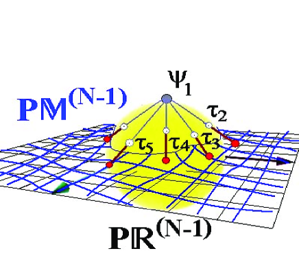
Figure 1: Schematic representation of a projective action of the inverse Laplace operator, ${L}^{-1}:S_{1}^{N-1}-\left\{\psi_{1}\right\}\to P\mathbb{M}^{N-1}$.

Although the Laplace operator $L$ has a trivial eigenvalue $\lambda_{1}=1-\mu_{1}=0$ and therefore is not invertible over $S_{1}^{N-1}$, it is invertible over $S_{1}^{N-1}-\left\{\psi_{1}\right\}$, the orthogonal complement of the first eigenvector $\psi_{1}$ (belonging to the largest eigenvalue of (7) $\mu_{1}=1$) that corresponds to the transient process of random walks toward the stationary distribution $\pi$. The orthogonal complement is homeomorphic to the projective hyper-plane $P\mathbb{R}_{\pi}^{(N-1)}$ constructed by linearly mapping points of the unit hyper-sphere $S_{1}^{N-1}$ from $\psi_{1}$ as the center of projection. The inverse Laplace operator defined by the kernel

$${L}^{-1}\,=\,\sum_{k=2}^{N}\frac{\,\,\mathcal{P}_{k}\,\,}{\,\,1-\mu_{k}\,\,},$$ (23)

in which $\mathcal{P}_{k}$ is the projector (12), is itself a projection operator ${L}^{-1}:S_{1}^{N-1}-\left\{\psi_{1}\right\}\to P\mathbb{M}^{N-1}$ where the $k^{\mathrm{th}}$ coordinate of the projective manifold $P\mathbb{M}^{N-1}$ is subjected to the dilatation $\tau_{k}=\left(1-\mu_{k}\right)^{-1}$, $k=2,\ldots,N$ (see Fig. 1). The kernel (23) defines the Green function (or the Fredholm kernel) describing long-range interactions between eigenmodes of the diffusion process induced by the graph structure.

The convolution with Green’s function gives solutions to inhomogeneous Laplace equations. It is remarkable that such a convolution with the projection operator $\mathbb{P}_{ij}$ gives for the first hitting time the expression

$$t_{ij}\,=\,\sum_{k=2}^{N}\,\frac{\,\,\psi^{\prime}_{ki}{}^{2}-\psi^{\prime}_{ki}\psi^{\prime}_{kj}\,\,}{\,\,1-\mu_{k}\,\,},$$ (24)

which coincides with the result of [16].

It is well known [17, 16] that the matrix of first hitting times $t_{ij}$ is not symmetric, even for a regular graph, and therefore in general $D(i,j)\neq D(j,i)$. However, one can consider its symmetrized analog,

$$d(i,j)\,=\,D(i,j)+D(j,i)\,=\,\sum_{k=2}^{N}\,\frac{\,\,\psi^{\prime}_{ki}{}^{2}-\psi^{\prime}_{kj}{}^{2}\,\,}{\,\,1-\mu_{k}\,\,},$$ (25)

known as commute time [16], the expected number of steps required for a random walker starting at $i$ to visit $j$ for the first time and then to return back to $i$ for the first time. It is easy to check that commute time defined by (25) satisfies all distance axioms.

4.5 The Gram matrix of graph nodes

Each vertex $i\in V$ of the graph $G$ has an image in $P\mathbb{M}^{N-1}$ determined by the vector

$${\bf v}_{i}\,=\,\left(\frac{\,\,\psi^{\prime}_{2,i}\,\,}{\,\,\sqrt{\left(1-\mu_{2}\right)}\,\,},\ldots,\frac{\,\,\psi^{\prime}_{N,i}\,\,}{\,\,\sqrt{\left(1-\mu_{N}\right)}\,\,}\right).$$ (26)

The Gram matrix defined on the set of all vectors $\left\{{\bf v}_{i}\right\}$, $i\in V$, is given by

$$\mathcal{G}_{ij}\,=\,\sum_{k=2}^{N}\,\frac{\,\,\psi^{\prime}_{k,i}\psi^{\prime}_{k,j}\,\,}{\,\,\left(1-\mu_{k}\right)\,\,}.$$ (27)

The diagonal elements $\mathcal{G}_{ii}$ are the first-passage times [16], the expected numbers of steps required for random walkers to reach the node $i$ for the first time starting from any node $l\in V$ randomly chosen among all nodes of the graph $G$ with probability $\pi_{l}$. The elements $\mathcal{G}_{ij}$, $i\neq j$, estimate the expected overlap of random walks towards the nodes $i$ and $j$ starting from a node $l\in V$ randomly chosen among all nodes of the graph $G$ with probability $\pi_{l}$.

Discovering important nodes and quantifying differences between them in a graph is not easy, since the graph, in general, does not possess the structure of Euclidean space. The first passage time, $\mathcal{G}_{ii}$, can be directly used in order to characterize the level of accessibility of the node $i$ in the graph $G$. Various properties of first-passage times have been recently studied in concern with the traffic flow forecasting [21], in order to model the wireless terminal movements in a cellular wireless network [22], in a statistical test for the presence of a random walk component in the repeat sales price models in house prices [23], in the growth modelling of urban agglomerations [24], and in many other works where random walks have been considered directly on city plans and physical landscapes.

In contrast to all previous studies, in our approach, we use first-passage times of discrete time random walks in order to investigate the configuration of urban places represented by means of the spatial graph.

5 Linear automorphisms of urban environments. A case of study

5.1 Spectra of cities

If we take many, many random numbers from an interval of all real numbers symmetric with respect to a unit and calculate the sample mean in each case, then the distribution of these sample means will be approximately normal in shape and centered at 1 provided the size of samples was large. The probability density function of a normal distribution forms a symmetrical bell-shaped curve highest at the mean value indicating that in a random selection of the numbers around the mean (1) have a higher probability of being selected than those far away from the mean. Maximizing information entropy among all distributions with known mean and variance, the normal distribution arises in many areas of statistics.

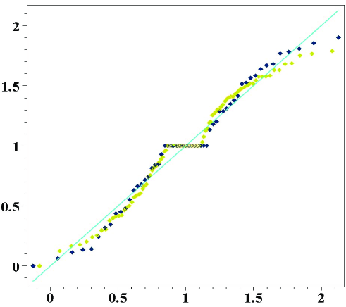
Figure 2: The probability-probability plot of the normal distribution (on the horizontal axis) against the empirical distribution of eigenvalues in the spectra of the city canal networks in Venice and Amsterdam. The diagonal line $y=x$ is set for a reference.

It is interesting to compare the empirical distributions of eigenvalues of the normalized Laplace operator (21) defined on the spatial graphs of compact urban patterns – the spectra of cities – with the normal distribution centered at 1. In Fig. 2, we have shown a probability-probability plot of the normal distribution (on the horizontal axis) against the empirical distribution of eigenvalues in the city spectra (the normal plot) of the city canal networks in Venice (96 canals) and Amsterdam (57 canals). A random sample of the normal distribution, having size equal to the number of eigenvalues in the spectrum has been be generated, sorted ascendingly, and plotted against the response of the empirical distribution of city eigenvalues. The spectra of canal maintained in the compact urban patterns of Venice and Amsterdam look also amazingly alike and are obviously tied to the normal distribution, although these canals had been founded in in the dissimilar geographical regions and for the different purposes. While the Venetian canals mostly serve the function of transportation routs between the distinct districts of the gradually growing naval capital of the Mediterranean region, the concentric web of Amsterdam gratchen had been built in order to defend the city.

It is remarkable that the spectral density distributions shown in Fig. 2 are dramatically dissimilar to those reported for the random graphs of Erdös and Rényi studied by [25, 26]. The classical Wigner semicircle distribution arises as the limiting distribution of eigenvalues of many random symmetric matrices as the size of the matrix approaches infinity, [27]. The eigenvalues of the normalized Laplace operator in a random scale-free graph also follow the semicircle law [28]. City spectra reveal the profound structural dissimilarity between urban networks and networks of other types studied before.

5.2 First-passage times to ghettos

The phenomenon of clustering of minorities, especially that of newly arrived immigrants, is well documented [29] (the reference appears in [30]). Clustering is considering to be beneficial for mutual support and for the sustenance of cultural and religious activities. At the same time, clustering and the subsequent physical segregation of minority groups would cause their economic marginalization. The spatial analysis of the immigrant quarters [30] and the study of London’s changes over 100 years [31] shows that they were significantly more segregated from the neighboring areas, in particular, the number of street turning away from the quarters to the city centers were found to be less than in the other inner-city areas being usually socially barricaded by railways, canals and industries. It has been suggested [32] that space structure and its impact on movement are critical to the link between the built environment and its social functioning. Spatial structures creating a local situation in which there is no relation between movements inside the spatial pattern and outside it and the lack of natural space occupancy become associated with the social misuse of the structurally abandoned spaces.

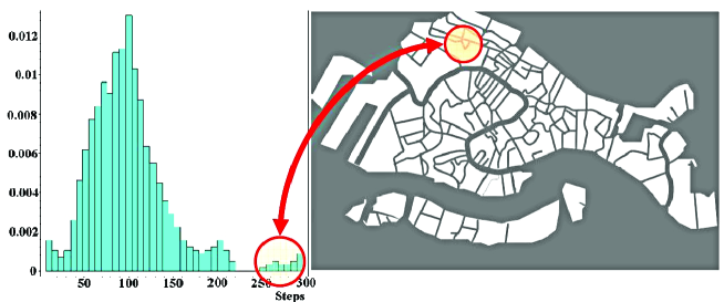
Figure 3: The Venetian Ghetto jumped out as by far the most isolated, despite being apparently well connected to the rest of the city.

We have analyzed the first-passage times to individual canals in the spatial graph of the canal network in Venice. The distribution of numbers of canals over the range of the first–passage time values is represented by a histogram shown in Fig. 3.left. The height of each bar in the histogram is proportional to the number of canals in the canal network of Venice for which the first–passage times fall into the disjoint intervals (known as bins). Not surprisingly, the Grand Canal, the giant Giudecca Canal and the Venetian lagoon are the most connected. In contrast, the Venetian Ghetto (see Fig. 3.right) – jumped out as by far the most isolated, despite being apparently well connected to the rest of the city – on average, it took 300 random steps to reach, far more than the average of 100 steps for other places in Venice.

The Ghetto was created in March 1516 to separate Jews from the Christian majority of Venice. It persisted until 1797, when Napoleon conquered the city and demolished the Ghetto’s gates. Now it is abandoned.

5.3 Random walks estimate land value in Manhattan

The notion of isolation acquires the statistical interpretation by means of random walks. The first-passage times in the city vary strongly from location to location. Those places characterized by the shortest first-passage times are easy to reach while very many random steps would be required in order to get into a statistically isolated site.

Being a global characteristic of a node in the graph, the first-passage time assigns absolute scores to all nodes based on the probability of paths they provide for random walkers. The first-passage time can therefore be considered as a natural statistical centrality measure of the vertex within the graph, [20].

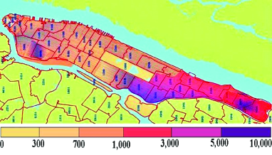
Figure 4: Isolation map of Manhattan. Isolation is measured by first-passage times to the places. Darker color corresponds to longer first-passage times.

A visual pattern displayed on Fig. 4 represents the pattern of structural isolation (quantified by the first-passage times) in Manhattan (darker color corresponds to longer first-passage times). It is interesting to note that the spatial distribution of isolation in the urban pattern of Manhattan (Fig. 4) shows a qualitative agreement with the map of the tax assessment value of the land in Manhattan reported by B. Rankin (2006) in the framework of the RADICAL CARTOGRAPHY project being practically a negative image of that.

Recently, we have discussed in [20] that distributions of various social variables (such as the mean household income and prison expenditures in different zip code areas) may demonstrate the striking spatial patterns which can be analyzed by means of random walks. In the present work, we analyze the spatial distribution of the tax assessment rate (TAR) in Manhattan.

The assessment tax relies upon a special enhancement made up of the land or site value and differs from the market value estimating a relative wealth of the place within the city commonly refereed to as the ’unearned’ increment of land use, [33]. The rate of appreciation in value of land is affected by a variety of conditions, for example it may depend upon other property in the same locality, will be due to a legitimate demand for a site, and for occupancy and height of a building upon it.

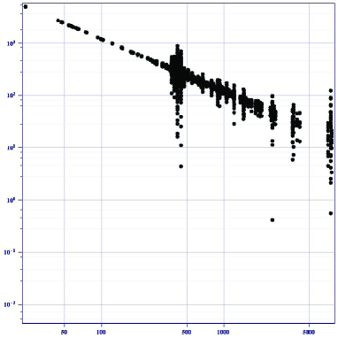
Figure 5: Tax assessment rate (TAR) of places in Manhattan ($/fit²) is shown in the logarithmic scale vs. the first–passage times (FPT) to them.

The current tax assessment system enacted in 1981 in the city of New York classifies all real estate parcels into four classes subjected to the different tax rates set by the legislature: (i) primarily residential condominiums; (ii) other residential property; (iii) real estate of utility corporations and special franchise properties; (iv) all other properties, such as stores, warehouses, hotels, etc. However, the scarcity of physical space in the compact urban pattern on the island of Manhattan will naturally set some increase of value on all desirably located land as being a restricted commodity. Furthermore, regulatory constrains on housing supply exerted on housing prices by the state and the city in the form of ’zoning taxes’ are responsible for converting the property tax system in a complicated mess of interlocking influences and for much of the high cost of housing in Manhattan, [34].

Being intrigued with the likeness of the tax assessment map and the map of isolation in Manhattan, we have mapped the TAR figures publicly available through the Office of the Surveyor at the Manhattan Business Center onto the data on first-passage times to the corresponding places. The resulting plot is shown in Fig. 5, in the logarithmic scale. The data presented in Fig. 5 positively relates the geographic accessibility of places in Manhattan with their ’unearned increments’ estimated by means of the increasing burden of taxation. The inverse linear pattern dominating the data is best fitted by the simple hyperbolic relation between the tax assessment rate (TAR) and the value of first–passage time (FPT),

$$\mathrm{TAR}\,\propto\,\frac{c}{\,\,\mathrm{FPT}\,\,},$$ (28)

in which $c\simeq 120,000\,\,\$\times\mathrm{Step}/\mathrm{fit}^{2}$ is a fitting constant.

References

References

- [1] Population Division of the Department of Economic and Social Affairs of the United Nations Secretariat. 2007. World Population Prospects: The 2006 Revision. Dataset on CD-ROM. New York: United Nations.
- [2] US Bureau of Census Data of Urbanized Areas at http://www.sprawlcity.org/.
- [3] European Environment Agency report Urban sprawl in Europe. The ignored challenge, ISBN 92-9167-887-2 (2006).
- [4] M. Ravallion, ”Urban Poverty.” Finance and Development 44 (3) (2007).
- [5] Hillier, B., Hanson, J., 1984 The Social Logic of Space. Cambridge University Press. ISBN 0-521-36784-0.
- [6] Hillier, B., 1999 Space is the Machine: A Configurational Theory of Architecture. Cambridge University Press. ISBN 0-521-64528-X.
- [7] Hansen, W.G., 1959 Journal of the American Institute of Planners 25, 73-76.
- [8] Wilson, A.G., 1970 Entropy in Urban and Regional Modelling, Pion Press, London.
- [9] Batty, M., 2004 A New Theory of Space Syntax, UCL Centre For Advanced Spatial Analysis Publications, CASA Working Paper 75.
- [10] Penn, A., 2001 Space Syntax and Spatial Cognition. Or, why the axial line? In: Peponis, J. and Wineman, J. and Bafna, S., (eds). Proc. of the Space Syntax International Symposium, Georgia Institute of Technology, Atlanta, May 7-11 2001.
- [11] Jiang, B. Claramunt, C., 2004 Topological analysis of urban street networks. Environment and Planning B: Planning and Design 31, Pion Ltd., 151- 162.
- [12] Volchenkov, D. Blanchard, Ph. 2007 Random walks along the streets and canals in compact cities: Spectral analysis, dynamical modularity, information, and statistical mechanics. Physical Review E 75(2), id 026104.
- [13] Volchenkov, D., Blanchard, Ph. 2008 Scaling and Universality in City Space Syntax: between Zipf and Matthew. Physica A 387/10 pp. 2353-2364. doi:10.1016/j.physa.2007.11.049.
- [14] A. Chan & C. Godsil. Symmetry and Eigenvectors. In Graph Symmetry, Algebraic Methods and Applications, edited by G. Hahn & G. Sabidussi, pp. 75 106. Dordrecht, The Netherlands: Kluwer, (1997)
- [15] Ph. Blanchard, D. Volchenkov, ”Intelligibility and first passage times in complex urban networks”, Proc. R. Soc. A 464, 2153-2167; doi:10.1098/rspa.2007.0329 (2008).
- [16] Lovász, L. 1993 Random Walks On Graphs: A Survey. Bolyai Society Mathematical Studies 2: Combinatorics, Paul Erdös is Eighty, Keszthely (Hungary), p. 1-46.
- [17] Aldous,D.J., Fill, J.A. Reversible Markov Chains and Random Walks on Graphs. A book in preparation, available at www.stat.berkeley.edu/aldous/book.html.
- [18] Horn, R.A., Johnson, C.R., 1990 Matrix Analysis(chapter 8), Cambridge University Press.
- [19] Chung, F. 1997 Lecture notes on spectral graph theory, AMS Publications Providence.
- [20] Blanchard, Ph., Volchenkov, D. ”Mathematical Analysis of Urban Spatial Networks”, in Series: Understanding Complex Systems XIV, ISBN: 978-3-540-87828-5, Springer (2008).
- [21] S. Sun, Ch. Zhang, Yi. Zhang, ” Traffic Flow Forecasting Using a Spatio-temporal Bayesian Network Predictor”, a chapter in Artificial Neural Networks: Formal Models and Their Applications, pp. 273-278, Book Series Lecture Notes in Computer Science, Vol. 3697/2005, Springer (2005).
- [22] B. Jabbari, Zh. Yong, F. Hillier, ”Simple random walk models for wireless terminal movements”, Vehicular Technology Conf., 1999 IEEE 49th Vol. 3, pp.1784 - 1788 (Jul 1999).
- [23] R.C. Hill, C.F. Sirmans, J.R. Knight, Regional Science and Urban Economics 29 (1), 89-103(15) (1999).
- [24] M. Pica Ciamarra, A. Coniglio, ”Random walk, cluster growth, and the morphology of urban conglomerations”. Physica A 363 (2), pp. 551-557 (2006).
- [25] I.J. Farkas, I. Derényi, A.-L. Barabási, T. Vicsek, ”Spectra of “Real-World” graphs: Beyond the semi-circle law.” Phys. Rev. E 64, 026704 (2001).
- [26] I. Farkas, I. Derényi, H. Jeong, Z. Neda, Z.N. Oltvai, E. Ravasz, A. Schubert, A.-L. Barabási, T. Vicsek, ”Networks in life: Scaling properties and eigenvalue spectra ”. Physica A 314, 25 (2002).
- [27] Ya. G. Sinai, A. B. Soshnikov, Functional Analysis and Its Applications 32 (2), 114-131 (1998).
- [28] F. Chung, L. Lu, V. Vu, ”Spectra of random graphs with given expected degrees.” Proc. Natl. Acad. Sci. USA. 100(11): 6313-6318. (2003); Published online doi: 10.1073/pnas.0937490100.
- [29] L. Wirth, The Ghetto (edition 1988) Studies in Ethnicity, transaction Publishers, New Brunswick (USA), London (UK) (1928).
- [30] L. Vaughan, World Architecture, 185, pp. 88-96 (2005).
- [31] L. Vaughan, D. Chatford & O. Sahbaz Space and Exclusion: The Relationship between physical segregation. economic marginalization and povetry in the city, Paper presented to Fifth Intern. Space Syntax Symposium, Delft, Holland (2005).
- [32] B. Hillier, The common language of space: a way of looking at the social, economic and environmental functioning of cities on a common basis, Bartlett School of Graduate Studies, London (2004).
- [33] Bolton, R.P., Building For Profit, Publisher: Reginald Pelham Bolton (1922).
- [34] Glaeser, E.L., Gyourko, J., Why is Manhattan So Expensive?, Manhattan Institute for Policy Research, Civic Report, No. 39 November 2003.